Recovery of Low-Grade Heat (Heat Waste) from a Cogeneration Unit for Woodchips Drying: Energy and Economic Analyses


1
Institut des Sciences des Matériaux de Mulhouse IS2M-UMR 7361CNRS-UHA, 3 bis rue A, Werner, 68098 Mulhouse CEDEX, France
2
Réseaux de Chaleur Urbain d’Alsace (RCUA) 17 Place des Halles, 67000 Strasbourg, France
*
Author to whom correspondence should be addressed.
Energies 2019, 12(3), 501; https://doi.org/10.3390/en12030501
Submission received: 19 December 2018
/
Revised: 30 January 2019
/
Accepted: 31 January 2019
/
Published: 5 February 2019
(This article belongs to the Special Issue The 6th International Conference on Sustainable Solid Waste Management: NAXOS 2018)
Abstract
:The aim of this paper is to improve the operating share of a biomass cogeneration unit by using unavoidable heat waste heat recovered from a district network heating used for drying woody biomass’ return water (law-grade temperature heat). The optimal operating conditions of a drying unit added to the system were estimated from an energy and a financial point of view, applying four objective functions (drying time, energy consumption, energy balance, and financial performance of the cogeneration unit). An experimental design methodology used heat for the implementation of these functions and to obtain an operating chart. Numerical modelling was performed to develop a simulation tool able to illustrate the unsteady operations able to take into account the available waste heat. Surprisingly, the model shows that the right strategy to increase the financial gain is to produce more warm water than necessary and to consequently dispose higher quantities of unavoidable heat in the network’s return water, which heat up the drying air at a higher temperature. This result contrasts with the current approaches of setting-up cogeneration units that are based on the minimization of the heat production.
1. Introduction
1.1. General Introduction
In the current global context, energy management and energy saving technologies are of strategic importance in the transition to a more efficient, sustainable, and low carbon energy system. Indeed, the world energy consumption and demand is rapidly rising [1] and the development of alternative and more sustainable energy sources have become a priority in order to decrease environmental issues. Unfortunately, certain scenarios predict that renewable energies will not be sufficient to meet overall energy needs [2]. One of the most promising solutions is to reduce heat waste when using alternative energies. Heat waste represents a significant fraction of the total energy consumption, but the variable geographical location, process source, amount, quality, and availability issues make energy recovery and utilization challenging. Gingerich et al. [3] investigated the full potential, quality, and possible use of waste heat coming from thermal power generation units in the US. Heat waste streams were analyzed differently in terms of temperature, seasonal availability, and amount, and consequently, the identified applications were disparate [4].
Many studies have been devoted to the use of extra heat or heat waste coming from industrial units in district heating [5]. The transformation into power or electricity by Organic Rankine Cycles (ORC) was also investigated [6,7]. However, a dramatic lack in studies concerning the recovery of low-grade heat (T < 70 °C) has been identified in the recent literature. This fraction of waste energy at low temperatures is commonly defined as “unavoidable waste heat”.
Highly efficient cogeneration units produce electricity, heat, and hot water for domestic, municipal (district heating) and industrial issues. The hot water produced is then distributed to the downstream users in the pipeline of a heating network. After use, the return water must be cooled down before being re-injected in the heat system of the steam generator. For this reason, the heating network is generally equipped of cooling towers to dissipate the residual heat from the return water. This low-grade heat (temperature in the 30–60 °C range) called “unavoidable waste heat” is completely lost in this process [8]. Besides, the cooling system needs extra-energy for operating valves, pumps, and extra-costs to supply the chemical products for antibacterial water treatments.
In France, the resale grid-connected tariff of power is directly proportional to the cogeneration plant efficiency (ratio between the usable energy and the nominal fuel power) [9]. The recovery of “unavoidable waste heat” appears then to be very interesting from environmental, energetic, and financial points of view because [10]: (i) the global plant efficiency increases; (ii) the resale tariff of electric power, and thus, the profit of the industrial plant increases; (iii) the use of extra energy and water treatment products in the cooling towers is minimized or even eliminated; (iv) the waste heat is not dissipated in the atmosphere.
1.2. Low-Grade Heat Recovery (T < 70 °C)
A current challenge is to identify new market applications for this energy [11,12]. Indeed, the efficient use of heat at low temperatures is limited to a few applications such as power generation from ORC [13,14], which has poor efficiency at low temperatures, heating of horticultural greenhouses [12], preheating steps in industrial processes [15,16], and heat supply for anaerobic digestion of biomass [17]. Due to the geographical location of the power units (i.e., generally close to residential buildings and municipal infrastructures, integrated to district heating networks), it is seldom possible to develop such “unavoidable” heat waste recovery systems. Several studies have a major aim to evaluate the potential of process sites for low-grade heat recovery, especially the efficiency of various options (e.g., ORC, Kalina cycles, adsorption heat pumps, chillers, etc.) [18]. The optimization of cogeneration systems was also numerically studied [19]. Other works focused on specific techniques to recover heat waste. For example, the use of heat pumps operating in various production sites [20] or the implementation of chemisorption-based energy storage systems [21]. As the domestic demand of heat fluctuates as a function of the weather, the temperature of the return flow, and consequently the availability of heat waste in the heating network, will be variable [22]. One possible alternative way to use this low-grade heat is by pre-drying or drying wet materials, such as fuel pre-drying [16,23], sewage sludge drying (including heat from the biochemical process treatment [24]), and biomass drying for energy purposes [17,25,26,27]. Indeed, woody biomass coming from forestry contains up to 50% in water weight and its combustion is consequently energetically unattractive. By eliminating around 20% of the initial water, the heat capacity increases from 2.2 to 3.9 kWh·kg−1. In this way, the dried biomass can be stored (if protected to avoid further moisture absorption) and used as fuel with higher heat capacity [28].
1.3. Industrial Setup
The former industrial installation consisted in a biomass cogeneration unit (17.2 MW) producing electricity (5.2 MW) and hot water (12 MW), which was used to distribute the heat in a district heating network.
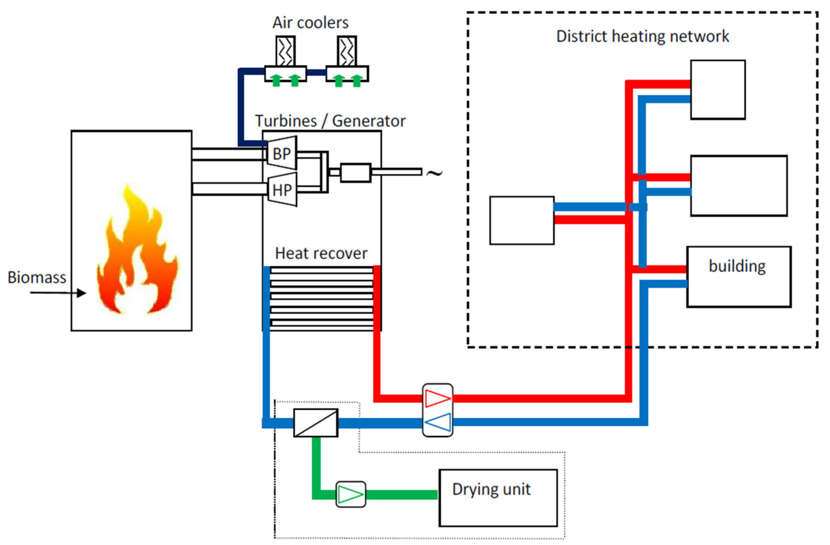
Figure 1 shows a schematic diagram of the cogeneration unit. The biomass used (woodchips, corncob, or wood wastes) was moved by a conveyer belt from the tank and introduced by a feeder screw in the boiler (fluidized bed). Electric power was produced from two coaxial turbines (HP backpressure turbine and BP turbine). The second (0.1 bar, 45 °C) could not be engaged as it operates only in the low season, where it is cooled by a water loop coming from air coolers. The district heating network was 10 km in length and covered heat needs of 3500 housing equivalents. Before the installation of the drying set-up (dotted box in Figure 1), the return water (law-grade temperature water) was re-injected into the boiler. After modifications (installation of the drying system), the return water was directly used to heat up the drying air in a heat exchanger. The annual electricity production was about 25 GWh and the useful heat output was 40 GWh.
1.4. Methodology
The main objective of this work was to determine and optimize the process parameters to dry biomass using “unavoidable energies”. A three-pronged approach (biomass characterization, experimental study, and numerical treatment of results) was used to investigate the drying efficiency as a function of time, available energy, and financial gain. The industrial interest of such work is to identify the best operating conditions for both companies: the heat and electricity producer and the wood supplier. This study provides a global approach, where the interactions between the two industrial activities are taken into account in the numerical modeling.
At the laboratory scale, an experimental study was carried out on a pilot dryer (scaled-down reproduction of the industrial installation) and a numerical tool was developed to simulate the dryer performances. From these experimental and simulated results, relevant operating information were obtained, allowing us to construct the operating chart. Indeed, several studies investigated the optimization of wood drying processes in the past [29,30]. They concluded that the optimization of drying operations is a difficult combinatorial problem and that the calculation of a complex objective function including criteria (e.g., economical, technical, performance, time, etc.) requires a modeling approach and various assumptions.
2. Materials and Methods
2.1. Experimental Setup
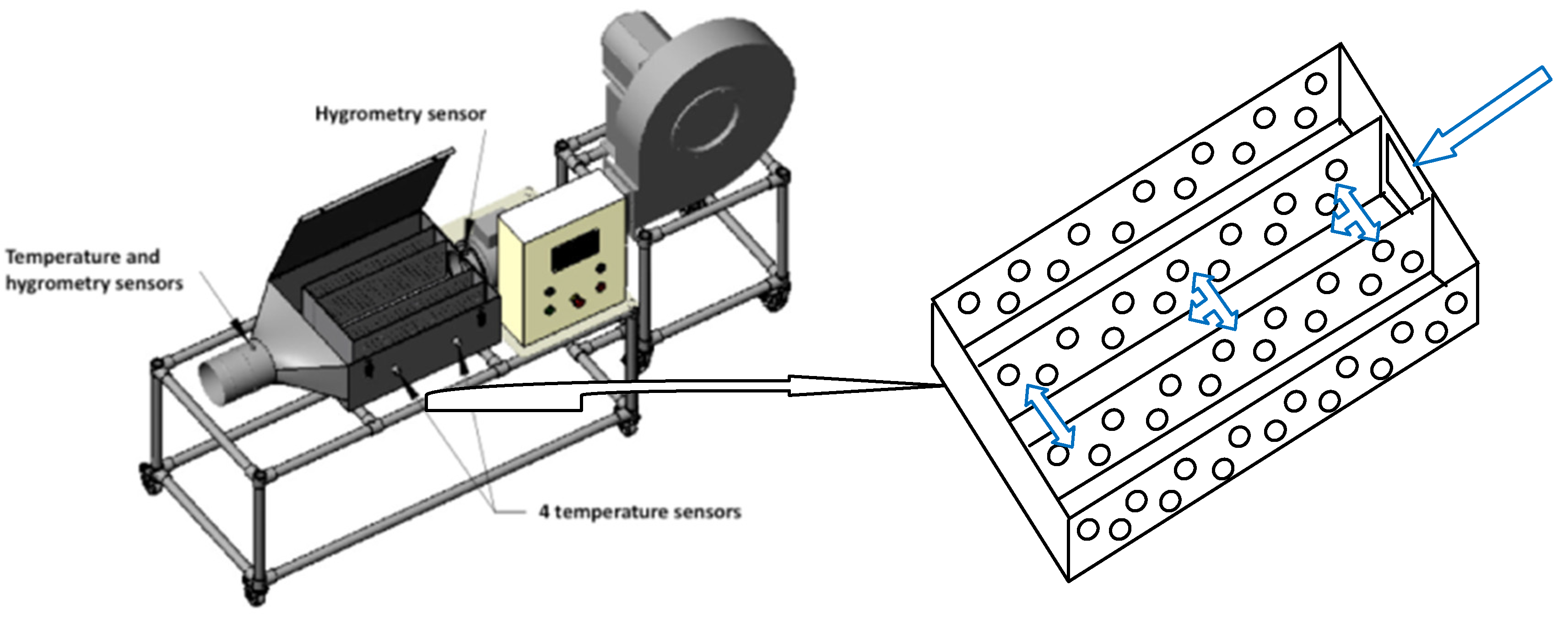
The experimental equipment is the pilot dryer (T.I.A., Bollène, France) represented in Figure 2.
The pilot dryer [31] consisted of a small-scale reproduction (1/10th scale model) of the industrial dryer (Réseaux de Chaleur Urbains d’Alsace company). The ambient air was drawn by a fan, heated by electrical heaters, and then introduced in the drying chamber. Air velocity, temperature, and humidity WERE directly measured USING sensors connected to a control panel. The biomass was then placed into the drying chamber, in which it was composed of two parallel beds. The drying chamber, containing the biomass, was then placed on a balance, able to continuously measure the mass loss, and indirectly the humidity content. Four supplementary thermocouples allowed for temperature measurement inside the biomass beds. Further, one thermocouple and a sensor were placed at the exit of the dryer to measure the temperature and humidity of the exhaust air. All experimental data were recorded in real time with a data acquisition system integrated into the control panel.
The physico-chemical properties of the different wood biomasses were measured (i.e., density, specific heat, and thermal conductivity) at different temperatures and water contents. The same properties were also determined for each material in the configuration used during drying (bed of biomass chips), thus taking into account the presence of air between the wood chips.
2.2. Biomass Thermo-Physical Properties
The selected biomasses were wood chips from forestry. The length and width of the chips were in the 1–5 cm range, while the thickness was lower than 2.5 cm. The initial water content was in the 40 to 50 mass% (wet basis) range.
To correctly simulate the biomass drying, the thermo-physical properties of the biomass, as a function of water content and temperature, have to be integrated into the model. The properties of the biomass bed are required, too. For this reason, the density of the wood was obtained by mass balance. A weighed mass of chips was introduced in a vessel of known volume and the empty space between the chips filled with sand. The apparent density of the biomass bed was then directly obtained by weighting the chips/sand mixture.
The water content was measured using the weight difference of the wood samples before and after drying (at 105 °C during 24 h).
The specific heat of the wood was obtained by calorimetric analysis performed in an adiabatic calorimeter, while the thermal conductivity of the biomass beds was estimated by using a guarded hot plate apparatus. Such experiments allowed for the measurement, in the steady state, of heat flow passing through the biomass for a given temperature gradient.
2.3. Modelling of the Drying Process
The model used in this study was a classic drying model already accurately detailed in the literature [32,33,34]. Mass and heat transfer were assumed to be monodimensional (x) and time dependent (t) in the biomass bed [35]. Hence, the drying process was described using a set of three coupled and non-linear differential equations (Equations (1)–(3)), representing the water mass balance (Equation (1)) and the energy balances in air (Equation (2)), as well as the biomass (Equation (3)), respectively. An additional equation was used to approximate the drying kinetics (Equation (4)).
The water mass balance in the wood bed was:
The energy balance of air passing through the biomass bed was:
The energy balance in the biomass was:
The boundary conditions were as follows:
The inlet temperature T (x = 0) and humidity of air H (x = 0) are constant. The biomass was assumed to be at room temperature and the biomass water content was equal to M0 before drying.
Kinetic modelling of the drying process:
An empirical equation [36,37] was used to simulate the drying process. This equation, called the Henderson and Pabis equation or the Lewis equation for a = 1, assumed a diffusive control of the drying process. This equation was previously used for various agricultural products (e.g., bagasse, peanuts) and is particularly suitable for wood residues (chips, bark, small branches of softwood).
The biomass humidity (dry basis) at the equilibrium was calculated using the equation developed by Zuritz et al. [38]. For wood, this equation provides reliable results in the 21.1 °C to 71.1 °C range [39].
With the critical temperature of water.
Numerical calculation:
The model consisted of four equations and associated boundary conditions with four unknown factors (H, M, T, and θ). This system was spatially discretized according to the finite difference method and the Euler method, used for time integration. The different thermo-physical properties of air and biomass were calculated as a function of temperature and water content. Simulations were performed according to an explicit scheme, which previously required an adjustment of the discretization parameters.
2.4. Experiments and Results Analysis
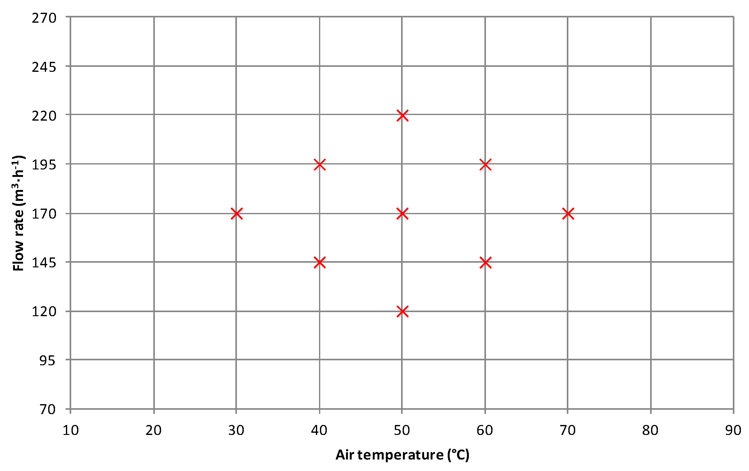
Experiments were performed according to the Design of Experiments (DOE) (central composite design), as shown in Figure 3. This approach allowed us to optimize the utilization of experimental and numerical results [40]. On the basis of the DOE, the studied functions Y can be approximated by the quadratic function of air temperature and flow rate, reported as follows:
The five parameters were numerically estimated by minimizing a quadratic criterion between experimental and calculated values. This methodology required a minimum of nine experimental tests to perform the calculation and some additional tests to estimate the relevance of the results. To compare the five parameters, two operating conditions were normalized in the [−2,2] range. and represented the normalized values of air temperature and flow rate, respectively. This methodology allowed us to estimate the influence of each operating condition on the studied function, as was previously reported in similar studies [41,42,43,44,45].
To estimate the dryer performances and the efficiency of the waste heat recovery process, four response functions were taken into account: (i) the drying time (td): the time to reach the final water content (Mf); (ii) the heat (Q) used to dry biomass from the initial to the final humidity (expressed per kilogram of evaporated water):
(iii) the energy balance (E): the gain in heat value (heat upgrade obtained after drying of the biomass) divided by the heat used to dry, as follows:
where and (J·kg−1) are the final and initial lower heating values, respectively; and (iv) the financial gain (FG): ratio between the gain of the cogeneration unit including the drying process and the gain of the cogeneration unit without the drying process.
and are respectively the feed-in tariffs of electric power and heat. The numerator of FG corresponds to the actual financial gain of the cogeneration system in the presence of the drying unit, while the denominator is the financial gain in absence of the drying unit. This gain is the sum of the benefit obtained by selling electricity (Ugenerated − Uused) at the feed-in tariff (Costelec) and the benefit obtained by selling heat (Qused) at the actual net price of heat per kWh.
The electricity used to run the global system includes the energy consumed from the fan, for the circulation of the drying air (in the numerator) and the energy required from the cooling towers (in the denominator). Recent results obtained during two years of operation shows that the drying unit used 12 thermal GWh (compared to 80 GWh of heat generated) and 0.14 GWh of electric power (compared to 49 GWh of electricity produced).
The difference between the numerator and the denominator corresponds to the feed-in tariff of electric power, which is linearly indexed (case study based on the French tariffs) to the cogeneration efficiency.
Numerical approximation of experimental functions td, E, Q and FG were performed by solving a system of n equations (number of tests) with six unknowns. The six model parameters were estimated by minimizing the sum of square errors with y = E, Q, td, or FG.
The quality of numerical approximation was examined from five statistic values:
- (i)
- the determination coefficient r2;
- (ii)
- the standard error of estimate S = ;
- (iii)
- the Marquard’s percent;
- (iv)
- standard deviation MPSD = ;
- (v)
- the mean absolute error EABS = ;
- (vi)
- the mean relative error RE = .
3. Results
3.1. Experimental Results
Experiments were performed accordingly to the central composite design. The operating conditions in terms of air temperature and air mass flow rate are shown in Figure 3. Table 1 shows the results obtained for the 10 experimental tests in terms of drying time, heat used for drying, energy balance, and financial gain (projection on a real cogeneration installation).
At first, the six experimental tests were performed at the same operating conditions (50 °C and 150 m3/h) to assess the experimental error. One of these tests shows anomalous results probably due to a weak initial moisture. The drying time obtained for the five remaining tests are 1.7 h ± 0.12 h (standard deviation = 0.07).
The pertinence of the quadratic approximations of the four studied functions is investigated for 10 experimental results (9 of the DOE + 1 additional test). The results are presented in Table 2.
The results show that numerical approximation of FG fits well the experimental results and, to a certain extent, the Q and E functions. The worse results are obtained for drying time and are in anyway acceptable.
Starting from these equations, response surface plots were generated for different operating conditions.
3.2. Drying Time
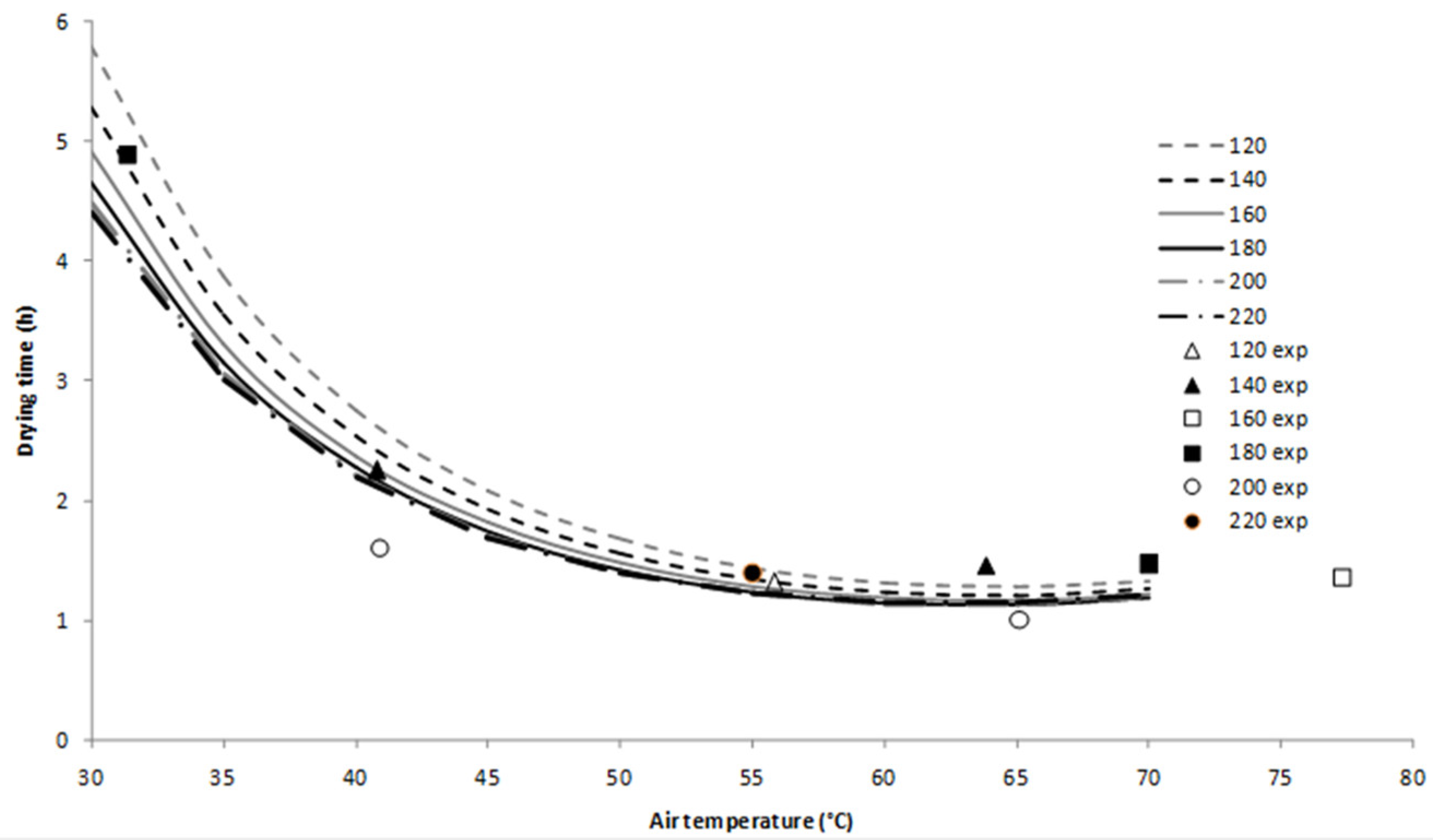
Figure 4 shows the calculated drying time as a function of air temperature and flow rate. The temperature and, at a lower extent, the air flow, which modified the drying performance. When the air temperature was higher than 60 °C, the drying time slightly decreased. Moreover, the influence of the air flow was quite limited in the studied temperature range (40 < T< 80 °C).
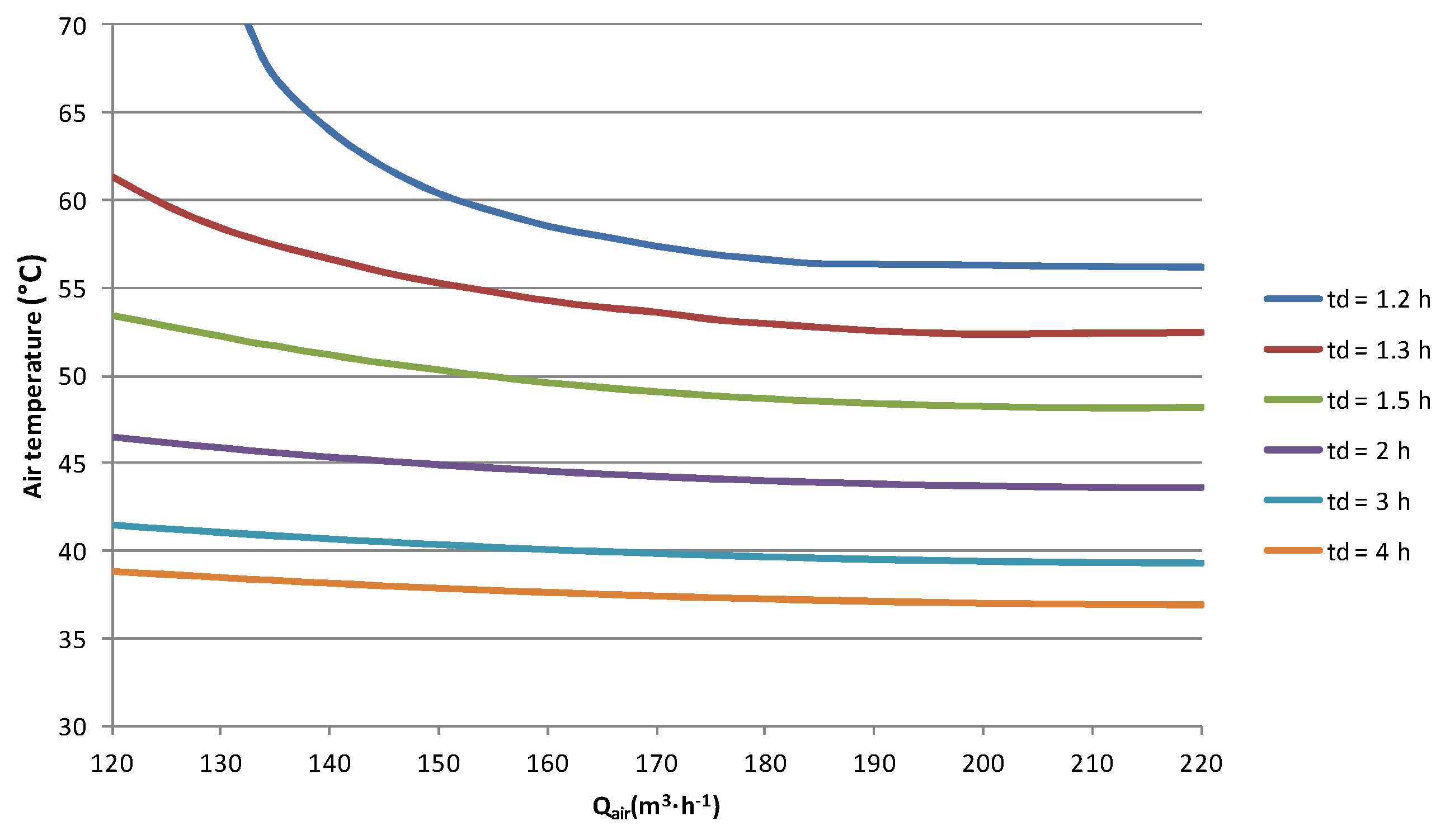
Figure 5 shows the isocontours of the drying time in a diagram, where the air temperature is plotted as a function of the air flow rate (obtained by the DOE equation). To satisfactorily approximate the drying time (minimization of errors between experimental and calculated values), a polynomial equation was applied with the logarithm of the drying time.
As expected, the drying time decreased for high temperatures and flow rates. However, for a mass flow rate higher than 170 m3·h−1, only the drying time displayed a slight variation. Indeed, the effect of flow rate is significant at high temperatures and a low flow rate. Under these conditions, the extraction of water from the material was faster and the air flow rate was the limiting factor in the mass transfer process. Sepulveda et al. [46] reached to the same conclusions for drying of waste from cork industry. These curves were used as an industrial chart for the process optimization.
3.3. Energy Analyses
Figure 6 shows the energy consumption for the wood chips drying process (expressed per kilogram of evaporated water) as a function of the operation conditions (air temperature and flow rate). The numerical approximation of the energy used was performed by studying the square root of Q.
As expected, energy increased with the temperature and, even more significantly, with the flow rate. However, the energy increase was less important in the 30–45 °C temperature range.
The best drying conditions in terms of time (high temperature T > 50 °C and Qair > 170 m3·h−1) corresponded to the highest energy consumption. On the contrary, the lowest energy consumptions were reached for low air flows Qair < 160 m3·h−1 and T < 60 °C. These two functions present opposite behavior. The best (drying time and energy consumption) ratio could be reached at intermediate flow rates (in the 160–170 m3·h−1 range) and intermediate temperatures (between 50 and 60 °C).
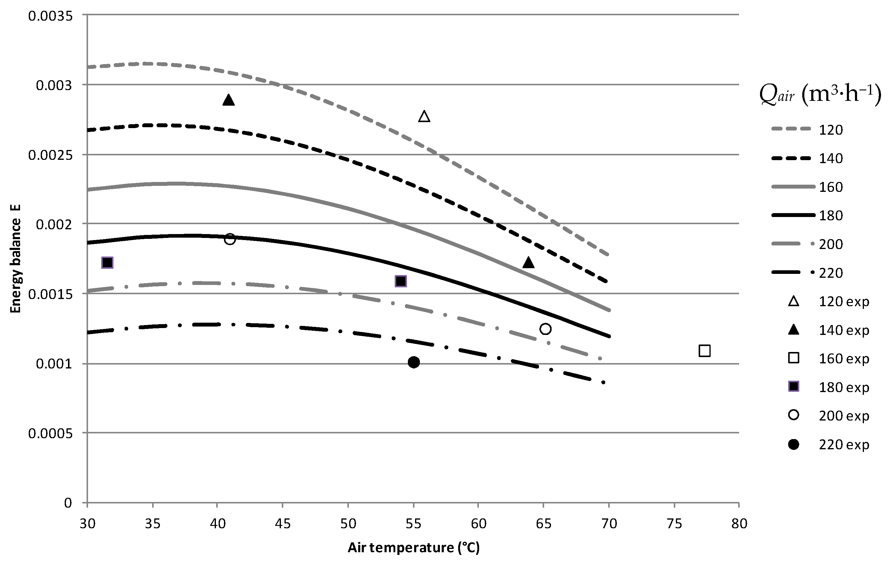
Figure 7 reports the energy balance as a function of air temperature at different operating conditions (various air flow rates). The numerical approximation of the energy balance was carried out by studying the logarithm of E. Taking into account only the energy capacity of biomass combustion, it turned out to be more interesting to dry at a low air temperature and low flow rate. The rapider the drying, the lower the drying efficiency. As previously observed, the optimal conditions of drying, in terms of time (Figure 4, T ≥ 50 °C), energy balance (Figure 6, 30 ≤ T ≤ 55 °C, Q minimal), and energy consumption (Figure 5, 30 ≤ T ≤ 50 °C, Q ≈ 120 m3·h−1), were reached for low air flow rates (i.e., 120–140 m3·h−1) and intermediate temperatures (T ≈ 50 °C).
3.4. Kinetic Results
Table 3 gives the kinetic parameters, as calculated by Equation (4). The graph of versus time, allows for the estimation of k (slope of the linear curve) and a (intercept). First, all the curves are linear with an interception close to 0. In these conditions, the pre-exponential factor can be assumed to be equal to 1.
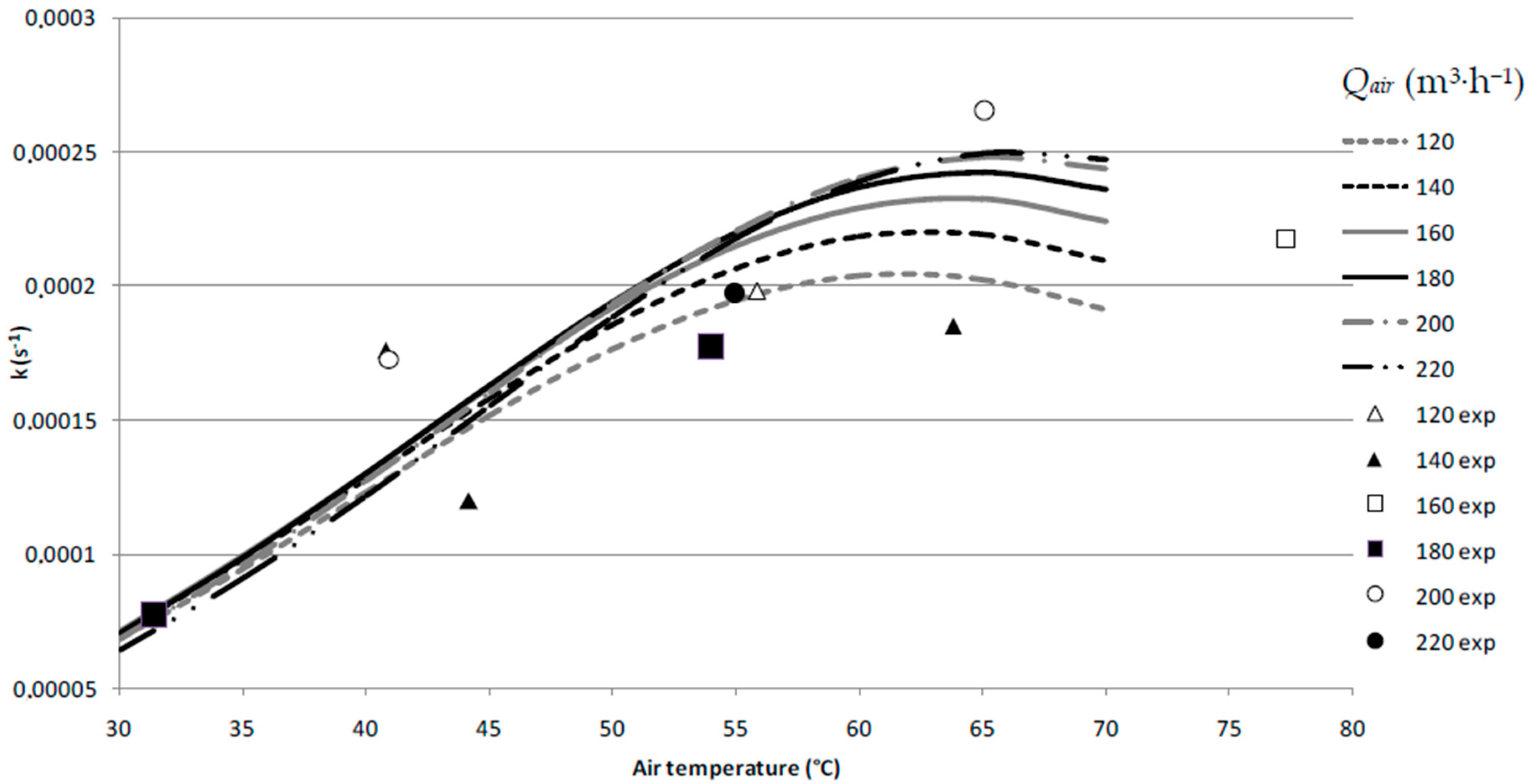
Figure 8 shows the kinetic parameter k estimated from the experimental results for the applied operating conditions (points) and the results from the DOE investigation (lines). The air flow rate seems to have little effect on the kinetic parameter, except at high temperature. This behavior can be attributed to the fact that the limiting factor is the diffusion of water into the material. When the temperature increased, water diffusion was more rapid, and the effect of air flow rate became significant. Contrary to the four previous studied functions, the numerical approximation using the quadratic equation gave uncertain results. Indeed, no clear trend emerged from the experimental results, except an increase of the kinetic parameter with the air temperature.
3.5. Numerical Results
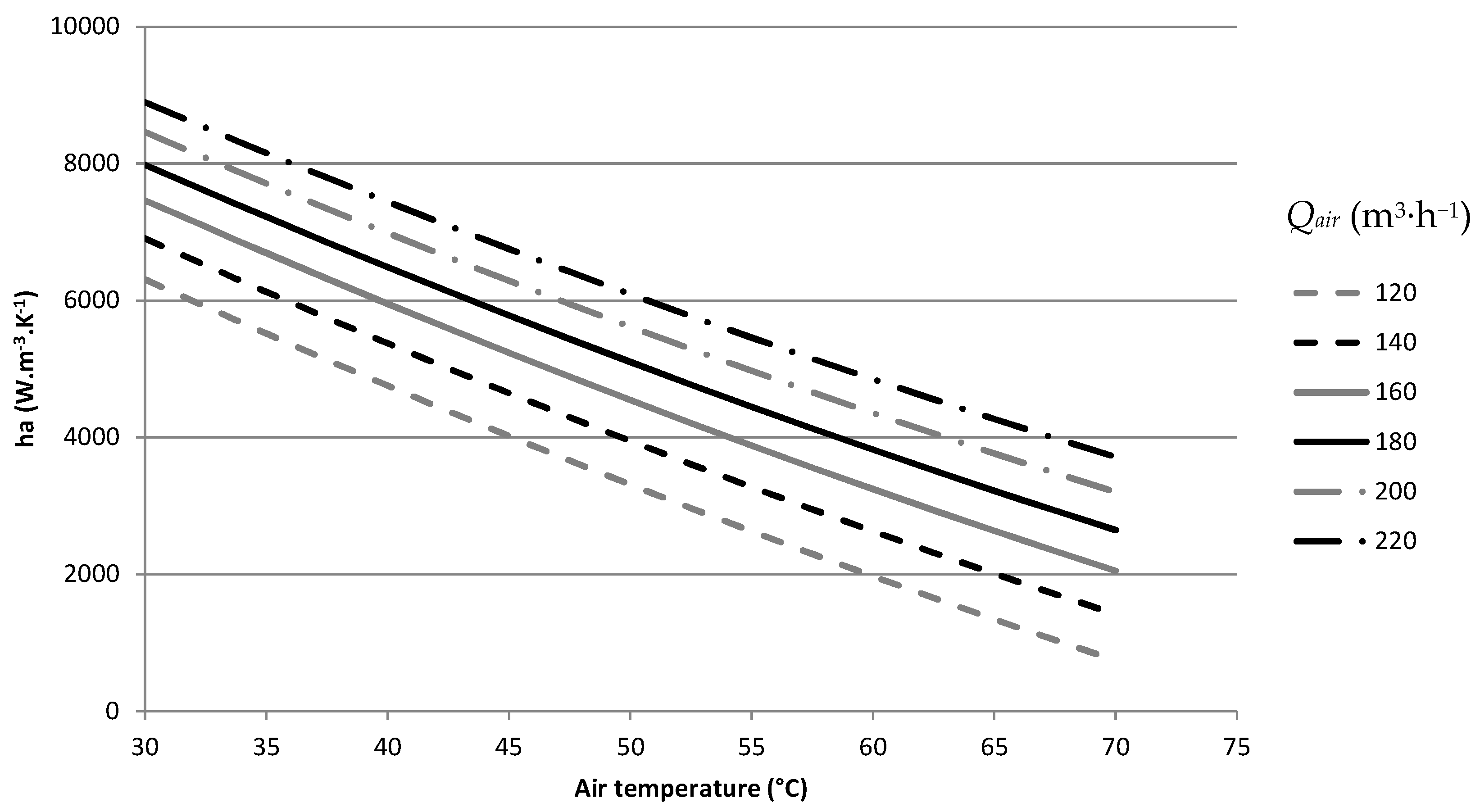
After validation, the numerical tool will be able to perform simulations in different operating conditions. The program calculated temperatures and water content into the biomass as a function of time and biomass bed depth. To approximate and simulate drying experiments, the knowledge model required the estimation of three parameters (the two kinetic parameters and ha, the coefficient of heat transfer between air and biomass). The identification of these three parameters was not simultaneous, because the kinetic parameters were estimated by approximation of the experimental water contents into the material and ha by the temperature profiles in the bed of biomass. The kinetic parameters were almost identical to those directly obtained by plotting the logarithm of the average water content versus time. These results were expected due to the use of exactly the same equation integrated to the model. The only difference was the calculation methodology of the equation: average condition and spatial resolution. Starting from this kinetic estimation, only the volumetric heat transfer coefficient was numerically estimated to approximate the experimental results (temperatures and biomass water contents). The best-fitted convective coefficient is shown in Figure 9, according to the operating conditions.
The coefficient linearly increased with the air mass flow rate and almost linearly decreased with the applied air temperature values. These results are in good agreement with the kinetic theory of gases (ideal gas). Indeed, the coefficient is often calculated using correlations (Nusselt number) in the general form; Nu = C∙Reα∙Prβ with α > β > 0. The Reynolds number (Re) is linearly proportional to the fluid velocity that explains the increase of the coefficient with the air mass flow rate. According to the kinetic theory of gases for an ideal gas, the dependence in temperature of the convective coefficient is .
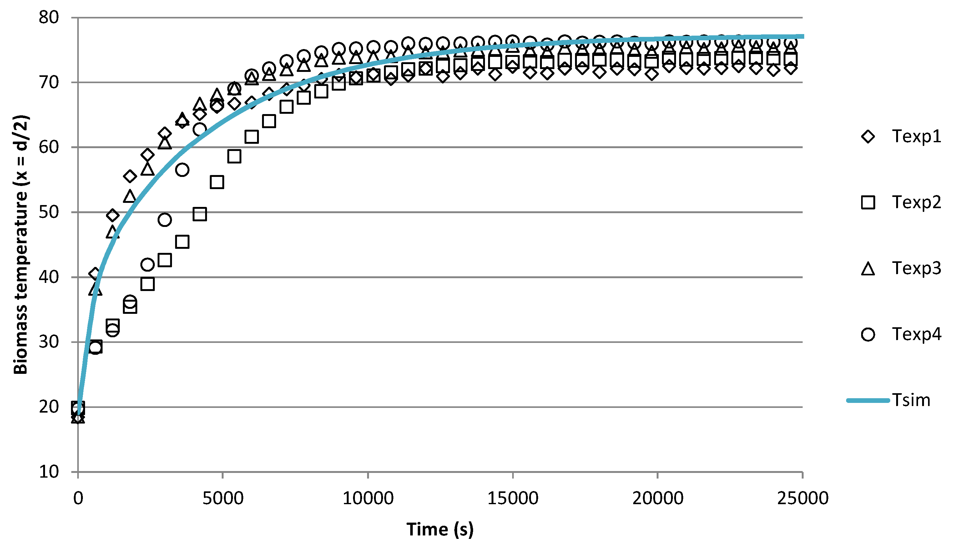
Starting from these equations for kinetic and heat transfer, the program can be used in a predictive way. To evaluate the predictive capacity of the numerical tool, the model was validated by comparing experimental and numerical temperature profiles (in the middle of the biomass bed). Figure 10 and Figure 11 show the calculated temperature profiles compared to the four experimental profiles obtained with the operating conditions of test 5 and test 6, respectively.
The experimental and the numerical results reported in Figure 10 and Figure 11 are in good agreement. The biomass temperature increasing and the equilibrium temperature are well approximated by the numerical model, as well as the evolution of the biomass water content. The numerical approach can simulate the biomass drying process in the studied range of operating conditions and, after a change of scale, the industrial drying process.
4. Influence of Drying Process on the Cogeneration Unit Performances
Economic Analysis
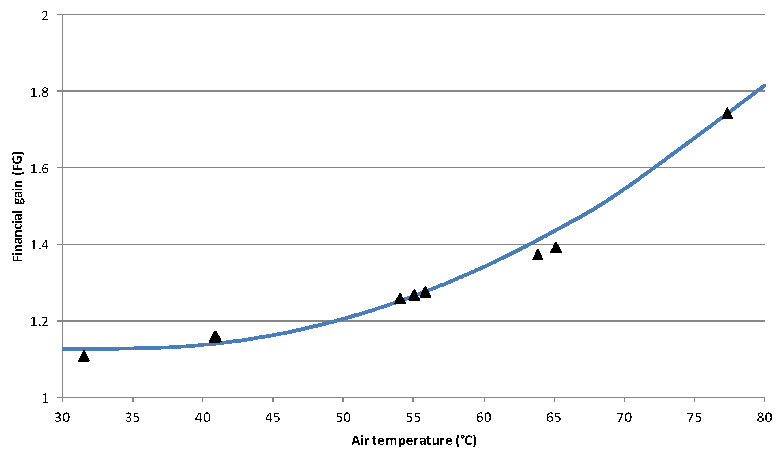
Figure 12 shows the financial gain, which is the ratio between the gains obtained in presence and in absence of the drying process, as a function of air temperature. The calculation is performed with the feed-in tariffs 2017: costheat = 0.05 and costelec = 0.045 + 0.1253 × Rcogen, where Rcogen is the cogeneration efficiency: ratio between energy (heat and electric power) generated and biomass disposal defined as follow:
The experimental results (triangular dots) from the 10 tests are obtained for different mass flow rates and temperatures. The numerical approximation of the financial gain is obtained by the FG function. First of all, the obtained best-fitted parameters show that there is no significant influence of the air flow rate. Thus, the influence of this parameter can be neglected with respect to the air temperature. From this assumption, the financial gain can be approximated by a quadratic equation depending only on the air temperature (r² = 0.982):
This result can be explained by the fact that the energy used to produce the air flow rate (fan) is negligible compared to the heat and electric power generated. Secondly, it can be observed that FG increases with the air temperature. Indeed, the highest financial gain is obtained when the cogeneration efficiency is maximized and so the feed-in tariff of the electric power. This is reached when all the produced heat is sold to the network costumers, and the waste heat is used for drying the biomass. If the biomass drying is carried out by a third party, the heat sold for this purpose increases the cogeneration efficiency. When the demand is lower (i.e., during a particularly warm winter season) the financial gain can be guaranteed by selling the exceeding heat for other purposes. Indeed, the production of more energy than needed (especially for heating purposes) is relevant for the cost effectiveness of the cogeneration unit. This result is very interesting for the future strategy of territory’s development, in particular for planning of eco-neighborhoods. Nowadays, the construction of new housing is designed to obtain the best individual performances (in terms of insulation, power generation, indoor heating, and so forth). However, the current strategy generates problems from a collective point of view, as it creates a mismatch between the heat demand and the amount of energy actually generated and delivered via the heating network. In this context, the integration of a cogeneration unit is a difficult matter due to the need to continuously adjust the power and the heat generation to the heat demand. This functioning mode becomes a financial problem for energy suppliers that are obliged to operate in degraded mode. From these results, it appears that coupling power and heat generation in domestic and collective projects is feasible.
5. Conclusions
A three-pronged approach (experimental, numerical, and DOE methodology) was used to investigate the optimization of a cogeneration unit by using unavoidable energy. This energy was used to dry biomass from the forestry industry. At first, four functions connected to the performances of the dryer and the cogeneration unit were studied, using the DOE methodology approach. As expected, the decrease of the drying time with the air flow rate and temperature was observed. On the other hand, the financial gain results were surprising. The financial gain increased when there was no heat demand, which corresponded to the configuration in which the heat produced was fully used to dry the biomass. This unobvious result was due to the resale grid-connected tariff of power, which was directly proportional to the cogeneration efficiency. Because of the way the overall system operates, the financial gain did not depend on the energy producer (cogeneration unit) alone. Indeed, companies and municipalities use heat via the district heating system (for hot water and heating needs) and other companies need heat to dry biomass. The needs of one are not necessarily consistent with the interests of other partners, especially in winter, when the heat demand is high. A numerical tool was developed and validated to simulate drying of biomass in terms of temperature and water content at different operating conditions. Simulations allows the determination of optimal conditions for a given drying operation. As further development, unsteady conditions will be integrated into the numerical model, in order to improve the performances of biomass drying and the overall cogeneration unit. A new challenge will be to study the drying process at the temperature at which the energy is available (temperature of the return water).
Author Contributions
For research articles with several authors, a short paragraph specifying their individual contributions must be provided. The following statements should be used “Conceptualization, L.L., N.P. and P.D.; Methodology, T.D. and P.D.; Validation, T.D. and P.D.; Formal Analysis, T.D., S.B. and P.D.; Investigation, T.D. and P.D.; Writing—Original Draft Preparation, T.D., S.B. and P.D.; Writing—Review and Editing, S.B. and P.D.; Supervision, P.D.; Project Administration, L.L., N.P. and P.D.; Funding Acquisition, L.L., N.P. and P.D.
Funding
This research was funded by Region Grand-Est.
Conflicts of Interest
The authors declare no conflict of interest.
Nomenclature
| Latin Letters | |
| a | Pre-exponential constant |
| a0, a1,...a5 | DOE model parameters |
| c | Specific heat (J·kg−1·K−1) |
| cost | Feed-in tariff (€/kWh) |
| E | Energy balance |
| FG | Financial gain |
| ha | Volumetric coefficient of heat exchange (W·m−3·K−1) |
| H | Air humidity (kg·kg−1) |
| k | Kinetic constant (s−1) |
| LHV | Lower heating value (J·kg−1) |
| Mass flow rate (kg·m−2·s−1) | |
| m | Mass of biomass for drying purpose (kg) |
| M | Biomass water content, dry basis (kg·kg−1) |
| Q | Energy used per kilogram of evaporated water (MWh·kg−1) |
| Qair | Flow rate (m3·h−1) |
| Qused | Heat sold via the heat network (kWh) |
| t | Time (s) |
| td | Drying time (s) |
| T | Air temperature (K) |
| Ugenerated | Electric power (kWh) generated |
| Uused | Electricity used by the coge. unit (kWh) |
| V | Volume of the biomass bed (m3) |
| x | Coordinate (m) |
| y | Studied function (Q, E, FG or td) |
| Greek Letters | |
| ϕ | Relative humidity of drying air |
| Air density (kg·m−3) | |
| Apparent density of the biomass bed (kg·m−3) | |
| Latent heat of vaporization (J·kg−1) | |
| θ | Biomass temperature (K) |
| Superscript | |
| and | Normalized values of Qair and T |
| bed | Bed |
| Subscript | |
| a | Air |
| b | Biomass |
| c | Critical |
| calc | Calculated |
| elec | Electric power |
| eq | Equilibrium |
| exp | Experimental |
| f | Final |
| heat | Heat |
| v | Water vapor |
| 0 | Initial |
| ∝ | Room |
References
- Chen, P.Y.; Chen, S.T.; Hsu, C.S.; Chen, C.C. Modeling global relationships among economic growth, energy consumption and CO2 emissions. Renew. Sustain. Energy Rev. 2016, 65, 420–431. [Google Scholar] [CrossRef]
- Ulrich, A. Development perspectives of the renewable energy sources—The example of Germany and other EU-countries. J. Qual. Environ. Stud. 2015, 2, 18–27. [Google Scholar]
- Gingerich, D.B.; Mauter, M.S. Quantity, Quality, and Availability of Waste Heat from United States Thermal Power Generation. Environ. Sci. Technol. 2015, 49, 8297–8306. [Google Scholar] [CrossRef]
- Brueckner, S.; Arbter, R.; Pehnt, M.; Laevemann, E. Industrial waste heat potential in Germany—A bottom-up analysis. Energy Effic. 2017, 10, 513–525. [Google Scholar] [CrossRef]
- Ivner, J.; Broberg-Viklund, S. Effect of the use of industrial excess heat in district heating on greenhouse gas emissions: A systems perspective. Resour. Convers. Recycl. 2015, 100, 81–88. [Google Scholar] [CrossRef]
- van de Bor, D.M.; Ferreira, C.A.I.; Kiss, A.A. Low grade waste energy recovery using heat pumps and power cycles. Energy 2015, 89, 864–873. [Google Scholar] [CrossRef]
- Yang, M.H.; Yeh, R.H.; Hung, T.C. Thermo-economic analysis of the transcritical organic Rankine cycle using R1234yf/R32 mixtures as the working fluids for lower-grade waste heat recovery. Energy 2017, 140, 818–836. [Google Scholar] [CrossRef]
- Miller, G.T.; Spoolman, S. Living in the Environment, 16th ed.; Brooks/Cole: Belmont, CA, USA, 2009. [Google Scholar]
- French Ministry of Environment and Energy. Available online: http://www.developpement-durable.gouv.fr/Les-tarifs-d-achat-de-l,12195.html. (accessed on 22 January 2016).
- Johnson, I.; Choate, W.T.; Davidson, A. Waste Heat Recovery. Technologies and Opportunities in U.S. Industry; Technical Reports; United States Department of Energy: Washington, DC, USA, 2008. [Google Scholar]
- German Advisory Council on Global Change. Future Bioenergy and Sustainable Land Use, Earthscan; London and Sterling: Berlin, Germany, 2010. [Google Scholar]
- Lund, H.; Werner, S.; Wiltshire, R.; Svendsen, S.; Thorsen, J.E.; Hvelplund, F.; Mathiesen, B.V. 4th generation district heating (4GDH): Integrating smart thermal grids into future sustainable energy systems. Energy 2014, 68, 1–11. [Google Scholar] [CrossRef]
- Kim, D.K.; Lee, J.S.; Kim, J.; Kim, M.S.; Kim, M.S. Parametric study and performance evaluation of an organic Rankine cycle (ORC) system using low-grade heat at temperatures below 80 °C. Appl. Energy 2017, 189, 55–65. [Google Scholar] [CrossRef]
- Tocci, L.; Pal, T.; Pesmazoglou, I.; Franchetti, B. Small Scale Organic Rankine Cycle (ORC): A Techno-Economic Review. Energies 2017, 10, 413. [Google Scholar] [CrossRef]
- Nadal, A.; Llorach-Massana, P.; Cuerva, E.; Lopez-Capel, E.; Montero, J.I.; Josa, A.; Rieradevall, J.; Royapoor, M. Building-integrated rooftop greenhouses: An energy and environmental assessment in the mediterranean context. Appl. Energy 2017, 187, 338–351. [Google Scholar] [CrossRef]
- Chen, H.; Qi, Z.; Chen, Q.; Wu, Y.; Xu, G.; Yang, Y. Modified high back-pressure heating system integrated with raw coal pre-drying in combined heat and power unit. Energies 2018, 11, 2487. [Google Scholar] [CrossRef]
- Baniassadi, A.; Momen, M.; Shirinbaksh, M.; Amidpour, M. Application of R-curve analysis in evaluating the effect of integrating renewable energies in cogeneration systems. Appl. Therm. Eng. 2016, 93, 297–307. [Google Scholar] [CrossRef]
- Oluleye, G.; Jobson, M.; Smith, R.; Perry, S.J. Evaluating the potential of process sites for waste heat recovery. Appl. Energy 2016, 161, 627–646. [Google Scholar] [CrossRef]
- Kapil, A.; Bulatov, L.; Smith, R.; Kim, J.K. Site-wide low-grade heat recovery with a new cogeneration method. Chem. Eng. Res. Des. 2012, 90, 677–685. [Google Scholar] [CrossRef]
- Oluleye, G.; Smith, R.; Jobson, M. Modelling and screening heat pumps options for the exploitation of low-grade waste heat in process sites. Appl. Energy 2016, 169, 267–286. [Google Scholar] [CrossRef]
- Bao, H.; Wang, Y.; Charalambous, C.; Lu, Z.; Wang, L.; Wang, R.; Roskilly, A.P. Chemisorption cooling and electric power cogeneration system driven low grade heat. Energy 2014, 72, 590–598. [Google Scholar] [CrossRef]
- Ebrahimi, K.; Jone, G.F.; Fleischer, A.S. A review of data center cooling technology, operating conditions and the corresponding low-grade waste heat recovery opportunities, renewable and sustainable. Energy Rev. 2014, 31, 622–638. [Google Scholar]
- Lundström, L.; Wallin, F. Heat demand profiles of energy conservation measures in buildings and their impact on a district heating system. Appl. Energy 2016, 161, 290–299. [Google Scholar]
- Xu, C.; Xu, G.; Yang, Y.; Zhao, S.; Zhang, K.; Zhang, D. An improved configuration of low-temperature pre-drying using waste heat integrated in an air-cooled lignite fired power plant. Appl. Therm. Eng. 2015, 90, 312–321. [Google Scholar] [CrossRef]
- Rada, E.C.; Ragazzi, M.; Villotti, S.; Torretta, V. Sewage sludge drying by energy recovery from OFMSW composting: Preliminary feasibility evaluation. Waste Manag. 2014, 34, 859–866. [Google Scholar] [CrossRef]
- Gungor, A.; Erbay, Z.; Hepbasli, A.; Gunerhan, H. Splitting the exergy destruction into avoidable and unavoidable parts of a gas engine pump (GEHP) for food drying processes based on experimental values. Energy Convers. Manag. 2013, 73, 309–316. [Google Scholar] [CrossRef]
- Li, H.; Chen, Q.; Zhang, X.; Finney, K.N.; Sharafi, V.N.; Swithenbank, J. Evaluation of a biomass drying process using waste heat from process industries: A case study. Appl. Therm. Eng. 2012, 35, 71–80. [Google Scholar] [CrossRef]
- Ragland, K.W.; Aerts, D.J.; Baker, A.J. Properties of wood for combustion analysis. Bioresour. Technol. 1991, 37, 161–168. [Google Scholar] [CrossRef]
- Carlsson, P.; Esping, B. Optimization of the wood drying process. Struct. Optim. 1997, 14, 232–241. [Google Scholar] [CrossRef]
- Hugget, A.; Sebastian, P.; Nadeau, J.P. Global optimization of a dryer by using neural networks and genetic algorithms. AIChE J. 1999, 24, 1227–1238. [Google Scholar] [CrossRef]
- Jeguirim, M.; Dutournié, P.; Zorpas, A.A.; Limousy, L. Olive Mill Wastewater: From a Pollutant to Green Fuels, Agricultural Water Source and Bio-Fertilizer—Part 1. The Drying Kinetics. Energies 2017, 10, 1423. [Google Scholar] [CrossRef]
- Martinello, M.A.; Muñoz, D.J.; Giner, S.A. Mathematical modelling of low temperature drying of maize: Comparison of numerical methods for solving the differential equations. Biosyst. Eng. 2013, 114, 187–194. [Google Scholar] [CrossRef]
- Sharp, J.R. A review of low temperature drying simulation models. J. Agric. Eng. Res. 1982, 27, 169–181. [Google Scholar] [CrossRef]
- Srivastava, V.K.; John, J. Deep bed grain drying modeling. Energy Convers. Manag. 2002, 43, 1689–1708. [Google Scholar] [CrossRef]
- Bird, R.B.; Stewart, W.E.; Ligthfoot, E.N. Transport Phenomena, 2nd ed.; J. Wiley & sons: New York, NY, USA, 2007. [Google Scholar]
- Phanphanich, M.; Mani, S. Drying characteristics of pine forest residues. BioResources 2009, 5, 108–121. [Google Scholar]
- Spencer, H.B. A mathematical simulation of grain drying. J. Agric. Eng. Res. 1969, 14, 226–235. [Google Scholar] [CrossRef]
- Zuritz, C.; Sigh, R.P.; Moini, S.M.; Henderson, S.M. Desorption isotherms of rough rice from 10 °C to 40 °C. Trans. Asae 1979, 433–440. [Google Scholar] [CrossRef]
- Avramidis, S.T. Evaluation of “three-variable” models for the prediction of equilibrium moisture content in wood. Wood Sci. Technol. 1989, 23, 251–257. [Google Scholar] [CrossRef]
- Cox, D.R.; Reid, N. The Theory of the Design of Experiments; Chapman & Hall, CRC Press: Boca Raton, FL, USA, 2000. [Google Scholar]
- Dutournié, P.; Salagnac, P.; Glouannec, P. Optimisation of radiant-convective drying of a porous medium by design of experiments methodology. Dry. Technol. 2006, 24, 953–962. [Google Scholar] [CrossRef]
- Koc, B.; Yilmazer, M.S.; Balkir, P.; Ertekin, F.K. Spray Drying of Yogurt: Optimization of Process Conditions for Improving Viability and Other Quality Attributes. Dry. Technol. 2010, 28, 495–507. [Google Scholar] [CrossRef]
- Mäkelä, L.; Geladi, P. Response surface optimization of a novel pilot dryer for processing mixed forest industry biosludge. Int. J. Energy Res. 2015, 39, 1636–1648. [Google Scholar] [CrossRef]
- Nekkanti, V.; Muniyappar, T.; Karatgi, P.; Srittari, M.; Marella, S.; Pillai, R. Spray-Drying process optimization for manufacture of drug-cyclodextrin complex powder using design of experiments. Drug Dev. Ind. Pharm. 2009, 35, 1219–1229. [Google Scholar] [CrossRef]
- Salagnac, P.; Dutournié, P.; Glouannec, P. Optimal operating conditions of microwave-convective drying of a porous medium. Ind. Eng. Chem. Res. 2008, 47, 133–141. [Google Scholar] [CrossRef]
- Sepulveda, F.S.; Arranz, J.I.; Miranda, M.T.; Montero, I.; Rojas, C.V. Drying and pelletizing analysis of waste from cork granulated industry. Energies 2018, 11, 109. [Google Scholar] [CrossRef]
Figure 1.
Schematic diagram of the cogeneration facility.

Figure 2.
Pilot dryer and drying chamber.

Figure 3.
Experimental tests according to the design of experiments (DOE).

Figure 4.
Drying time as a function of air temperature and flow rate (DOE equation (line) and experimental tests (points)).
Figure 4.
Drying time as a function of air temperature and flow rate (DOE equation (line) and experimental tests (points)).

Figure 5.
Isocontours of drying time (air temperature vs. flow rate diagram).

Figure 6.
Energy used (experimental = points; DOE equation = lines) for the drying process (per kilogram of evaporated water).
Figure 6.
Energy used (experimental = points; DOE equation = lines) for the drying process (per kilogram of evaporated water).

Figure 7.
Energy balance (E) versus air temperature and flow rate (DOE equation (line) and experimental tests (points)).
Figure 7.
Energy balance (E) versus air temperature and flow rate (DOE equation (line) and experimental tests (points)).

Figure 8.
Estimated kinetic parameter (k) versus air temperature and flow rate (DOE equation (line) and estimated values (points)).
Figure 8.
Estimated kinetic parameter (k) versus air temperature and flow rate (DOE equation (line) and estimated values (points)).

Figure 9.
Best fitted convective heat transfer coefficient for different operating conditions.

Figure 10.
Experimental and simulated temperature profiles during the drying test five in the center of the biomass bed.
Figure 10.
Experimental and simulated temperature profiles during the drying test five in the center of the biomass bed.

Figure 11.
Experimental and simulated temperature profiles during the drying test six in the center of the biomass bed.
Figure 11.
Experimental and simulated temperature profiles during the drying test six in the center of the biomass bed.

Figure 12.
Financial gain as a function of the air temperature (DOE equation (line) and experimental tests (points)).
Figure 12.
Financial gain as a function of the air temperature (DOE equation (line) and experimental tests (points)).


Table 1.
Experimental results of drying tests.
| Test | mb | M0 | Tair | Qair | Td | Q | 103E | FG |
|---|---|---|---|---|---|---|---|---|
| Kg (db) | kg·kg−1 (db) | (°C) | (m3·h−1) | (h) | MWh·kg−1 | |||
| 1 | 4.08 | 0.65 | 40.8 | 137.9 | 2.25 | 1.00 | 2.90 | 1.16 |
| 2 | 4.50 | 0.58 | 55.8 | 119.2 | 1.31 | 1.09 | 2.78 | 1.28 |
| 3 | 4.35 | 0.51 | 54.0 | 173.4 | 1.47 | 1.99 | 1.59 | 1.26 |
| 4 | 4.03 | 0.60 | 63.8 | 133.5 | 1.46 | 1.73 | 1.73 | 1.37 |
| 5 | 4.27 | 0.58 | 31.5 | 175.9 | 4.89 | 1.76 | 1.72 | 1.11 |
| 6 | 4.86 | 0.51 | 77.3 | 168.6 | 1.35 | 2.90 | 1.09 | 1.74 |
| 7 | 4.47 | 0.52 | 40.9 | 195.6 | 1.59 | 1.66 | 1.89 | 1.16 |
| 8 | 5.48 | 0.39 | 65.1 | 195.2 | 1.01 | 2.76 | 1.25 | 1.39 |
| 9 | 5.08 | 0.40 | 55.0 | 221.8 | 1.39 | 3.39 | 1.01 | 1.27 |
| 10 | 4.30 | 0.58 | 44.2 | 130.2 | 2.67 | 1.72 | 1.77 | 1.26 |
Table 2.
Relevance of the numerical approximation.
| Functions | r2 | S | EABS | RE | MPSD |
|---|---|---|---|---|---|
| td | 0.932 | 0.497 | 0.233 | 0.121 | 0.237 |
| Q | 0.942 | 0.290 | 0.158 | 0.088 | 0.153 |
| E | 0.919 | 0.281 | 0.155 | 0.086 | 0.158 |
| FG | 0.982 | 0.037 | 0.020 | 0.017 | 0.028 |
Table 3.
Kinetic parameters of drying.
| Test | mb | M0 | Tair | Qair | k |
|---|---|---|---|---|---|
| kg (db) | kg·kg−1 (db) | (°C) | (m3·h−1) | (10−4·s−1) | |
| 1 | 4.08 | 0.65 | 40.8 | 137.9 | 1.76 |
| 2 | 4.50 | 0.58 | 55.8 | 119.2 | 1.98 |
| 3 | 4.35 | 0.51 | 54.0 | 173.4 | 1.77 |
| 4 | 4.03 | 0.60 | 63.8 | 133.5 | 1.85 |
| 5 | 4.27 | 0.58 | 31.5 | 175.9 | 0.77 |
| 6 | 4.86 | 0.51 | 77.3 | 168.6 | 2.17 |
| 7 | 4.47 | 0.52 | 40.9 | 195.6 | 1.72 |
| 8 | 5.48 | 0.39 | 65.1 | 195.2 | 2.65 |
| 9 | 5.08 | 0.40 | 55.0 | 221.8 | 1.97 |
| 10 | 4.30 | 0.58 | 44.2 | 130.2 | 1.20 |
© 2019 by the authors. Licensee MDPI, Basel, Switzerland. This article is an open access article distributed under the terms and conditions of the Creative Commons Attribution (CC BY) license (http://creativecommons.org/licenses/by/4.0/).
Share and Cite
MDPI and ACS Style
Dahou, T.; Dutournié, P.; Limousy, L.; Bennici, S.; Perea, N. Recovery of Low-Grade Heat (Heat Waste) from a Cogeneration Unit for Woodchips Drying: Energy and Economic Analyses. Energies 2019, 12, 501. https://doi.org/10.3390/en12030501
AMA Style
Dahou T, Dutournié P, Limousy L, Bennici S, Perea N. Recovery of Low-Grade Heat (Heat Waste) from a Cogeneration Unit for Woodchips Drying: Energy and Economic Analyses. Energies. 2019; 12(3):501. https://doi.org/10.3390/en12030501
Chicago/Turabian StyleDahou, Tilia, Patrick Dutournié, Lionel Limousy, Simona Bennici, and Nicolas Perea. 2019. "Recovery of Low-Grade Heat (Heat Waste) from a Cogeneration Unit for Woodchips Drying: Energy and Economic Analyses" Energies 12, no. 3: 501. https://doi.org/10.3390/en12030501
Note that from the first issue of 2016, this journal uses article numbers instead of page numbers. See further details here.