Model and Analysis of Integrating Wind and PV Power in Remote and Core Areas with Small Hydropower and Pumped Hydropower Storage


1
State Key Laboratory of Water Resources and Hydropower Engineering Science, Wuhan University, Wuhan 430072, China
2
Nicholas School of the Environment, Duke University, Durham, NC 27708, USA
3
College of Civil Engineering and Architecture, Guangxi University, Nanning 530004, China
4
China Institute of Water Resources and Hydropower Research, Beijing 100038, China
*
Author to whom correspondence should be addressed.
Energies 2018, 11(12), 3459; https://doi.org/10.3390/en11123459
Submission received: 10 November 2018
/
Revised: 30 November 2018
/
Accepted: 5 December 2018
/
Published: 10 December 2018
Abstract
:Small hydropower (SHP) and pumped hydropower storage (PHS) are ideal members of power systems with regard to integrating intermittent power production from wind and PV facilities in modern power systems using the high penetration of renewable energy. Due to the limited capacity of SHP and the geographic restrictions of PHS, these power sources have not been adequately utilized in multi-energy integration. On the one hand, rapidly increasing wind/PV power is mostly situated in remote areas (i.e., mountain and rural areas) and is delivered to core areas (i.e., manufacturing bases and cities) for environmental protection and economic profit. On the other hand, SHP is commonly dispersed in remote areas and PHS is usually located in core areas. This paper proposes a strategy to take advantage of the distribution and regulation features of these renewable energy sources by presenting two models, which includes a remote power system model to explore the potential of SHP to smooth the short-term fluctuations in wind and PV power by minimizing output fluctuations as well as a core power system model to employ PHS to shift the surplus power to the peak period by maximizing the income from selling regenerated power and minimizing output fluctuations. In the proposed first model, the cooperative regulation not only dispatches SHP with a reciprocal output shape to the wind/PV output to smooth the fluctuations but also operates the reservoir with the scheduled total power production by adjusting its output in parallel. The results of a case study based on a municipal power system in Southwestern China show that, with the proposed method, SHP can successfully smooth the short-term fluctuations in wind and PV power without influencing the daily total power production. Additionally, SHP can replace the thermal power production with renewable power production, smooth the thermal output, and further reduce the operation costs of thermal power. By storing the surplus power in the upper reservoir and regenerating the power during the peak period, PHS can obtain not only the economic benefit of selling the power at high prices but also the environmental benefit of replacing non-renewable power with renewable power. This study provides a feasible approach to explore the potential of SHP and PHS in multi-energy integration applications.
1. Introduction
To achieve the goal of limiting global warming levels to increase by no more than 1.5 °C, the share of primary energy from Renewable Energy Sources (RES, e.g., hydro, wind, and solar) should account for 49% to 67% of the total energy consumption and, thus, has a conspicuous gap to bridge [1]. Hydropower not only has significant potential for reducing carbon emissions [2] but also is one of the viable solutions to integrate intermittent renewable power (i.e., wind and PV) [3,4] due to its high degree of operational flexibility [5]. As two important components of hydropower, small hydropower (SHP) and pumped hydropower storage (PHS) have crucial roles in ensuring the sustainability of future RES energy systems [6,7].
Research on integrating intermittent RES (e.g., wind/PV power) into power systems has been studied for many years. These studies have focused on the following sectors: (1) the power generation sector, which includes energy prediction [8,9], spatial complementarity, or temporal complementarity [10,11], coupling intermittent RES with energy storage [12,13], and integrating intermittent RES with conventional hydropower [4], PHS, and thermal power [14]. (2) The grid sector that contains expanding transmission lines [15,16] and (3) the power consumption sector refer to vehicle-to-grid [17] and demand-side management [18].
Although SHP is small and sporadic and PHS regenerates power with efficiency loss, these two components of hydropower are clearly functional and effective when they are employed in the energy mix. Progress has been made in integrating intermittent power from wind/PV with SHP or PHS to smooth the fluctuant power production and mitigate the impacts on the grid. François et al. [19] integrated wind/PV with the run-of-the-river hydropower based on 33 years of daily data for a set of 12 European regions and pointed out that it is worth integrating even a small amount of run-of-the-river hydropower into a solar/wind mix since the penetration rate always increases (1%–8% in their study). Lopes and Borges [20] analyzed the impact of the integration of wind power and SHP on the system reliability and found an improvement in the reliability indices in their case study. Kougias et al. [21] proposed a method to optimize the complementarity between SHP and PV by alternating the azimuth and tilt of the PV panel installation and their case study indicated that a compromise of 10% PV output may lead to a significant increase (66.4%) in complementarity. Since most SHPs are located on small tributaries that are often ungauged [22], prediction methods are used to forecast the complementarity between SHP and PV. François et al. [23] tested two prediction methods and denoted that, in snowmelt-driven rivers, the index method performs better while the hydrological model performs better in rainfall-driven rivers. Jurasz and Ciapala [24] studied the integration of PV into run-of-the-river hydropower with pondage and proposed a method to smooth the energy exchange with the grid on fixed volumes of energy. According to recent research, SHP is undoubtedly capable of subsidizing the variable power from wind/PV. However, in the literature, SHP is mostly simplified as a non-dispatchable power without considering its flexibility (even though it is not large). In this study, we propose a method to explore its flexibility by dispatching SHP in multi-energy integration applications.
PHS is a variation of conventional hydropower with the unique feature of operating in a dual manner, i.e., generating and pumping [7,25]. Research on integrating wind/PV with PHS is commonly focused on employing PHS to shift the surplus RES power to the peak period to mitigate the impacts on the grid and reduce generation costs. Katsaprakakis et al. [26] analyzed the integration of wind power, thermal power, and PHS in an isolated power system. The results showed a 10% cost reduction. Varkani et al. [27] presented a self-scheduling strategy for integrating wind with PHS in a case study in Spain and achieved increased profitability. Ma et al. [28] proposed a model of a standalone system with PV and PHS aimed at maximizing power supply reliability and minimizing the system lifecycle cost simultaneously. In addition to the optimal operation of existing multi-energy systems, the optimal sizing of PHS or wind/PV facilities has been studied. Katsaprakakis et al. [29] optimized the size of a combined PV-PHS system aimed at maximal wind energy penetration and minimal imported fossil fuel use. Jurasz et al. [30] introduced a local consumption index to incorporate grid-related costs into the model of integrated wind, PV, and PHS and pointed out that wind and PV are already cost-competitive and that the competitiveness could be significantly enhanced if its proposed index is included in the calculations. Canales et al. [31] compared the integration of wind power with conventional hydropower and with PHS. Their case study in southern Brazil showed that the integration with PHS has higher initial costs but lower environmental impact than the integration with conventional hydropower. Although PHS is suitable and favorable in the intermittent RES energy mix, its utilization has severe geographic restrictions [25].
An installed SHP capacity of 78 GW (worldwide)/40 GW (China) was achieved in 2016 [32] and an installed PHS capacity of 176 GW (worldwide)/32 GW (China) was reached in mid-2017 [33]. The power system should be beneficial for regions with abundant SHP or PHS [34]. PHS has received greater attention due to its potential balancing role in achieving higher penetration rates of variable RES [7]. Although SHP is mainly non-dispatchable (i.e., run-of-the-river), there are numerous SHP scenarios with pondage. The finite but considerable flexibility of PHS and SHP will integrate conspicuous wind/PV power into power systems. Considering that SHP is commonly dispersed in remote areas (i.e., mountains and rural areas) and PHS is usually located in core areas (i.e., manufacturing bases and cities) and, because wind/PV power is mostly situated in remote areas and delivered to core areas for environmental protection and economic profit, we propose a strategy to first explore the potential of SHP to smooth the short-term (based on its finite but considerable flexibility) fluctuating power output from wind/PV by coordinately dispatching the hydropower plant (to mitigate the impacts of intermittent wind/PV power). We then employ the versatile PHS to shift the smoothed but surplus RES power (delivered from remote areas) from a low price period to a high price period by water pumping and power regeneration operations (to not only avoid the curtailment of RES power but also smooth the output of non-renewable power).
The remainder of this paper is organized into the following sections. Section 2 is a description of the hydropower dispatching approach, Section 3 is the mathematical function of the model, Section 4 is the solution algorithm of the model, Section 5 is the results and discussion of the coordination mechanism of the multi-energy system and a case study in China, and Section 6 is the conclusion.
2. Dispatching Hydropower to Meet a Scheduled Amount of Power Production
Hydropower can be used to stabilize the grid and deliver energy in a short amount of time (e.g., seconds to hours) during real-time operation. In the Alps, most hydropower plants are at least dispatched in the range of quarter hours. Hydropower complements wind/PV power by generating its output process in a reciprocal way to the fluctuating output of wind/PV, which yields a stable and combined source of electricity (as shown in Figure 1, an ideal complementarity of hydropower and wind/PV power). As long as hydropower output is reciprocal to wind/PV output (even if hydropower output is uniformly higher or lower), complementarity is achieved. Thus, the total hydropower production over the dispatch horizon can be increased or decreased to generate the scheduled amount without compromising its ability to balance solar and wind production. Hydropower usually executes a daily, weekly, or monthly generation schedule, which limits its total generation amount in these horizons but not the specific output process in a short time (e.g., hourly output process). Therefore, the objectives to complement wind/PV power and, to execute a generation schedule, can be simultaneously achieved by dispatching the hourly output of hydropower in a reciprocal manner constrained by the total daily generation amount. In this scenario, an approach is presented to dispatch hydropower with an hourly output process to complement wind/PV power and meet the scheduled daily amount of power production. It is assumed that the hourly output processes of wind/PV are perfectly forecasted.
The procedure for dispatching hydropower with an hourly output process to balance wind and solar and to meet the scheduled daily amount of power generation is as follows:
Step 1: Calculate the total daily generation amount (Egenerated) with the desired hourly hydropower output process (i.e., the Hy process before increasing/decreasing, as shown in Figure 2). The desired hourly hydropower output process is a reciprocal process to the output of wind/PV power, but its total daily amount of power production does not meet the schedule.
Step 2: Calculate the generation amount gap, Egap, between the scheduled total daily generation amount (Eschedule) and Egenerated. Egap = | Egenerated − Eschedule|.
Step 3: If Egenerated is larger than Eschedule, then they uniformly decrease the hydropower output process (bound by the minimum output, as shown in Figure 2). Otherwise, they uniformly increase the hydropower output (bound by the maximum output, as shown in Figure 3).
Step 4: Calculate Egenerated and Egap with the adjusted process obtained in step 3.
Step 5: If Egap is smaller than a pre-specified criterion (e.g., 0.1 MWh), then stop and obtain the hydropower output process that meets the required total amount of power generation over the dispatch horizon. If not, go to step 3.
3. Model of the Integration of Wind and PV in Remote and Core Areas
Usually, wind farms, PV power, and SHP are located in remote areas where the power resources are plentiful. Especially in mountainous areas (e.g., the southwestern part of China), wind farms and PV power stations are situated on the tops of hillsides or mountains while SHP stations are seated in valleys. In this study, we take a remote area with wind farms, PV power stations, and SHP stations as the research object and call it ‘Area I’. There are wind farms, PV power, and SHP stations located outside of Area I. PHS is usually built near core areas, which have abundant power demand (e.g., the southeastern part of China). Similarly, the core area with PHS is the second research object of this study and is called ‘Area II.’ It should be noted that PHS is also distributed outside of Area II. Considering the common distribution of various power stations, we propose a model integrating wind and PV with SHP in Area I and a model integrating wind and PV with PHS in Area II. It is assumed that the surplus power production in Area I is exported to the power system in Area II. The models assume a perfect forecast of wind, PV, and water inflows to the reservoir and, hence, all the optimizations are deterministic.
3.1. Integration in Area I
In Area I, it is assumed that the power system consists of four types of power sources: SHP, wind power, PV power, and coal-fired thermal power (a conventional major power source in China). Our proposed multiple energy integration strategy in Area I aims to explore the potential of SHP to smooth the fluctuating output from wind and PV. Due to the limited capacity of SHP, the objective is to minimize the short-term fluctuations in total output from wind, PV, and SHP. Short-term fluctuations refer to hourly fluctuations in power output. In this study, the simulation horizon of multi-energy integration is one day and its temporal resolution is one hour.
(1) Objective
We employ the rotation angle, which is a sub-index of the Mei-Wang Fluctuation index (MWF) [35,36], to quantify the short-term fluctuations in the output. Comparisons in the previous study have suggested that the MWF, which combines a rotation angle and standard deviation, outperforms the commonly used methods (e.g., the Richards-Baker Flashiness index [37], the first-order difference, and the standard deviation) in characterizing fluctuation by incorporating not only the vertical variation but also the horizontal variation [35].
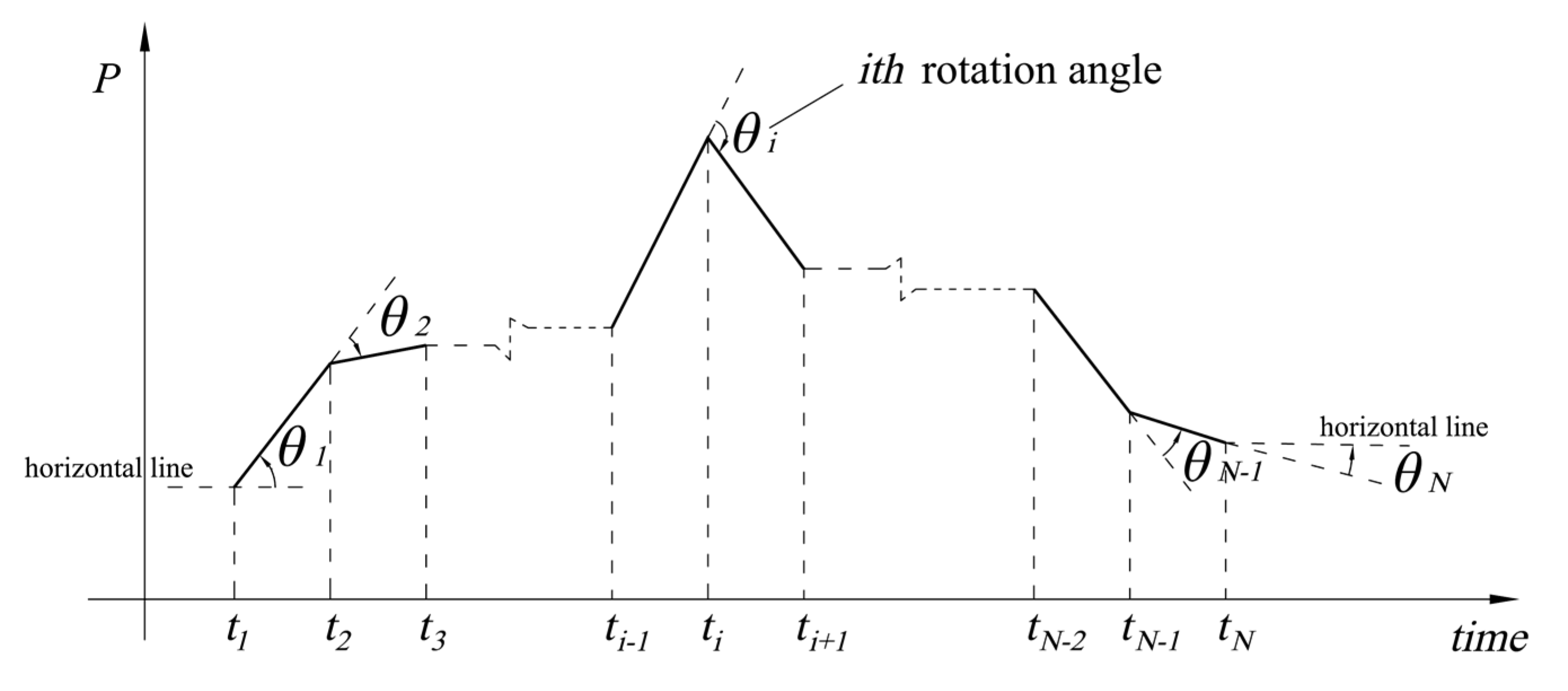
In the MWF, the rotation angles associated with a time-series of power output can be seen in a two-dimensional graph of power output vs. time, which is shown in Figure 4. For each level of power output Pi, there is an associated power output rotation angle that depends on the magnitude of power output at one time instance relative to the trend observed in the immediately previous periods. In this way, the power output rotation angle truly captures the magnitude of sudden fluctuations. Since one large rotation angle gives rise to a more noticeable fluctuation as compared to several small rotation angles (even if the sum of the small angles is equal to the value of the large angle) such as a sudden ramp up or down in output causing additional start-up and shut-down costs in the power system, the metric of short-term fluctuation used in this study takes the exponential function of each angle before adding them up.
The objective of minimizing the short-term fluctuations in total output from wind, PV, and SHP is formulated, as shown in Equations (1)–(5).
where the subscript i refers to the time interval with I = 1, 2, …, N. N is the total number of intervals in the time horizon. is the rotation angle of in the ith interval, which is shown in Figure 4 (radian). is the gradient between and (MW/h). is the total power output of SHP, wind, and PV in Area I in the ith interval (MW). is the small hydropower output in the ith interval (MW). The superscript SHP refers to small hydropower. is the wind farm output in the ith interval (MW). The superscript W refers to the wind farm. is the PV power output in the ith interval (MW). The superscript PV refers to PV power. is the maximum output of small hydropower in the ith interval, namely, the largest output that could be generated with the inflow and the water in the reservoir (MW). In addition, is the ratio of in the ith interval, which is the variable of this model and ranges from 0 to 1. The detailed definitions and calculations of the rotation angle can be found in a previous study [35].
(2) Constraints
There are commonly three types of constraints in the multi-energy optimization (i.e., resource type, grid type, and station type [36,38,39]). In this paper, the transfer capability limitation and transmission losses are not considered. Because of space limitations, only the main constraints are presented in the text. The additional constraints can be found in Appendix A.2 (Table A2, Table A3, Table A4, Table A5, Table A6, Table A7 and Table A8).
(a) Power Balance
where is the output of thermal power in the ith interval (MW). The superscript Th refers to the thermal power. is the power delivered from Area I to Area II in the ith interval (MW) and is the load in Area I in the ith interval (MW).
(b) Small hydropower
where is the generated total amount of power production from SHP in the dispatch horizon in the results of the model optimization (MWh). is the scheduled total amount of power production from SHP in the dispatch horizon (MWh). is the control value of the gap between and (MWh). is the volume of water stored in the reservoir at the beginning of the ith interval (m3). is the inflow of the reservoir in the ith interval (m3/s). is the outflow of the reservoir in the ith interval (m3/s) and is the temporal length of a single period (s).
(c) Wind power
where is the wind speed in the ith interval (m/s). is the minimum wind speed required for power generation at this wind turbine (m/s). is the maximum wind speed at which this wind turbine can generate power (m/s) and is a function that outputs the amount of electric power production from the wind turbine for a given wind speed.
(d) PV power
where is the installed capacity of PV power (MW). is the actual intensity of solar radiation in the ith interval (W/m2). is the solar radiation intensity under the standard test conditions, which is equivalent to 1000 W/m2. is the temperature coefficients of power output of the solar cell module (−0.35%/°C). is the actual temperature of the module in the ith interval (°C) and is the temperature under the standard test conditions (25 °C [40]).
(e) Thermal power
where is the minimum output of the thermal power (MW). is the maximum output of the thermal power (MW).
Taking results in the left panel of following Figure 9 in Section 5 as a simple example of multi-energy integration in Area I, it illustrates the effect of SHP on smoothing the fluctuant output from wind and PV power and denotes the surplus power production, 500.5 MWh (power production above load), caused by the high penetration of RES in Area I.
3.2. Integration in Area II
In Area II, it is assumed that (1) the power system consists of two types of power sources: PHS and non-renewable power (e.g., coal-fired thermal power and nuclear power), (2) the power production delivered from Area I is consumed in this area, and (3) the surplus power in this area will be curtailed. The presented model aims to employ PHS to shift the surplus power imported from Area I to the peak period. The PHS pumps water into its upper reservoir to store the surplus power and generate power production in the peak period in order to obtain benefits by selling the power at a high price and smooth the non-renewable power fluctuations.
(1) Objective
The aims of multi-energy integration in Area II are not only to maximize income by generating power at high prices but also to minimize the output fluctuation of non-renewable power. These two aims are combined into one objective, according to Equation (13).
The objective is formulated as shown in Equations (13)–(19).
where is the cost to pump water into the upper reservoir of the PHS system (RMB). is the income from power generation by PHS (RMB). is the output fluctuation in non-renewable power when the Area II power system operates with PHS (MW). is the output fluctuation in non-renewable power when the Area II power system operates without PHS (MW). is the input (pumping power [41]) of PHS in the ith interval (MW). is the output (generating power) of PHS in the ith interval (MW). is the power price in the ith interval (RMB/MW). is the output of non-renewable power when the Area II power system operates with PHS in the ith interval (MW). The superscript NR refers to the non-renewable power. is the average value of from the first to the Nth interval (MW). is the output of non-renewable power when the Area II power system operates without PHS in the ith interval (MW). is the average value of from the first to the Nth interval (MW). is the rotation angle of the output of the (radian). is the rotation angle of the output of (radian). is the installed PHS capacity of pumping power (MW). is the installed PHS capacity of generating power (MW) and is the ratio of the PHS power in the ith interval, which is the variable of this model and ranges from −1 to 1.
(2) Constraints
The operation of the PHS involves system balance, reservoirs, and plant operations [41]. The main constraints are listed below.
(a) Power balance
where is the import power that is delivered from Area I in the ith interval (MW) and is the load in Area II in the ith interval (MW).
(b) Reservoirs
where is the water storage in the upper reservoir of the PHS system in the ith interval (m3). is the water flow pumped into the upper reservoir of the PHS system in the ith interval (m3/s). is the water flow used to generate power from the upper reservoir of the PHS system in the ith interval (m3/s). is the water storage in the lower reservoir of the PHS system in the ith interval (m3). is the water level of the upper reservoir of the PHS system at the beginning of the dispatch horizon (m) and is the water level of the upper reservoir of the PHS system at the end of the dispatch horizon (m).
(c) PHS plants
where is the coefficient of generating power of PHS, is the water head between the upper and lower reservoirs of PHS in the ith interval (the head loss is not considered in this paper) (m), and is the coefficient of the pumping power of PHS.
(d) Non-renewable power
where is the minimum output of thermal power (MW) and is the maximum output of thermal power (MW).
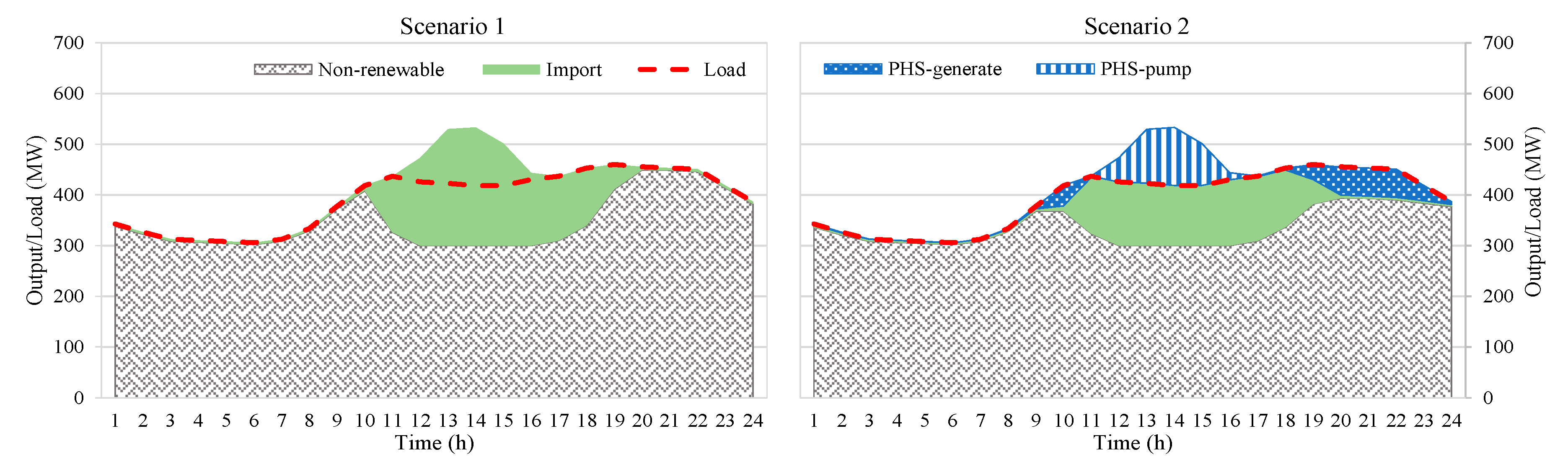
The results displayed in the right panel of Figure 11 in Section 5 could be taken as a simple example of multi-energy integration in Area II. It reflects the role of PHS in shifting the surplus power production, 365.3 MWh (PHS-pump zone), and the function of PHS to smooth the output of non-renewable power in Area II. Comparing these two simple examples in Areas I and II, the differences between integrations in Areas I and II are revealed. SHP is used to smooth the fluctuant output while PHS is employed to save the curtailment of power and smooth the fluctuant output.
4. Solution Algorithm
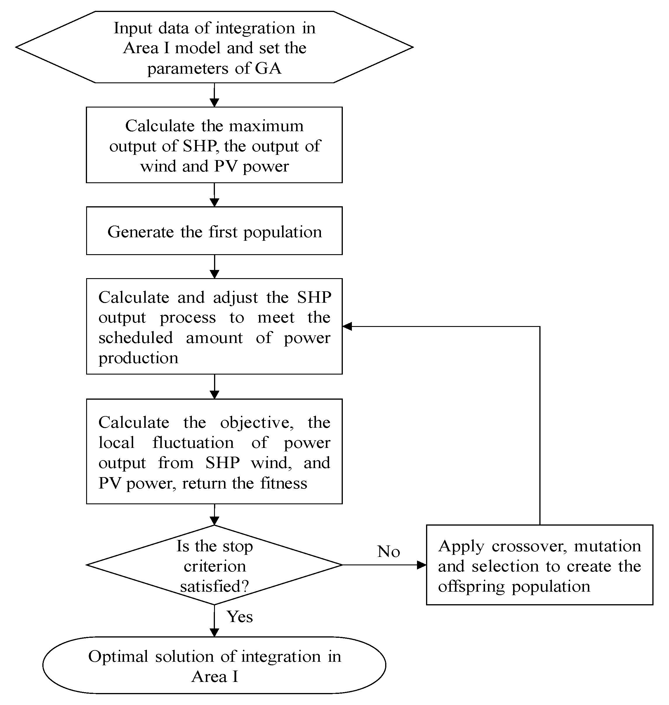
Since the fluctuations in PV power mainly exists on sub-daily time steps and the sub-daily wind power also alternates noticeably in some regions, the simulations of multi-energy integration in Area I and II are carried out over one day and its resolution is one hour. The integration in Area I is first optimized to smooth the fluctuating wind/PV power with SHP and work out the power exported to Area II, which is one basis of multi-energy integration in Area II. With the optimized results in Area I, the integration in Area II is enabled by employing PHS to shift the surplus power toward the peak period. The Genetic Algorithm Toolbox of MATLAB (https://www.mathworks.com/, R2017a version) is used to optimize the multi-energy integration by generating and improving the variable of the model, which decides the hourly output processes of SHP and PHS.
The solution procedure for multi-energy integration in Area I is completed in six steps, which is described below.
Step 1: Calculate the maximum output of SHP as well as the wind power output and PV power output based on the resource and station constraints.
Step 2: Randomly generate the first population of values representing the ratio of the maximum output of SHP (i.e., a value from 0 to 1).
Step 3: Calculate the SHP output process with and adjust the SHP output process to meet the scheduled amount of power generation by increasing or decreasing the output, which is described in Section 2.
Step 4: Evaluate the fitness of the current population. Calculate the fitness value corresponding to the objective function, as previously described in Section 3.1.
Step 5: If the stop criterion of the genetic algorithm (GA) (i.e., number of iterations/generations) is satisfied, then stop and obtain the final optimal coordinated dispatch. If not, then proceed to step 6.
Step 6: Create the offspring population (i.e., crossover, mutation, and selection [42]) and go to step 3.
The flow chart of the solution algorithm is displayed in Figure 5.
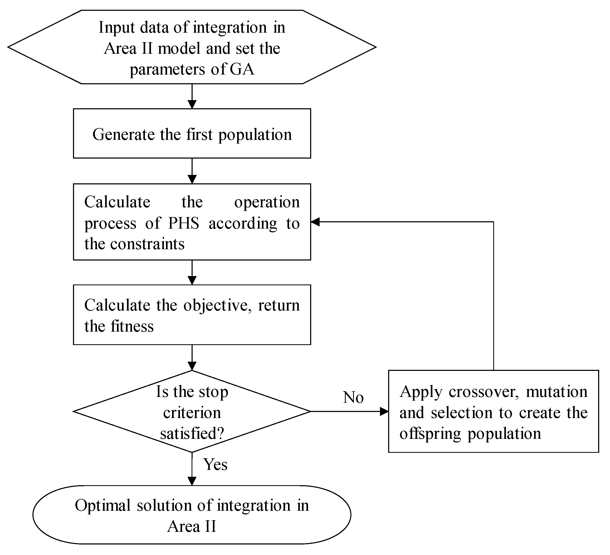
The solution procedure for multi-energy integration in Area II is completed in five steps, as described below.
Step 1: Randomly generate the first population of values representing the ratio of the pumping/generating power of PHS (i.e., a value from −1 to 1).
Step 2: Calculate the operation process with constrained by the system balance, reservoirs, and plant operation constraints.
Step 3: Evaluate the fitness of the current population. Calculate the fitness value corresponding to the objective function, which was previously described in Section 3.2.
Step 4: If the stop criterion of the GA (i.e., number of iterations/generations) is satisfied, then stop and obtain the final optimal coordinated dispatch. If not, then proceed to step 5.
Step 5: Create the offspring population (i.e., crossover, mutation, and selection) and go to step 2.
The flow chart of the solution algorithm is displayed in Figure 6.
5. Case Study
5.1. Data
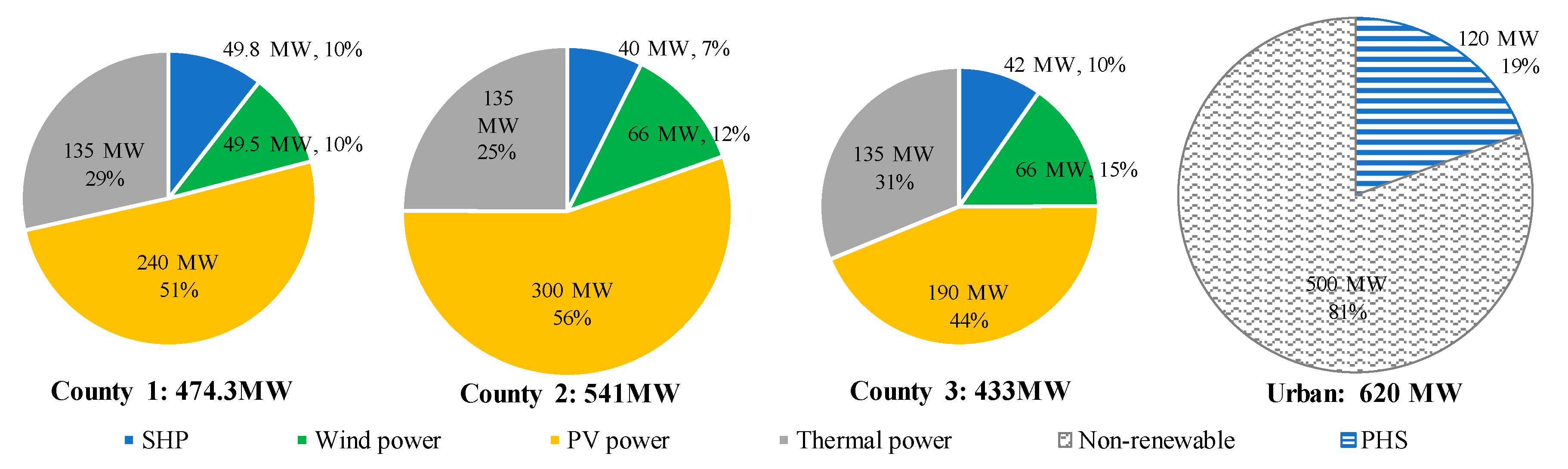
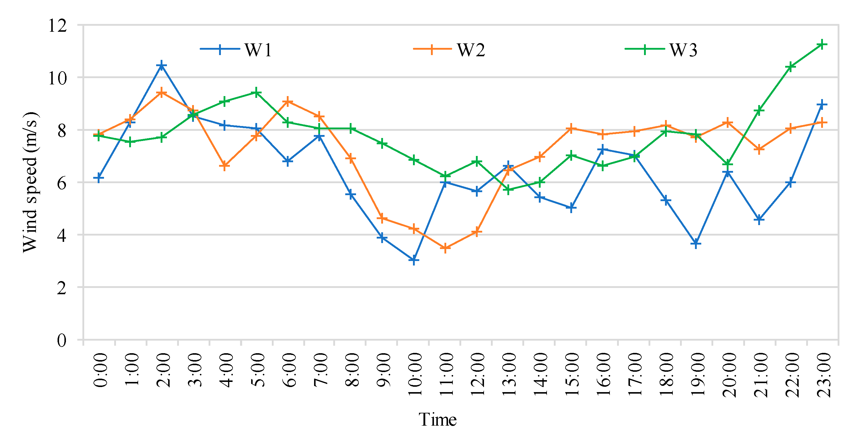
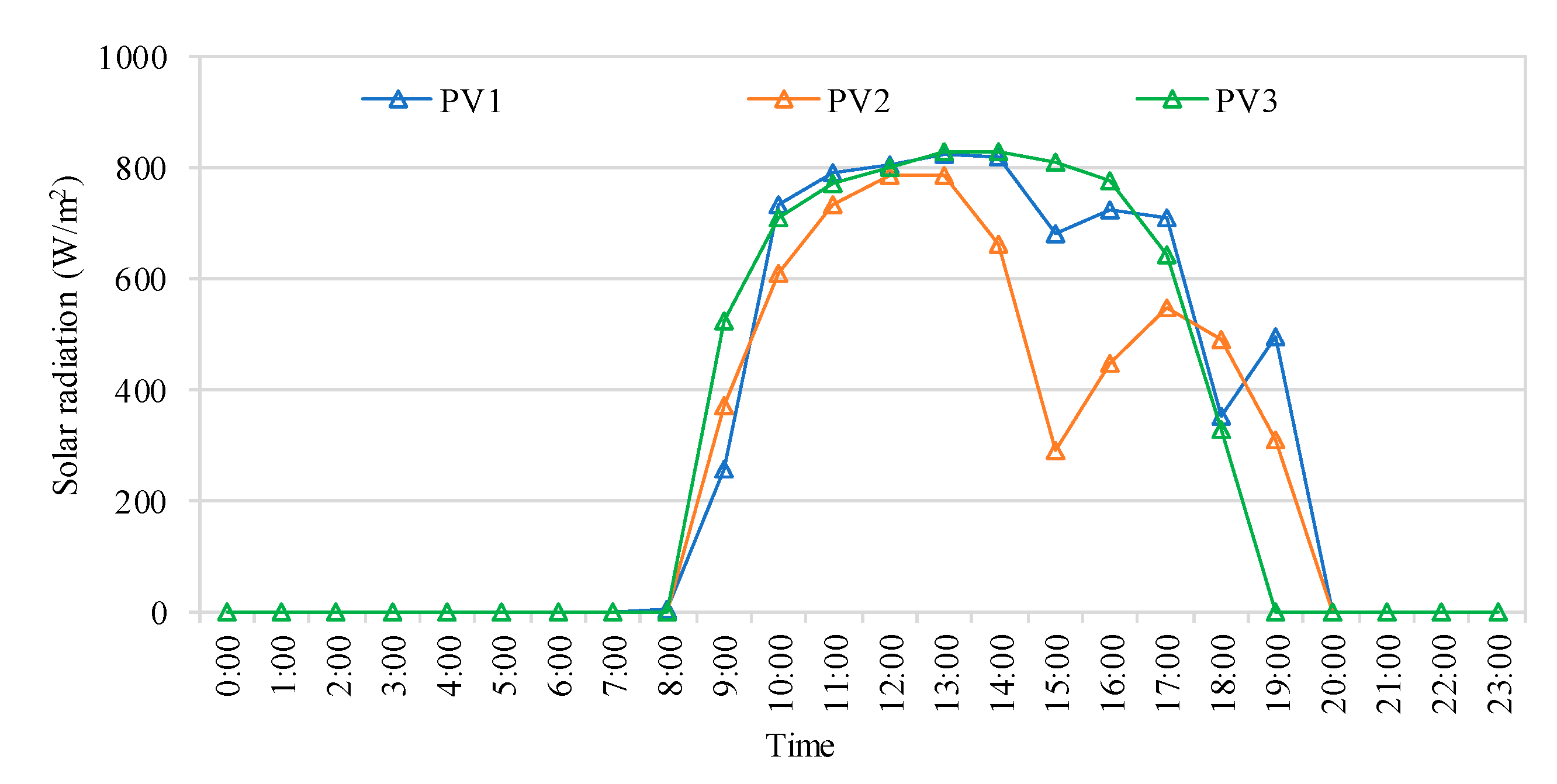
The case we studied is a virtual power system based on a municipal power system in Southwestern China. The virtual power system contains three county (remote) grids and one urban grid. The county grids include thermal power, SHP (with reservoir), wind power, and PV power. The urban grid consists of non-renewable power (e.g., thermal power and nuclear power) and PHS. The installed capacity of the power stations is displayed in Figure 7. In these county grids, the capacities of SHP are less than 50 MW and the penetrations are approximately 10%. The firm power outputs of these SHP stations are approximately 10 MW, which is 6% of the load in the respective county grid. The rapidly increasing wind/PV power causes an oversupply of power in the county and this surplus power is delivered to Area II to meet the high power demands of the urban grid. The thermal power is assumed to be coal-fired thermal power, which is one major component of the Chinese power system. The urban grid contains one PHS power source (pumping capacity: 130 MW, generating capacity: 120 MW) and several non-renewable power sources (e.g., thermal power and nuclear power).
As natural resources, runoff, wind, and solar energy have seasonal variations. For runoff, there are two typical seasons: the dry season and the flood season. In the dry season, runoff is commonly stable. It alternates drastically during the flood season. In this study, the simulation of multi-energy power system operations is conducted during the dry season with an hourly runoff/wind speed/solar radiation time series. The temporal resolution of the simulation is one hour and the temporal horizon of the simulation is one day. In the optimization, we adopted the following parameters for the genetic algorithm: the population size is 100, the crossover rate is 0.5, the mutation rate is 0.01, and the stop criterion is that either the best result remains unchanged for multiple generations or the generation number reaches 200. A summary of all data used can be found in Appendix A.1, which includes the resource time series (Figure A1, Figure A2, Figure A3 and Figure A4) and power station information (Table A1).
5.2. Results and Discussion
5.2.1. Energy Mix in Area I
Since the hourly runoff over one day during the dry season is almost constant and most of the SHP stations operate like “run-of-the-river” stations [34], the hourly output of SHP is usually invariable. In this study, we assumed that, in the non-cooperation mode (i.e., no energy mix is carried out among multiple power sources), SHP generates a constant output (2 × Pfirm). At the same time, in the cooperative mode (i.e., multi-energy mix is conducted), SHP generates flexible output ranging from minimal output (constrained by minimum ecological flow [43]) to maximal output (constrained by installed capacity) to smooth the fluctuating output from wind/PV power. Therefore, the potential ability of SHP to complement wind/PV power is explored in the cooperative mode and not in the non-cooperation mode.
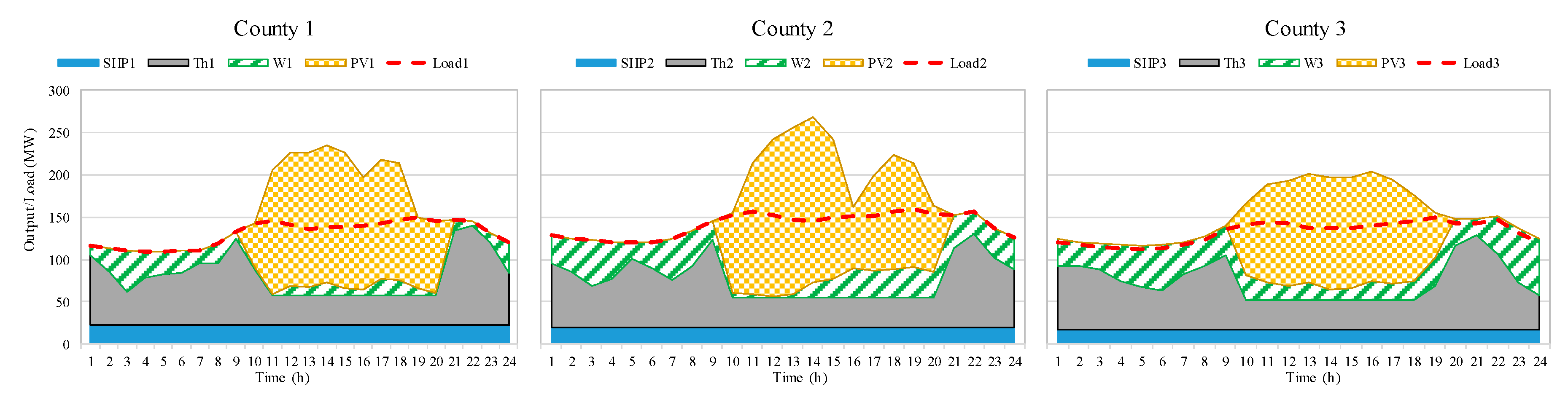
The results of the power system operation in the non-cooperation mode are displayed in Figure 8. In the non-cooperation mode, due to SHP generating a constant output, thermal power is employed to complement the intermittent output from wind/PV power to meet the power supply-demand balance (as shown in Figure 8). Since the minimal output of thermal power is relatively high (30% [44]) and the wind/PV penetration is significant (approximately 60%), an over-supply occurs (during the daytime from 11:00 to 19:00 in this case study). Frequently alternating thermal output leads to ramping up/down or start-up/shut-down operations and results in higher operation costs. In addition, although the penetration of SHP (approximately 10%) is finite, it can still be explored to smooth the fluctuating output. Thus, exploring the potential flexibility of SHP in the energy mix is feasible and necessary.
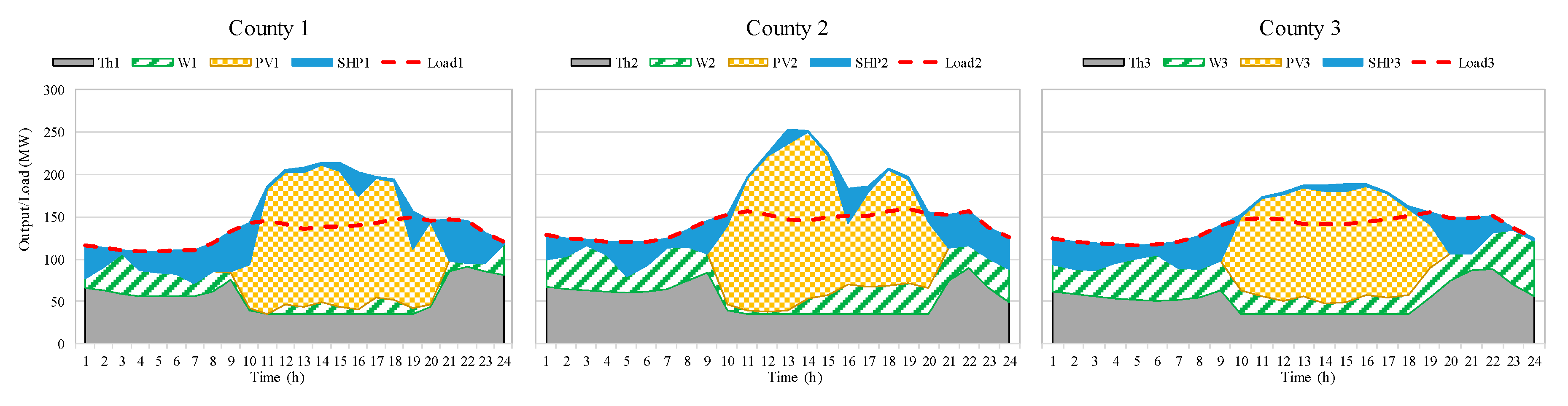
The output processes of thermal power in the cooperative mode (as shown Figure 9) are apparently smoother than those in the non-cooperation mode (Figure 8). Using County 1 as an example, the output of Th1 thermal power varies from 39 MW to 101 MW from 1:00 to 9:00 in the non-cooperation mode while the Th1 output is only slightly altered by approximately 10 MW in the cooperative mode. Similar phenomena can also be found in the first half of the night and in the other two counties.
The power production and operation costs of thermal power in the non-cooperation and cooperative modes are listed in Table 1. In all three counties, the thermal power production decreases (by approximately 110 MWh) and the operation costs decline (by approximately 28,000 RMB) when SHP is employed to complement wind/PV power. The details of the thermal power operation costs are listed in Table 2. Most of the cost reduction is attained from the fuel cost, which reflects the mitigation of thermal power production. This result occurs because part of the thermal power production is replaced by the power generated from SHP. The start-up and shut-down costs are also reduced, which results from the flatter output of thermal power smoothed by the flexible SHP. This result illustrates that employing the flexible SHP potential to complement wind/PV power (rather than employing thermal power) could replace thermal power production with renewable power production as well as smooth the thermal output and further reduce the operation costs of thermal power, which is mainly the fuel cost.
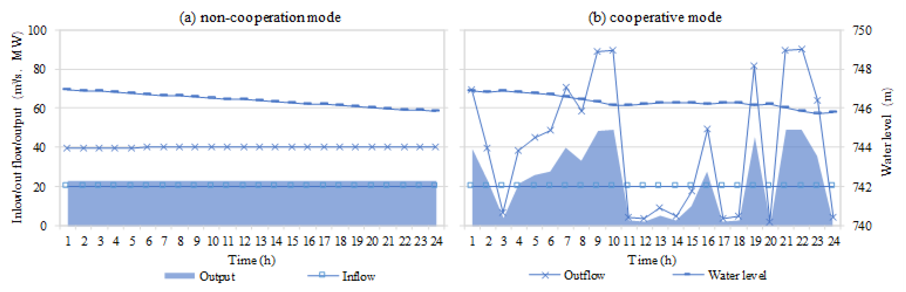
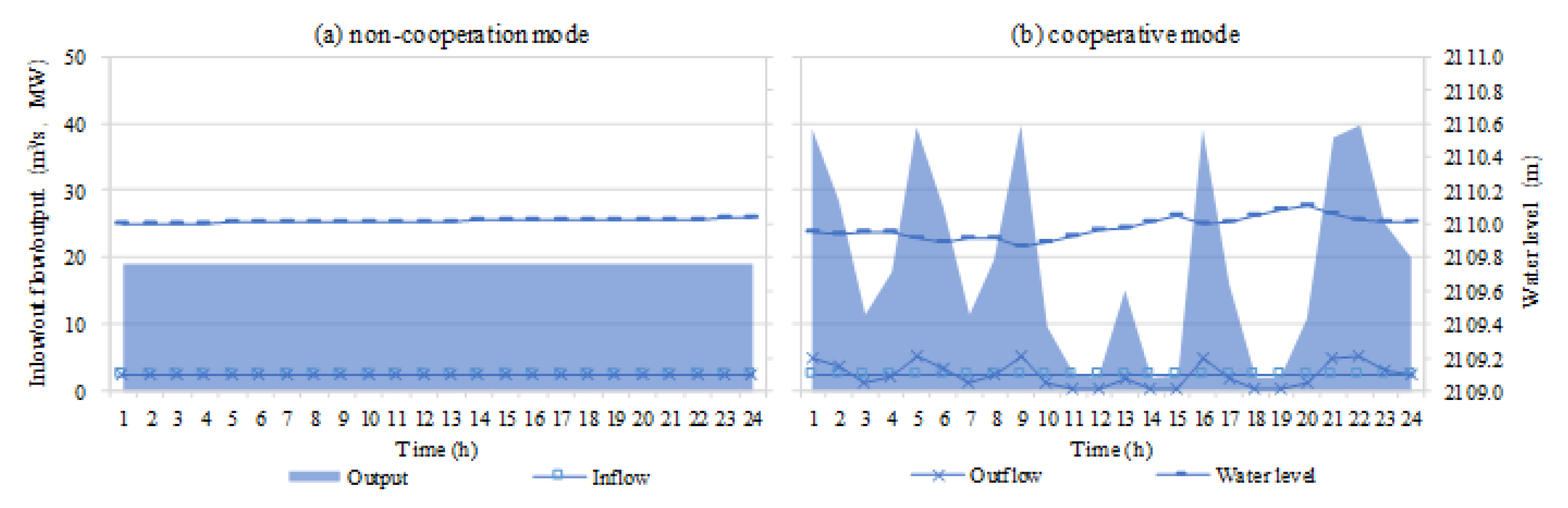
The operation processes of SHP1 are displayed in Figure 10 in terms of inflow, outflow, reservoir water level, and output. In the non-cooperation mode, SHP1 generates a stable output (22.96 MW). Thus, its outflow is almost constant (40 m3/s), and its reservoir water level gradually falls. Hydropower plants are very flexible in altering their output and range from minimal output to installed capacity. For SHP1 in the non-cooperation mode, space amounting to approximately 25 MW (its installed capacity is 49.8 MW) is available for ramping up/down its output to complement wind and PV power. This space is guaranteed with its reservoir to supply/store the water energy. Thus, no shortage/curtailment of hydropower production occurs. These advantages of hydropower are not used in the non-cooperation mode but are fully used in the cooperative mode (Figure 10b). With the method we proposed in Section 2, although the output process of SHP changes drastically, its total power production in the cooperative mode is the same (551 MW) as that in the non-cooperative mode. Similar results can also be found in the other two counties (displayed in Figure A5 and Figure A6). These results demonstrate that the proposed method is effective and further indicate that SHP is functional in complementing wind/PV power. Additionally, it is important to note that SHP is a power source that can be dispatched to a certain extent [24].
5.2.2. PHS Optimization in Area II
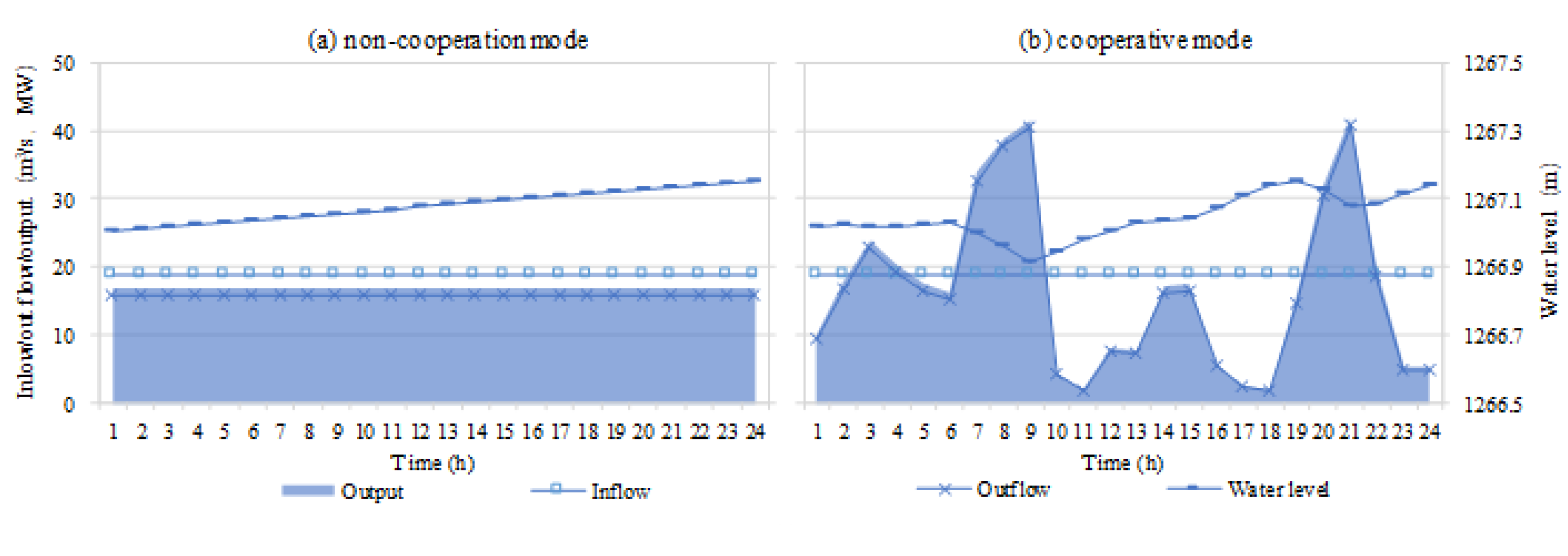
A typical operation pattern of PHS involves pumping in the off-peak period when the power supply is in surplus and generating in the peak period when the power demand is high [25]. Usually, PHS is distributed near urban areas (i.e., manufacturing bases and cities) where a large gap in the power demand occurs between off-peak and peak periods. The utility-scale wind/PV power that is distributed in Area I is delivered to Area II to meet the high power demand. Since PV power is generated in the daytime but the peak period is generated at night, the abundant PV power delivered to Area II will cause power surplus issues during the daytime and cannot help meet the peak load during the night. However, PHS is able to solve this problem by shifting the surplus power to the peak period.
To analyze the contribution of PHS as mentioned above, two scenarios (Scenario 1/2: power system integration without/with PHS) are used in the Area II power system simulation. Their results are displayed in Figure 11 and Table 3. Under Scenario 1, although most power imported from the three remote counties is consumed, there is still some noticeable surplus power (365 MWh, import power above the load, as shown in the left panel of Figure 11). The surplus power is caused by either the rapidly increasing PV power or the high minimal output of non-renewable power. Due to the power balance and absence of PHS in Scenario 1, the surplus power must be curtailed because there is no way to store this power. Thus, the economic income of the surplus power in Scenario 1 is zero.
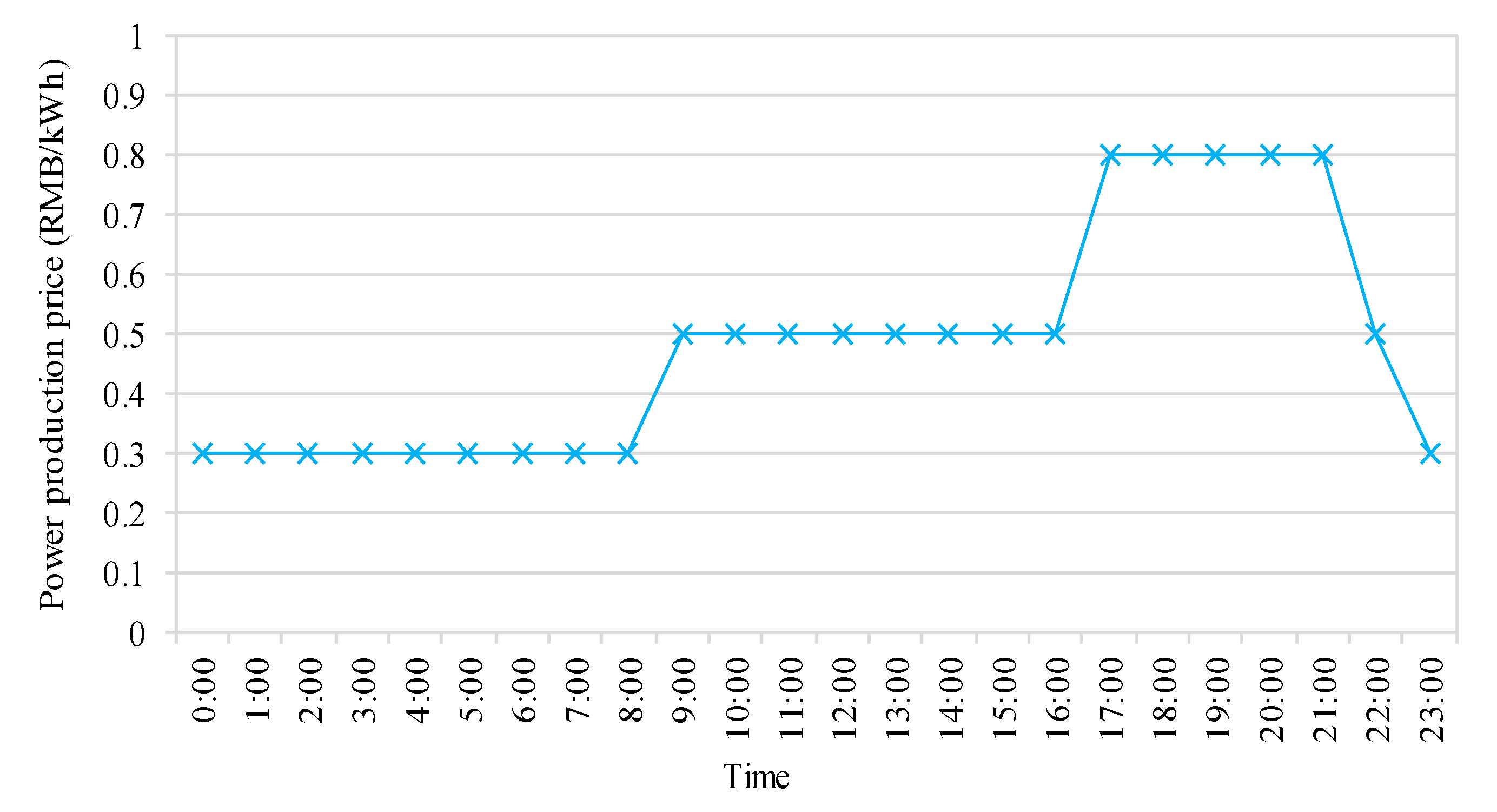
However, under Scenario 2, this curtailment could be avoided. The surplus power (365 MWh, PHS-pump section shown in the right panel of Figure 11) is used to pump water into the upper reservoir of the PHS and regenerate power (291 MWh, PHS-generate section as shown in the right panel of Figure 11) in the peak period. Even though there is approximately 74.4 MWh/20% energy loss during this procedure, it is still sensible to turn “waste” (i.e., curtailed power) into “wealth” (i.e., consumed power). In this studied case, the cost of pumping surplus power is assumed to be zero and the price of selling power to the grid during peak periods is assumed to be 0.5 RMB/kWh or 0.8 RMB/kWh (as shown in Appendix A Figure A4). Afterward, the economic income of shifting the surplus power is approximately 201,700 RMB. Although the power type in the grid cannot be identified as renewable or non-renewable, in the background of rapidly increasing wind/PV power development based on the results of the three county regions, the surplus power in Figure 11 is highly correlated to the renewable power stations. By shifting the surplus power into the peak period, the non-renewable power production is replaced with renewable production. The work by Feng et al. [46] showed that the average total life-cycle carbon emission of coal-fired/PV power are 902/63.91 g/kWh, respectively. Assuming the surplus power (365 MWh) is from PV and the non-renewable power replaced (291 MWh) is from coal-fired power, then 239 tons of carbon emission could be cut down. This result illustrates that, when surplus power occurs in the Area II power system with PHS, the PHS can store the surplus power in the upper reservoir and regenerate it during the peak period to obtain not only the economic benefit of selling the power at high prices but also the environmental benefit of replacing non-renewable power with renewable power.
6. Conclusions
Small hydropower and pumped hydropower storage are ideal members of the power system to integrate intermittent power production from wind and PV facilities. Usually, the utility scale of renewable power (e.g., hydropower, wind, and PV) is sparsely distributed in remote areas while PHS power is distributed in core areas. This paper proposes a model for the remote power system to explore the potential of SHP to smooth the short-term fluctuations in wind and PV power and a model for the power system in an urban area to employ PHS to shift the surplus power to the peak period. The first model is aimed at minimizing output fluctuations even though it is constrained by the scheduled power production and other common constraints. The objective of the second model is to maximize the income from selling surplus power at a high price and to minimize the output fluctuations in non-renewable power. In the proposed first model, the cooperative mode not only dispatches the SHP with the reciprocal output (to the wind/PV output) to smooth the fluctuation but also operates the reservoir with scheduled total power production by adjusting its output in parallel. Through the case study based on a municipal power system in Southwestern China, the results show that, with the proposed method, SHP can successfully smooth the short-term fluctuations in wind and PV power without influencing the scheduled daily total power production. SHP can also reduce the thermal power production, smooth the thermal output, and further diminish the operation costs of thermal power. In addition, employing PHS to store the surplus power in its upper reservoir and regenerate it during the peak period can achieve not only the economic benefit of selling the power at high prices but also the environmental benefit of replacing non-renewable power with renewable power.
Future work on integrating intermittent power with SHP and PHS should be extended to other special periods (i.e., flood season and ecologically sensitive periods), which have complex constraints on the output shape, water level, discharge, and more. Additional benefits and impacts of multi-energy integration should be analyzed such as environmental protection.
Author Contributions
Y.M. and X.W. conceived and designed the experiments; X.W. carried out the main research tasks and wrote the paper; L.C. and Q.C. gave the comments and advices to the paper; Y.M. and H.W. supervised the whole research.
Funding
The authors are grateful to financial support from the National Natural Science Foundation of China (51479140, 91647204).
Acknowledgments
The authors appreciate the contributions provided by Xiangyu Cong from POWERCHINA Kunming Engineering Corporation Ltd. The Program of China Postdoctoral Science Foundation (2016M600610), the Program of the Natural Science Youth Foundation of Hubei Province (ZRMS2017000495), and the Program of the National Natural Science Foundation of China (51479140, 91647204) supported the work of X.W., Q.C., Y.M., and H.W. The National Key Research and Development Program of China (2017YFC0405900), the National Natural Science Foundation of China (51669003), and the Guangxi Provincial Natural Science Foundation (AB16380284) supported Lihua Chen. Sincere gratitude is extended to the editor and anonymous reviewers for their professional comments and corrections, which greatly improved the presentation of the paper.
Conflicts of Interest
The authors declare no conflict of interest.
Appendix A
Appendix A.1. Additional Information on the Case Study
All data (except the thermal power plant parameters) were obtained through research communications with operators and planners of the grid system in Southwestern China and are listed in the tables and figures below. All data displayed in the figures are also available upon request. The thermal power plant parameters were from the published research work by Carrion and Arroyo [45]. In the county power system, Unit 6 (80 MW) and Unit 8 (55 MW) in their paper were used in this study. Details of those plants’ parameters can be found in Reference [45].

Table A1.
Parameters of the power stations.
| Zone | Facility type | Label | Installed Capacity (MW) | Normal Water Level (m) | Conservation Storage (106 m3) | Dead Water Level (m) | Firm Power Output (MW) | Inflow (m3/s) |
|---|---|---|---|---|---|---|---|---|
| County 1 | Hydropower | SHP1 | 49.8 | 748 | 9.34 | 741 | 11.48 | 20.4 |
| Wind power | W1 | 49.5 | - | - | - | - | - | |
| PV power | PV1 | 240 | - | - | - | - | - | |
| Thermal power | Th1 | 135 | - | - | - | - | - | |
| County 2 | Hydropower | SHP2 | 40 | 2115 | 3.3 | 2090 | 9.6 | 2.4 |
| Wind power | W2 | 66 | - | - | - | - | - | |
| PV power | PV2 | 300 | - | - | - | - | - | |
| Thermal power | Th2 | 135 | - | - | - | - | - | |
| County 3 | Hydropower | SHP3 | 42 | 1272 | 29.6 | 1255 | 8.49 | 19 |
| Wind power | W3 | 66 | - | - | - | - | - | |
| PV power | PV3 | 190 | - | - | - | - | - | |
| Thermal power | Th3 | 135 | - | - | - | - | - | |
| Urban | Pumped storage power | PHS | 120 (generate status) | 308 | 4.65 | 291 | - | - |
| 130 (pump status) | 94.5 | - | 94.5 | - | - | |||
| Non-renewable power (thermal power, nuclear power, and so on) | Nr | 500 | - | - | - | - | - |
Figure A1.
Wind speed of wind farm (source: POWERCHINA Kunming Engineering Corporation Ltd.).

Figure A2.
Solar radiation of the PV power station (source: POWERCHINA Kunming Engineering Corporation Ltd.).
Figure A2.
Solar radiation of the PV power station (source: POWERCHINA Kunming Engineering Corporation Ltd.).

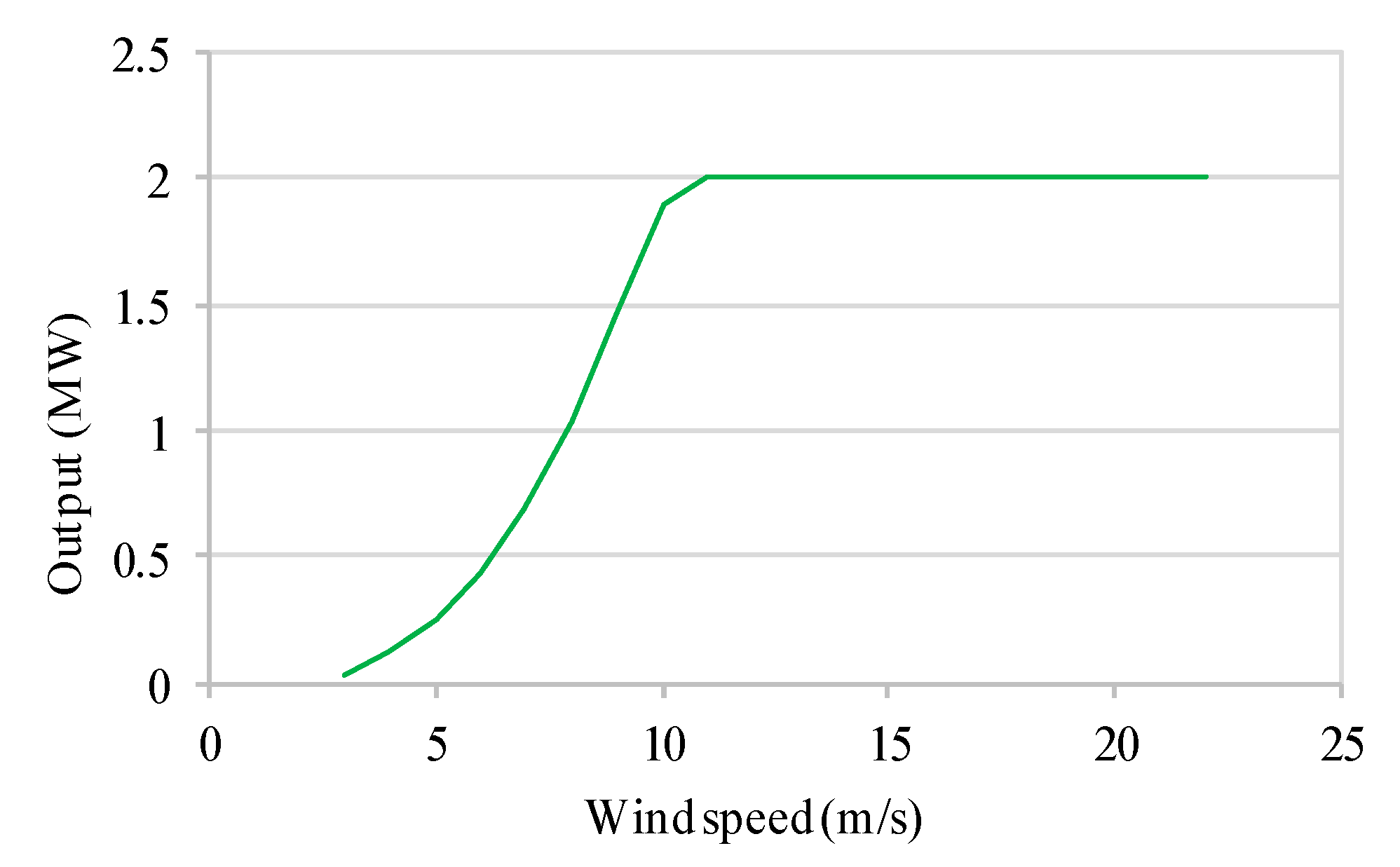
Figure A3.
Wind turbine power curve (rated capacity is 2 MW, source: POWERCHINA Kunming Engineering Corporation Ltd.).
Figure A3.
Wind turbine power curve (rated capacity is 2 MW, source: POWERCHINA Kunming Engineering Corporation Ltd.).

Figure A4.
Price of power production.

Appendix A.2. Additional Mathematical Formulation of the Proposed Model
(1) Notation
Table A2.
Abbreviations of the model of the multi-energy integration.
| Abbreviation | Description |
|---|---|
| SHP | Small hydropower |
| W | Wind power |
| PV | PV power |
| Th | Thermal power |
| NR | Non-renewable power |
(2) Additional constraints of the model of multi-energy integration in Area I
i. Resource type
Table A3.
Constraints of resources.
| Equation | Description | Scope |
|---|---|---|
| (A1) | Non-negative constraint of inflow time series | ∀ i |
| (A2) | Non-negative constraint of wind speed time series | ∀ i |
| (A3) | Non-negative constraint of solar radiation time series | ∀ i |
Table A4.
Parameters of constraints of resources.
| Parameter | Description | Unit |
|---|---|---|
| Inflow in the ith interval | m3/s | |
| Wind speed in the ith interval | m/s | |
| Solar radiation in the ith interval | W/m2 |
ii. Station type
Table A5.
Constraints of the power station.
| Equation | Description | Scope |
|---|---|---|
| (A4) | Range of outflow | ∀ i |
| (A5) | Range of volume of water stored in the reservoir | ∀ i |
| (A6) | Range of output of the hydropower | ∀ i |
| (A7) | Limitation of the output increase of hydropower | ∀ |
| (A8) | Limitation of output decrease of hydropower | ∀ |
| (A9) | Range of output of the wind farm | ∀ i |
| (A10) | Limitation of the output increase of the wind farm | ∀ |
| (A11) | Limitation of output decrease of the wind farm | ∀ |
| (A12) | Range of output of PV power | ∀ i |
| (A13) | Limitation of output increase of PV power | ∀ |
| (A14) | Limitation of output decrease of PV power | ∀ |
| (A15) | Limitation of output increase of thermal power | ∀ |
| (A16) | Limitation of output decrease of thermal power | ∀ |
Table A6.
Parameters of constraints of the power station.
| Parameter | Description | Unit |
|---|---|---|
| Volume of water was stored in the reservoir at the beginning of the ith interval | m3 | |
| Inflow of the reservoir in the ith interval | m3/s | |
| Outflow of the reservoir in the ith interval | m3/s | |
| Maximum of *, which is a wildcard that represents a certain parameter mentioned in this paper | - | |
| Minimum of *, which is a wildcard that represents a certain parameter mentioned in this paper | - | |
| Limitation of output increase of SHP | MW | |
| Limitation of output decrease of SHP | MW | |
| Limitation of output increase of the wind farm | MW | |
| Limitation of output decrease of the wind farm | MW | |
| Limitation of output increase of PV power | MW | |
| Limitation of output decrease of PV power | MW | |
| Limitation of output increase of thermal power | MW | |
| Limitation of output decrease of thermal power | MW |
(3) Additional constraints of the model of multi-energy integration in Area II
Table A7.
Constraints of the power station.
| Equation | Description | Scope |
|---|---|---|
| (A17) | Range of output of PHS | ∀ i |
| (A18) | Limitation of output increase of PHS | ∀ |
| (A19) | Limitation of output decrease of PHS | ∀ |
| (A20) | Range of input of PHS | ∀ i |
| (A21) | Limitation of input increase of PHS | ∀ |
| (A22) | Limitation of input decrease of PHS | ∀ |
| (A23) | Limitation of output increase of non-renewable power | ∀ |
| (A24) | Limitation of output decrease of non-renewable power | ∀ |
Table A8.
Parameters of constraints of the power station.
| Parameter | Description | Unit |
|---|---|---|
| Limitation of the output increase of PHS | MW | |
| Limitation of the output decrease of PHS | MW | |
| Limitation of the input increase of PHS | MW | |
| Limitation of the input decrease of PHS | MW | |
| Limitation of the output increase of non-renewable power | MW | |
| Limitation of the output decrease of non-renewable power | MW |
Appendix A.3. Additional Results
Figure A5.
Operation process of SHP2 in County 2.

Figure A6.
Operation process of SHP3 in County 3.

References
- IPCC. Special Report on Global Warming of 1.5 °C approved by governments. Summary for Policy-Makers, Incheon, Korea, 2018. [Google Scholar]
- IPCC. Special report on renewable energy sources and climate change mitigation. Summary for Policy-Makers, Budapest, Hungary, 2011. [Google Scholar]
- Yang, W.J.; Norrlund, P.; Saarinen, L.; Witt, A.; Smith, B.; Yang, J.D.; Lundin, U. Burden on hydropower units for short-term balancing of renewable power systems. Nat. Commun. 2018, 9, 2633. [Google Scholar] [CrossRef] [PubMed]
- Francois, B.; Borga, M.; Anquetin, S.; Creutin, J.D.; Engeland, K.; Favre, A.C.; Hingray, B.; Ramos, M.H.; Raynaud, D.; Renard, B.; et al. Integrating hydropower and intermittent climate-related renewable energies: A call for hydrology. Hydrol. Process. 2014, 28, 5465–5468. [Google Scholar] [CrossRef]
- Ellabban, O.; Abu-Rub, H.; Blaabjerg, F. Renewable energy resources: Current status, future prospects and their enabling technology. Renew. Sustain. Energy Rev. 2014, 39, 748–764. [Google Scholar] [CrossRef]
- Manzano-Agugliaro, F.; Taher, M.; Zapata-Sierra, A.; Juaidi, A.; Montoya, F.G. An overview of research and energy evolution for small hydropower in Europe. Renew. Sustain. Energy Rev. 2017, 75, 476–489. [Google Scholar] [CrossRef]
- Kougias, I.; Szabo, S. Pumped hydroelectric storage utilization assessment: Forerunner of renewable energy integration or Trojan horse? Energy 2017, 140, 318–329. [Google Scholar] [CrossRef]
- Inman, R.H.; Pedro, H.T.C.; Coimbra, C.F.M. Solar forecasting methods for renewable energy integration. Prog. Energy Combust. Sci. 2013, 39, 535–576. [Google Scholar] [CrossRef]
- Tsai, S.B.; Xue, Y.Z.; Zhang, J.Y.; Chen, Q.; Liu, Y.B.; Zhou, J.; Dong, W.W. Models for forecasting growth trends in renewable energy. Renew. Sustain. Energy Rev. 2017, 77, 1169–1178. [Google Scholar] [CrossRef]
- Beluco, A.; Kroeff de Souza, P.; Krenzinger, A. A method to evaluate the effect of complementarity in time between hydro and solar energy on the performance of hybrid hydro PV generating plants. Renew. Energy 2012, 45, 24–30. [Google Scholar] [CrossRef]
- Solomon, A.A.; Kammen, D.M.; Callaway, D. Investigating the impact of wind-solar complementarities on energy storage requirement and the corresponding supply reliability criteria. Appl. Energy 2016, 168, 130–145. [Google Scholar] [CrossRef]
- Barton, J.P.; Infield, D.G. Energy storage and its use with intermittent renewable energy. IEEE Trans. Energy Convers. 2004, 19, 441–448. [Google Scholar] [CrossRef]
- Castillo, A.; Gayme, D.F. Grid-scale energy storage applications in renewable energy integration: A survey. Energy Convers. Manag. 2014, 87, 885–894. [Google Scholar] [CrossRef]
- Ji, B.; Yuan, X.H.; Li, X.S.; Huang, Y.H.; Li, W.W. Application of quantum-inspired binary gravitational search algorithm for thermal unit commitment with wind power integration. Energy Convers. Manag. 2014, 87, 589–598. [Google Scholar] [CrossRef]
- Becker, S.; Rodriguez, R.A.; Andresen, G.B.; Schramm, S.; Greiner, M. Transmission grid extensions during the build-up of a fully renewable pan-European electricity supply. Energy 2014, 64, 404–418. [Google Scholar] [CrossRef] [Green Version]
- Liu, Z. Global Energy Interconnection; Academic Press Ltd-Elsevier Science Ltd.: London, UK, 2015; pp. 1–379. [Google Scholar]
- Tabatabaee, S.; Mortazavi, S.S.; Niknam, T. Stochastic scheduling of local distribution systems considering high penetration of plug-in electric vehicles and renewable energy sources. Energy 2017, 121, 480–490. [Google Scholar] [CrossRef]
- Esther, B.P.; Kumar, K.S. A survey on residential Demand Side Management architecture, approaches, optimization models and methods. Renew. Sustain. Energy Rev. 2016, 59, 342–351. [Google Scholar] [CrossRef]
- François, B.; Hingray, B.; Raynaud, D.; Borga, M.; Creutin, J.D. Increasing climate-related-energy penetration by integrating run-of-the river hydropower to wind/solar mix. Renew. Energy 2016, 87, 686–696. [Google Scholar] [CrossRef]
- Lopes, V.S.; Borges, C.L.T. Impact of the Combined Integration of Wind Generation and Small Hydropower Plants on the System Reliability. IEEE Trans. Sustain. Energy 2015, 6, 1169–1177. [Google Scholar] [CrossRef]
- Kougias, I.; Szabó, S.; Monforti-Ferrario, F.; Huld, T.; Bódis, K. A methodology for optimization of the complementarity between small-hydropower plants and solar PV systems. Renew. Energy 2016, 87, 1023–1030. [Google Scholar] [CrossRef]
- Soulis, K.X.; Manolakos, D.; Anagnostopoulos, J.; Papantonis, D. Development of a geo-information system embedding a spatially distributed hydrological model for the preliminary assessment of the hydropower potential of historical hydro sites in poorly gauged areas. Renew. Energy 2016, 92, 222–232. [Google Scholar] [CrossRef]
- François, B.; Zoccatelli, D.; Borga, M. Assessing small hydro/solar power complementarity in ungauged mountainous areas: A crash test study for hydrological prediction methods. Energy 2017, 127, 716–729. [Google Scholar] [CrossRef]
- Jurasz, J.; Ciapala, B. Integrating photovoltaics into energy systems by using a run-off-river power plant with pondage to smooth energy exchange with the power gird. Appl. Energy 2017, 198, 21–35. [Google Scholar] [CrossRef]
- Rehman, S.; Al-Hadhrami, L.M.; Alam, M.M. Pumped hydro energy storage system: A technological review. Renew. Sustain. Energy Rev. 2015, 44, 586–598. [Google Scholar] [CrossRef]
- Katsaprakakis, D.A.; Christakis, D.G.; Zervos, A.; Papantonis, D.; Voutsinas, S. Pumped storage systems introduction in isolated power production systems. Renew. Energy 2008, 33, 467–490. [Google Scholar] [CrossRef]
- Varkani, A.K.; Daraeepour, A.; Monsef, H. A new self-scheduling strategy for integrated operation of wind and pumped-storage power plants in power markets. Appl. Energy 2011, 88, 5002–5012. [Google Scholar] [CrossRef]
- Ma, T.; Yang, H.; Lu, L.; Peng, J. Pumped storage-based standalone photovoltaic power generation system: Modeling and techno-economic optimization. Appl. Energy 2015, 137, 649–659. [Google Scholar] [CrossRef]
- Katsaprakakis, D.A.; Christakis, D.G.; Pavlopoylos, K.; Stamataki, S.; Dimitrelou, I.; Stefanakis, I.; Spanos, P. Introduction of a wind powered pumped storage system in the isolated insular power system of Karpathos–Kasos. Appl. Energy 2012, 97, 38–48. [Google Scholar] [CrossRef]
- Jurasz, J.; Dabek, P.B.; Kazmierczak, B.; Kies, A.; Wdowikowski, M. Large scale complementary solar and wind energy sources coupled with pumped-storage hydroelectricity for Lower Silesia (Poland). Energy 2018, 161, 183–192. [Google Scholar] [CrossRef]
- Canales, F.A.; Beluco, A.; Mendes, C.A.B. A comparative study of a wind hydro hybrid system with water storage capacity: Conventional reservoir or pumped storage plant? J. Energy Storage 2015, 4, 96–105. [Google Scholar] [CrossRef]
- UNIDO. ICSHP World Small Hydropower Development Report 2016; United Nations Industrial Development Organization International Center on Small Hydro Power: Vienna Hangzhou, 2016. [Google Scholar]
- IRENA. Electricity Storage and Renewables: Costs and Markets to 2030; International Renewable Energy Agency: Abu Dhabi, United Arab Emirates, 2017. [Google Scholar]
- Cheng, C.T.; Liu, B.X.; Chau, K.W.; Li, G.; Liao, S.L. China’s small hydropower and its dispatching management. Renew. Sustain. Energy Rev. 2015, 42, 43–55. [Google Scholar] [CrossRef]
- Wang, X.; Mei, Y.; Cai, H.; Cong, X. A new fluctuation index: Characteristics and application to hydro-wind systems. Energies 2016, 9, 1–17. [Google Scholar] [CrossRef]
- Wang, X.; Mei, Y.; Kong, Y.; Lin, Y.; Wang, H. Improved multi-objective model and analysis of the coordinated operation of a hydro-wind-photovoltaic system. Energy 2017, 134, 813–839. [Google Scholar] [CrossRef]
- Baker, D.B.; Richards, R.P.; Loftus, T.T.; Kramer, J.W. A new flashiness index: Characteristics and applications to midwestern rivers and streams. J. Am. Water Resour. Assoc. 2004, 40, 503–522. [Google Scholar] [CrossRef]
- Wu, X.-Y.; Cheng, C.-T.; Shen, J.-J.; Luo, B.; Liao, S.-L.; Li, G. A multi-objective short term hydropower scheduling model for peak shaving. Int. J. Electr. Power Energy Syst. 2015, 68, 278–293. [Google Scholar] [CrossRef]
- Labadie, J.W. Optimal operation of multireservoir systems: State-of-the-art review. J. Water Resour. Plan. Manag. 2004, 130, 93–111. [Google Scholar] [CrossRef]
- Ming, B.; Liu, P.; Guo, S.; Zhang, X.; Feng, M.; Wang, X. Optimizing utility-scale photovoltaic power generation for integration into a hydropower reservoir by incorporating long- and short-term operational decisions. Appl. Energy 2017, 204, 432–445. [Google Scholar] [CrossRef]
- Cheng, C.T.; Cheng, X.; Shen, J.J.; Wu, X.Y. Short-term peak shaving operation for multiple power grids with pumped storage power plants. Int. J. Electr. Power Energy Syst. 2015, 67, 570–581. [Google Scholar] [CrossRef]
- Man, K.F.; Tang, K.S.; Kwong, S. Genetic algorithms: Concepts and applications. IEEE Trans. Ind. Electron. 1996, 43, 519–534. [Google Scholar] [CrossRef]
- Fanaian, S.; Graas, S.; Jiang, Y.; van der Zaag, P. An ecological economic assessment of flow regimes in a hydropower dominated river basin: The case of the lower Zambezi River, Mozambique. Sci. Total Environ. 2015, 505, 464–473. [Google Scholar] [CrossRef]
- Gonzalez-Salazar, M.A.; Kirsten, T.; Prchlik, L. Review of the operational flexibility and emissions of gas- and coal-fired power plants in a future with growing renewables. Renew. Sustain. Energy Rev. 2018, 82, 1497–1513. [Google Scholar] [CrossRef]
- Carrion, M.; Arroyo, J.M. A computationally efficient mixed-integer linear formulation for the thermal unit commitment problem. IEEE Trans. Power Syst. 2006, 21, 1371–1378. [Google Scholar] [CrossRef]
- Feng, K.; Hubacek, K.; Siu, Y.L.; Li, X. The energy and water nexus in Chinese electricity production: A hybrid life cycle analysis. Renew. Sustain. Energy Rev. 2014, 39, 342–355. [Google Scholar] [CrossRef] [Green Version]
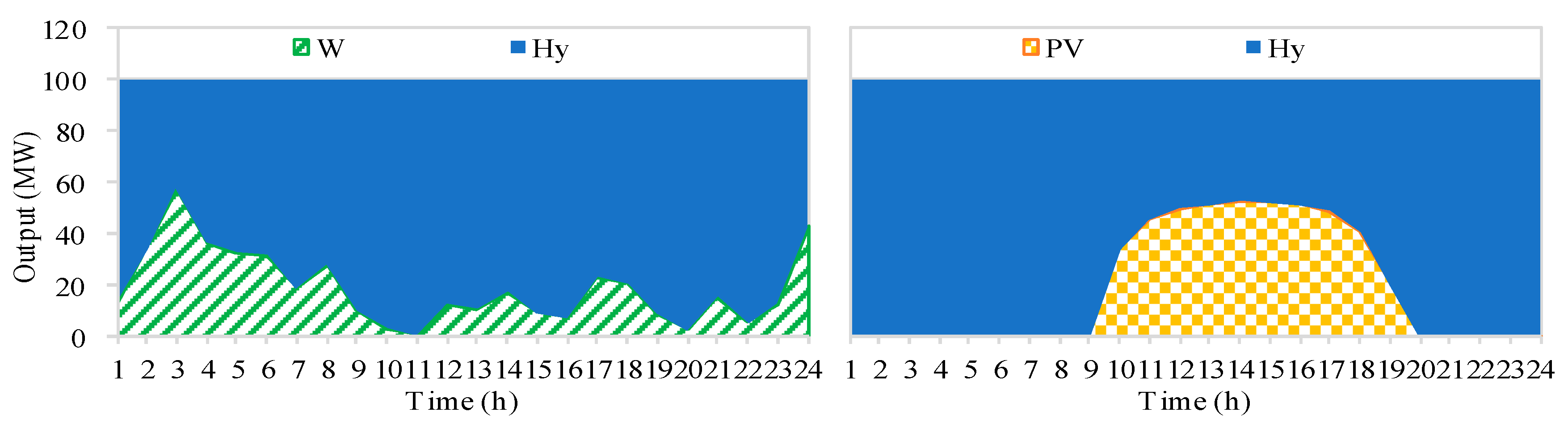
Figure 1.
Reciprocal output processes of hydropower and wind/PV power. W refers to wind power, Hy refers to hydropower, and PV refers to PV power. The value of the combined output from hydropower, wind, and PV power, 100 MW, is an example value and could be replaced by other values. It is assumed that the flat (i.e., smoothest) combined output process of hydropower and wind/PV power is the ideal combined output. In addition, in a power system possessing only hydropower and wind/PV power, the ideal combined power output is equal to the power consumption.

Figure 2.
Diagram illustrating the hydropower output process being uniformly decreased by 30 MW (assuming that decreasing the hydropower output by 30 MW would reduce the generation amount gap and the hydropower minimum output is 35 MW). (a) Hydropower output processes before the decrease and after being decreased. (b) Wind power output were combined with the hydropower output processes in the left panel. This is limited by the minimum output. The hydropower output at 3:00 and 24:00 cannot be reduced lower than 35 MW.

Figure 3.
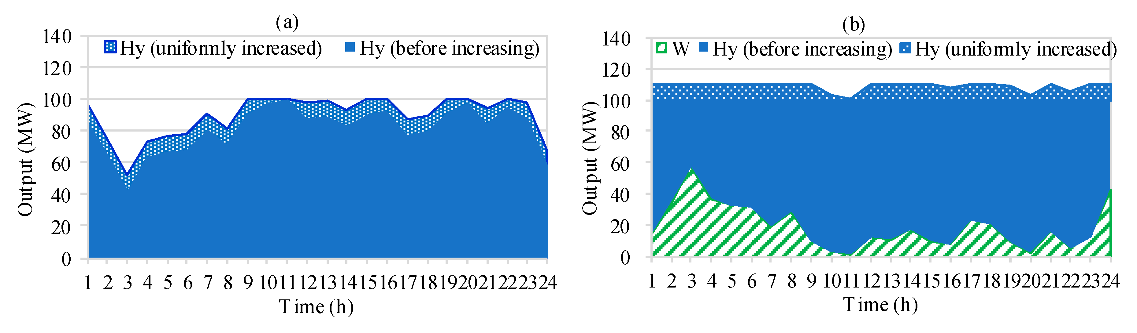
Diagram illustrating the hydropower output process being uniformly increased by 10 MW (assuming that increasing the hydropower output by 10 MW would reduce the generation amount gap and the hydropower maximum output is 100 MW). (a) Hydropower output processes before the increase and after being increased. (b) Wind power output combined with hydropower output processes in the left panel. Limited by the maximum output, the hydropower output at 10:00, 11:00, 15:00, 16:00, 19:00, 20:00, and 22:00 cannot be increased to larger than 100 MW.
Figure 3.
Diagram illustrating the hydropower output process being uniformly increased by 10 MW (assuming that increasing the hydropower output by 10 MW would reduce the generation amount gap and the hydropower maximum output is 100 MW). (a) Hydropower output processes before the increase and after being increased. (b) Wind power output combined with hydropower output processes in the left panel. Limited by the maximum output, the hydropower output at 10:00, 11:00, 15:00, 16:00, 19:00, 20:00, and 22:00 cannot be increased to larger than 100 MW.

Figure 4.
Schematic diagram of the rotation angles and line segments of the output process.

Figure 5.
Flow chart of the model decomposition in Area I.

Figure 6.
Flow chart of the model decomposition in Area II.

Figure 7.
Installed capacity of the power stations.

Figure 8.
Output process of the county power stations in counties in the non-cooperation mode.

Figure 9.
Output process of the county power stations in the cooperative mode.

Figure 10.
Operation process of SHP1 in County 1.

Figure 11.
Operation process of the power stations in Area II.

Table 1.
Power production and operation costs of thermal power.
| Region | Power Generation (MWh) | Operation Cost (RMB) | ||||
|---|---|---|---|---|---|---|
| Non-Cooperation Mode | Cooperative Mode | Difference | Non-Cooperation Mode | Cooperative Mode | Difference | |
| County 1 | 1406 | 1287 | −118 | 316,878 | 298,202 | −18,676 |
| County 2 | 1379 | 1270 | −108 | 319,533 | 290,817 | −28,716 |
| County 3 | 1368 | 1247 | −121 | 317,052 | 281,642 | −35,410 |
Note: the operation costs of thermal power in this paper are calculated with the methods and parameters published in Reference [45].
Table 2.
Detailed operation costs of thermal power.
| Region | Mode | Fuel Cost | Start-Up Cost | Shut-Down Cost | Total Cost |
|---|---|---|---|---|---|
| County 1 | Non-cooperation | 44,876 | 320 | 72 | 45,268 |
| Cooperative | 42,232 | 320 | 48 | 42,600 | |
| Difference | −2644 | 0 | −24 | −2668 | |
| County 2 | Non-cooperation | 45,172 | 380 | 96 | 45,648 |
| Cooperative | 41,153 | 320 | 72 | 41,545 | |
| Difference | −4018 | −60 | −24 | −4102 | |
| County 3 | Non-cooperation | 44,901 | 320 | 72 | 45,293 |
| Cooperative | 39,927 | 260 | 48 | 40,235 | |
| Difference | −4975 | −60 | −24 | −5059 | |
| Total | Non-cooperation | 134,949 | 1020 | 240 | 136,209 |
| Cooperative | 123,312 | 900 | 168 | 124,380 | |
| Difference | −11,637 | −120 | −72 | −11,829 |
Table 3.
Operation results of Scenario 1 and 2.
| Items | Power Generation (MWh) | Curtailment (MWh) | ||
|---|---|---|---|---|
| Non-Renewable | Import | PHS-Generate | ||
| Scenario 1 | 8332 | 1085 | 0 | 365 |
| Scenario 2 | 8041 | 1450 | 291 | 0 |
| Difference | −291 | 365 | 291 | −365 |
© 2018 by the authors. Licensee MDPI, Basel, Switzerland. This article is an open access article distributed under the terms and conditions of the Creative Commons Attribution (CC BY) license (http://creativecommons.org/licenses/by/4.0/).
Share and Cite
MDPI and ACS Style
Wang, X.; Chen, L.; Chen, Q.; Mei, Y.; Wang, H. Model and Analysis of Integrating Wind and PV Power in Remote and Core Areas with Small Hydropower and Pumped Hydropower Storage. Energies 2018, 11, 3459. https://doi.org/10.3390/en11123459
AMA Style
Wang X, Chen L, Chen Q, Mei Y, Wang H. Model and Analysis of Integrating Wind and PV Power in Remote and Core Areas with Small Hydropower and Pumped Hydropower Storage. Energies. 2018; 11(12):3459. https://doi.org/10.3390/en11123459
Chicago/Turabian StyleWang, Xianxun, Lihua Chen, Qijuan Chen, Yadong Mei, and Hao Wang. 2018. "Model and Analysis of Integrating Wind and PV Power in Remote and Core Areas with Small Hydropower and Pumped Hydropower Storage" Energies 11, no. 12: 3459. https://doi.org/10.3390/en11123459
Note that from the first issue of 2016, this journal uses article numbers instead of page numbers. See further details here.