A Novel Approach for an MPPT Controller Based on the ADALINE Network Trained with the RTRL Algorithm


Facultad de Ingeniería, Universidad del Magdalena, Santa Marta 470003, Colombia
*
Authors to whom correspondence should be addressed.
Energies 2018, 11(12), 3407; https://doi.org/10.3390/en11123407
Submission received: 9 November 2018
/
Revised: 27 November 2018
/
Accepted: 27 November 2018
/
Published: 5 December 2018
Abstract
:The Real-Time Recurrent Learning Gradient (RTRL) algorithm is characterized by being an online learning method for training dynamic recurrent neural networks, which makes it ideal for working with non-linear control systems. For this reason, this paper presents the design of a novel Maximum Power Point Tracking (MPPT) controller with an artificial neural network type Adaptive Linear Neuron (ADALINE), with Finite Impulse Response (FIR) architecture, trained with the RTRL algorithm. With this same network architecture, the Least Mean Square (LMS) algorithm was developed to evaluate the results obtained with the RTRL controller and then make comparisons with the Perturb and Observe (P&O) algorithm. This control method receives as input signals the current and voltage of a photovoltaic module under sudden changes in operating conditions. Additionally, the efficiency of the controllers was appraised with a fuzzy controller and a Nonlinear Autoregressive Network with Exogenous Inputs (NARX) controller, which were developed in previous investigations. It was concluded that the RTRL controller with adaptive training has better results, a faster response, and fewer bifurcations due to sudden changes in the input signals, being the ideal control method for systems that require a real-time response.
1. Introduction
Due to the negative impact caused by the use of conventional energy sources, environmental problems such as pollution, and poor quality in the provision of primary energy service, renewable energy is presented as an excellent alternative to reduce dependence on conventional electrical network. The notable increase in the use of renewable energies as an alternative means of generating and storing clean energy is considered worldwide as one of the technological solutions to mitigate climate change.
Internationally it is recommended that in places with high solar density, the use of photovoltaic (PV) energy sources be chosen, since this type of energy provides an inexhaustible energy resource [1]. In the global report presented in 2017 by the International Agency for Renewable Energy (IRENA), it is evident that solar energy is a leader in power generation capacity due to its competitive costs in many emerging markets of the world [2].
In order to improve competitiveness, increase demand, and obtain the highest performance, the elements of a PV system must be optimized. There are several techniques to increase the performance of PV systems, among which solar trackers [3,4,5,6,7], hybrid systems [8,9], and controllers for the maximum power point tracking (MPPT) stand out. With the MPPT controllers, better performance of the PV systems is obtained, since they take advantage of all the current generated by the solar panels independently of the voltage. These controllers are more expensive than Pulse-Width Modulation (PWM) controllers, but due to their high efficiency they are ideal for working in medium and large solar power plants [10].
In these controllers, the perturb and observe (P&O) algorithm has traditionally been used. This algorithm is characterized by its low efficiency and presenting oscillations around the operating point. The presence of oscillations has contributed to the researchers focusing their efforts on designing MPPT controllers [10] with better performance. In this way, investigations have been carried out with genetic algorithms [11], fuzzy logic [12,13,14,15,16,17], golden section [18,19], simulated annealing [20], artificial bee colony [21], adaptive control [22], glowworm swarm optimization [23], ant colony optimization [24], artificial neural networks [25,26,27,28,29,30], and numerical methods [31].
Taking into account the previous context, this paper proposes as a novelty the design of an MPPT neuro-controller based on an adaptive neural network (ADALINE) with Real-Time Recurrent Learning (RTRL) [32]. We decided to explore the application of this method in order to design a robust controller that adapts to sudden climatic changes to which a PV module will be exposed.
Specifically, we highlight as a contribution the application of the RTRL algorithm in an MPPT controller, which was developed with a single neuron and without using the bias. In addition, this training algorithm was programmed online with the Simulink function blocks without using the MATLAB Neural Network Toolbox (R2017b Version 9.3). In this way, it was possible to develop an efficient controller with excellent computing times.
The results obtained show the advantage of the use of an online learning method in an artificial neural network (ANN), with which the volume of data to be acquired and the times of capture and conditioning of the data are reduced. In addition, the controller is more flexible since it has the ability to learn when there are sudden changes in the operating conditions of the PV system.
It is noteworthy that the neurocontroller developed has a single neuron, which is simpler to implement compared to controllers based on nonlinear autoregressive network with exogenous inputs (NARX) [25], since these networks have at least two layers and a feedback between the output layer and the input layer. Additionally, the neuro-controller proposed in this paper is more efficient than those implemented with multilayer perceptron (MLP) [33]. This is one of the most popular architectures of neural networks and usually has at least one hidden layer.
In order to evaluate the robustness of the controller implemented with the RTRL algorithm and compare it with other methods, the algorithms least mean square (LMS) [34] (standard and iterative version) and the traditional P&O were implemented. Additionally, the results were compared with previous results of the Magma Ingeniería research group with a fuzzy controller [12,35] and a controller based on a NARX network [25]. For this, modeling and simulation of the PV module, the DC-DC converter, and the MPPT algorithms was carried out in MATLAB/Simulink.
It should be noted that this research is part of a set of intelligent control techniques developed in the Magma Ingeniería research group, with the aim of implementing a cost-effective MPPT controller with high efficiency, precision, and low computational cost; that can initially be used in the photovoltaic systems of the Universidad del Magdalena in Santa Marta, Colombia.
2. Modeling of the PV System
2.1. FV Module
To simulate the PV module, the mathematical model proposed in [36,37] was used. From this model, it is possible to find the curve fitting parameter (b), directly from the I-V ratio of the PV module shown in Equation (1).
The variables Vx and Ix must be obtained from Equations (2) and (3).
where, Ei is the solar irradiance, EiN is an irradiance constant of 1000 W/m2, Isc is the short circuit current, p is the number of PV modules in parallel, s is the number of PV modules in series, T is the operating temperature, TCi and TCv are the current and voltage temperature coefficients, TN is the temperature constant of 25 °C, Voc is the open circuit voltage, Vmax is 103% of Voc, and Vmin is the 85% of Voc.
The electrical parameters were taken from the data sheet of the 65 W PV module (Yingli Solar JS 65). From these data, the value of b = 0.0737561 was obtained [25]. The mathematical modeling of the PV module was carried out in the MATLAB/Simulink software.
2.2. DC-DC Buck Converter
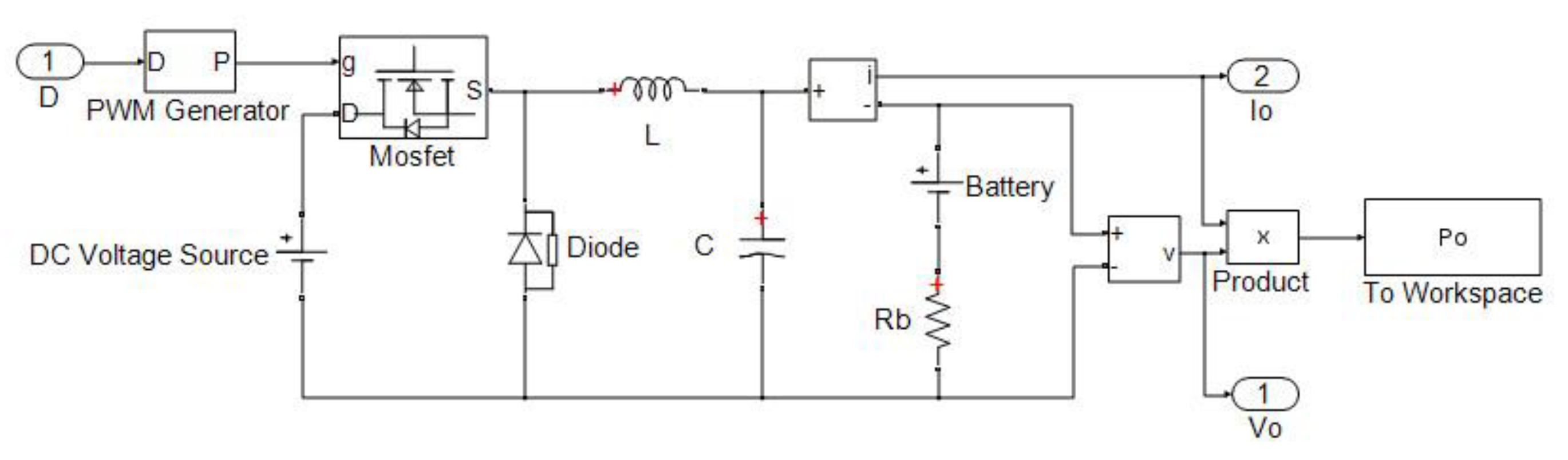
As a control device, a DC-DC Buck converter was designed, in which the output voltage Vo is controlled with a PWM signal. Figure 1 shows the design of the DC-DC Buck converter developed in MATLAB/Simulink with the SimPowerSystem toolbox.
2.3. MPPT Controller
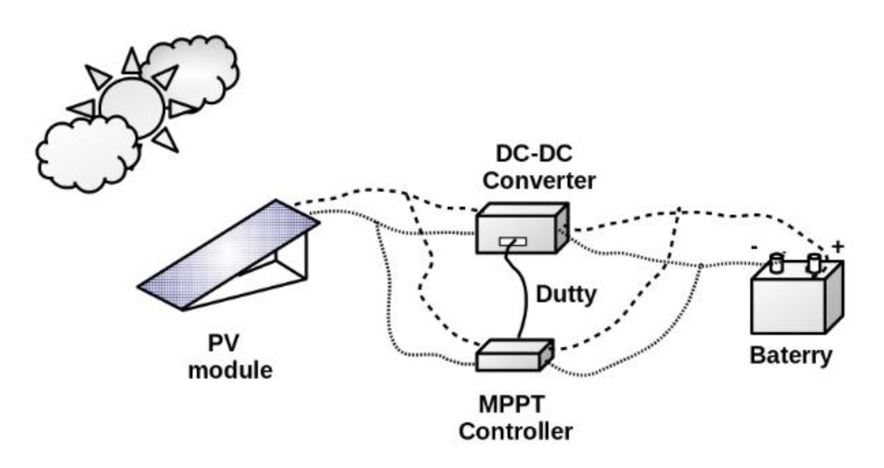
The MPPT controllers guarantee the highest available power in a PV system [30], by modifying the percentage of the duty cycle of the PWM signal, which is the input of the dc-dc converter. In this way, all the controllers were connected individually between the PV module and the dc-dc converter as shown in Figure 2.
2.3.1. P&O Algorithm
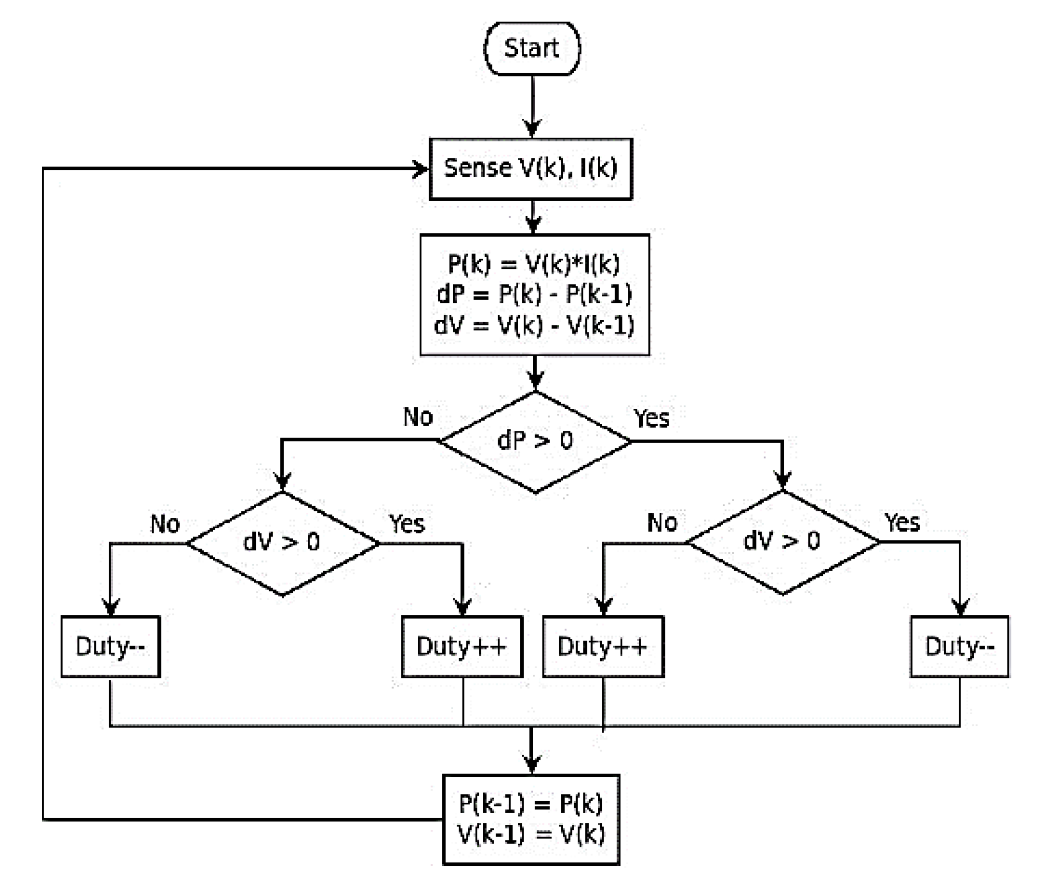
The P&O algorithm consists of performing a disturbance, modifying the voltage and observing the resulting variation in power [27]. In this algorithm, the duty cycle (D) of the DC-DC converter is adjusted depending on the value of the power change (dP). Figure 3 shows the flow diagram that was designed for this algorithm.
2.3.2. RTRL Algorithm
The intelligent control technique for the MPPT proposed in this work, is based on the design of a neural network type ADALINE, with FIR architecture, and trained with the RTRL algorithm in order to minimize the oscillations of the P&O algorithm. FIR architecture is characterized by being easy to design, configure, and implement.
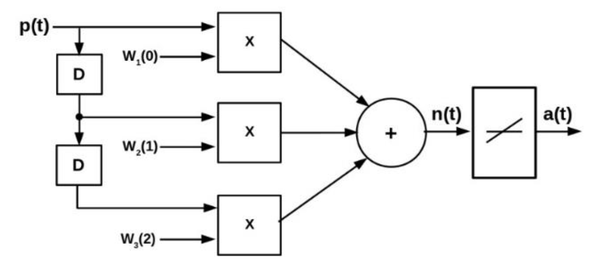
To use the ADALINE neural network as an adaptive filter, it was necessary to introduce a line of delays (D) in order to modify the impact that the synaptic weights generate on the network response. The RTRL algorithm is developed for a single neuron as can be seen in Figure 4. For the voltage and current signals that were used, it is not necessary to use the bias, since there is no displacement through the hyperplane. Equation (4) represents the output of the network.
where p(t) represents the inputs of the network over time, W is the vector of synaptic weights, a(t) is the output of the neural network, n(t) is the weighted sum of the inputs and weights before the activation function, and d indicates the delay time with respect to the first input data.
In developing Equation (4), the network response can be obtained from the first instant of time. The sum of the quadratic error F(x) represents the standard performance function that was chosen for the training. The gradient was calculated from this performance function [32]. See Equation (5).
where x is the vector that contains the parameters of the network (synaptic weights), Q is the number of samples, e2(t) is the mean square error, and t(t) are the target values of the duty cycle.
The execution of the RTRL algorithm advances very rapidly over time, since it allows simultaneous calculation of the network and the calculation of the explicit derivatives of Equation (6), which is solved with the help of the chain rule. The development of this equation has some aspects similar to the backpropagation algorithm used in static multilayer networks [32]. u is the number of layers in the network.
Finally, with the development of Equation (7) the synaptic weights obtained in the training are updated.
where α is the dynamic learning rate.
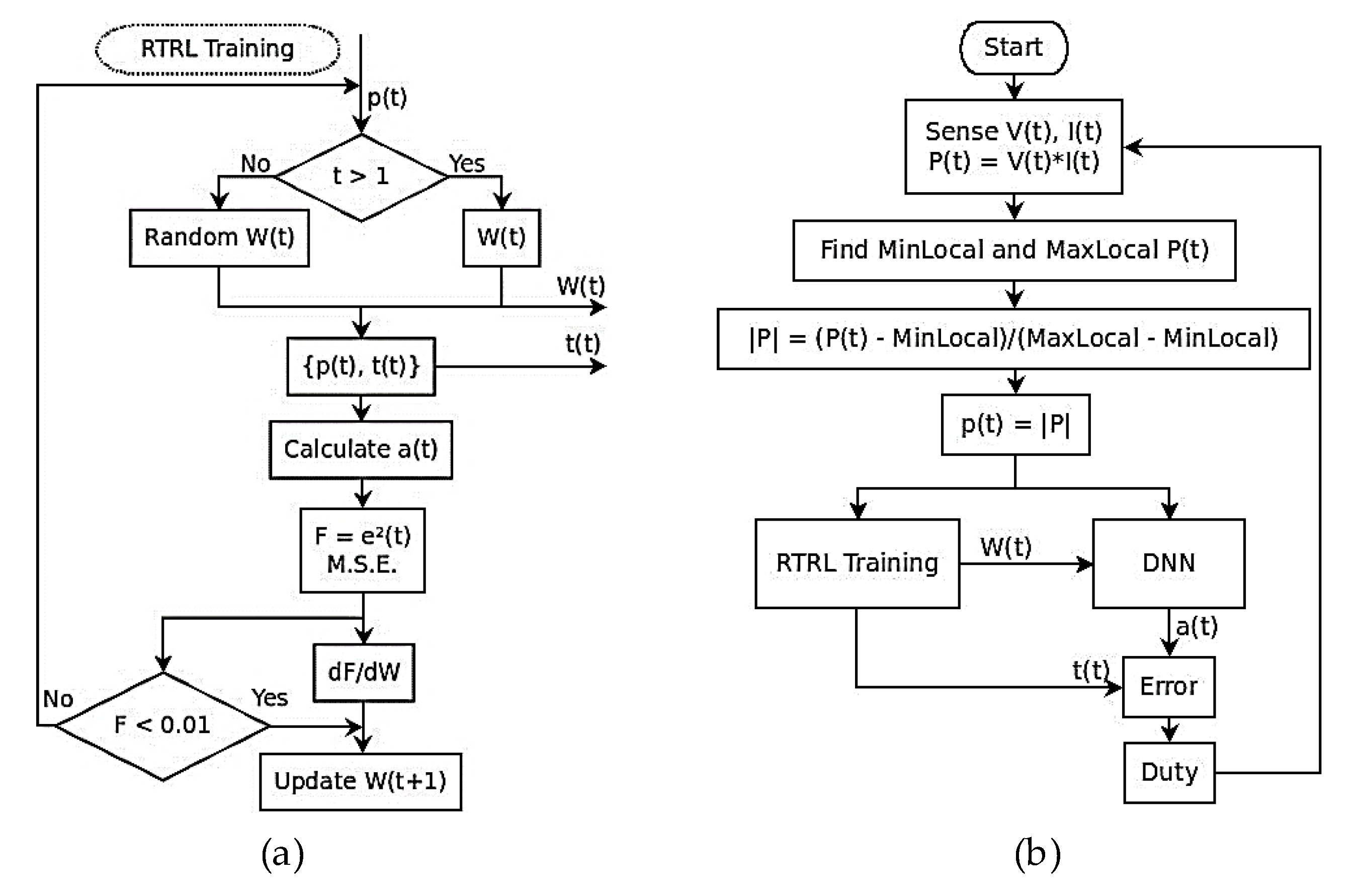
Figure 5a shows the flow diagram of the RTRL algorithm used to train the dynamic network. The behavior of the dynamic neural controller is shown in Figure 5b.
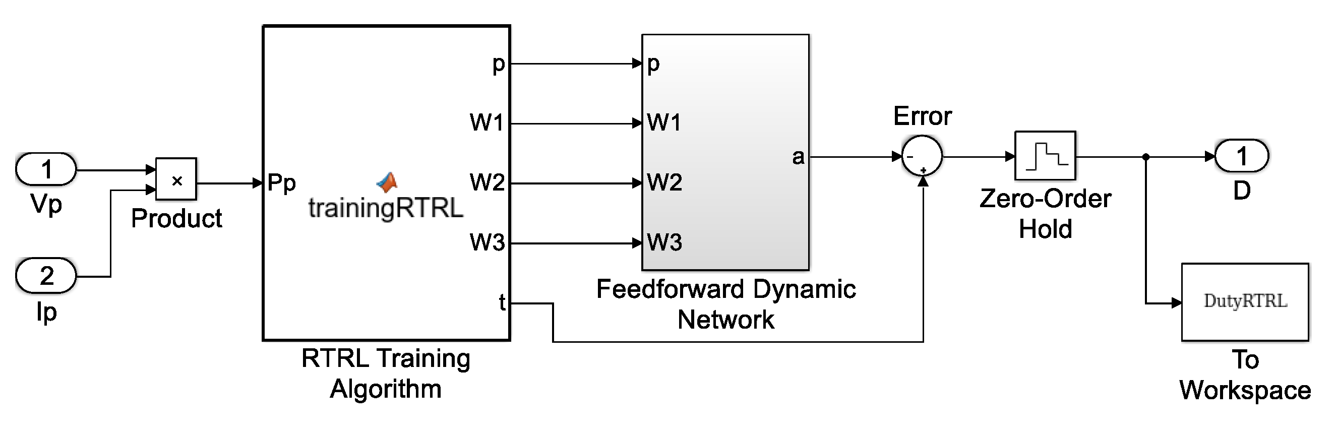
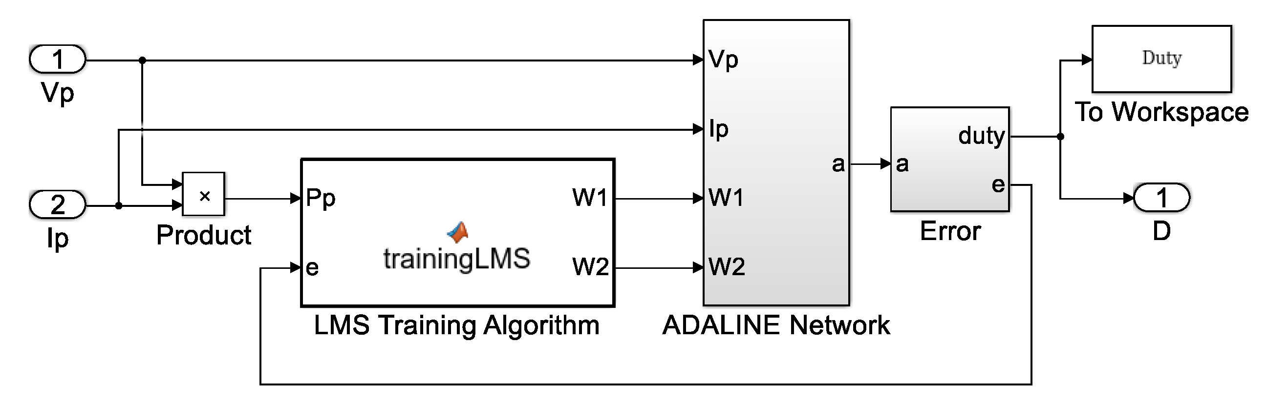
Figure 6 shows the block diagram of the RTRL neurocontroller designed in MATLAB/Simulink, in which it is emphasized that it was not necessary to use the Neural Networks Toolbox to design the control system. The block “Error” of Figure 6 is responsible for filtering the oscillations that may occur when trying to track the MPP.
2.3.3. LMS Algorithm
Widrow and Marcian Hoff developed the ADALINE neural network with their own learning algorithm (LMS: Least Mean Square) [32]. To take advantage of this learning method in digital signal processing, the two versions of the LMS algorithm (LMS and Iterative LMS) were implemented using the same network architecture.
The design of the ADALINE network with LMS algorithm consists of a vector array of input data, synaptic weights, and target, which are subsequently used in various matrix calculations. The construction of these matrices is key to determining the MSE (Mean Squared Error) and the final synaptic weights at the first instant time, since the mathematical process is performed only once. See Equations (8)–(10).
The vector Z has the input values of the network, T is the transpose of the vector, c is a constant, h is the cross-correlation between the vector of inputs and the vector associated with the input t, and R is the correlation matrix. The input vectors determine if there is a single solution of the system [32]. However, it must be verified that the array of vectors does not result in a square matrix. Therefore, for this training method the ADALINE network has only one delay.
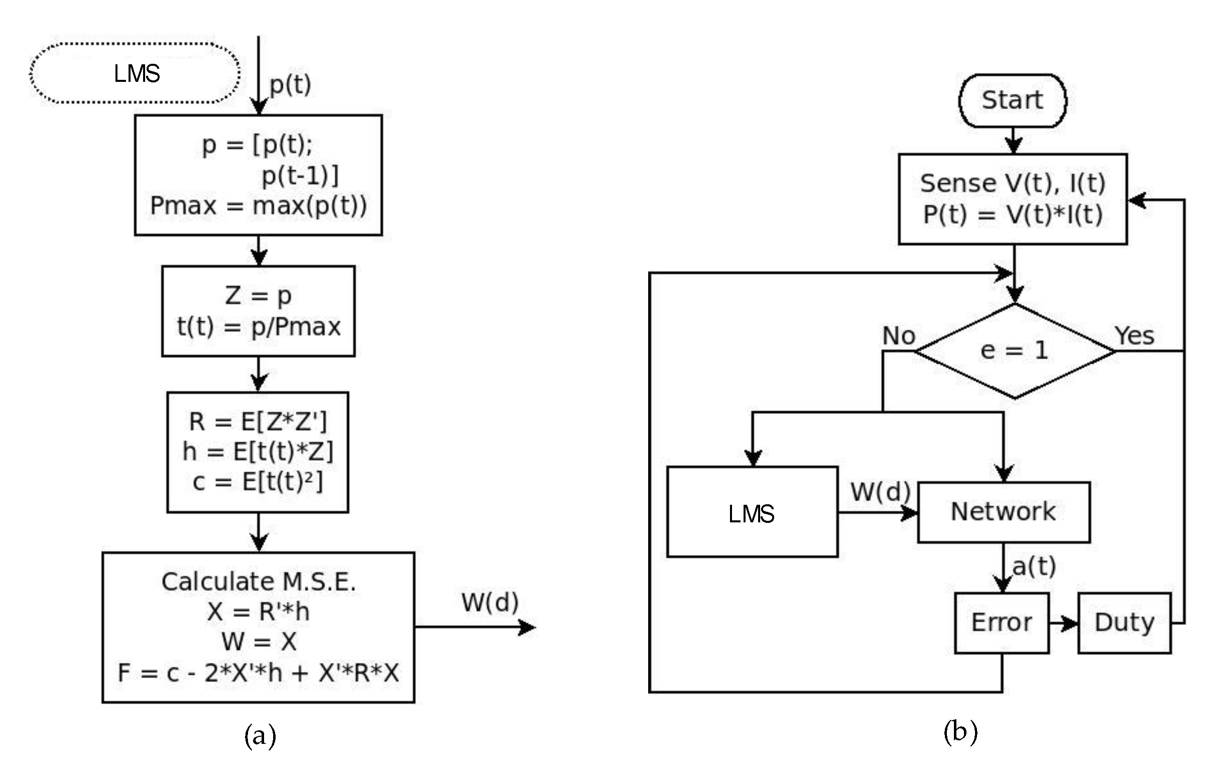
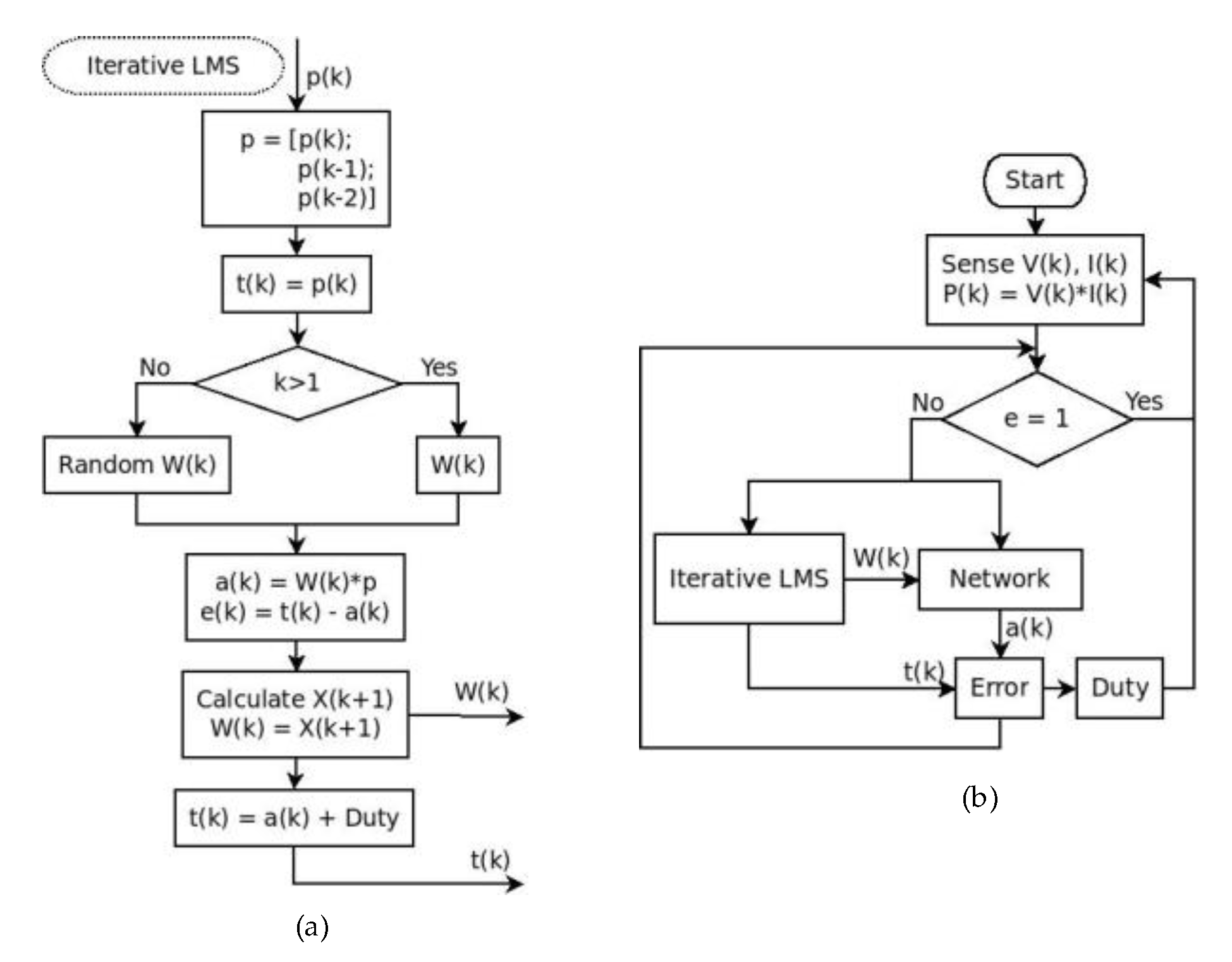
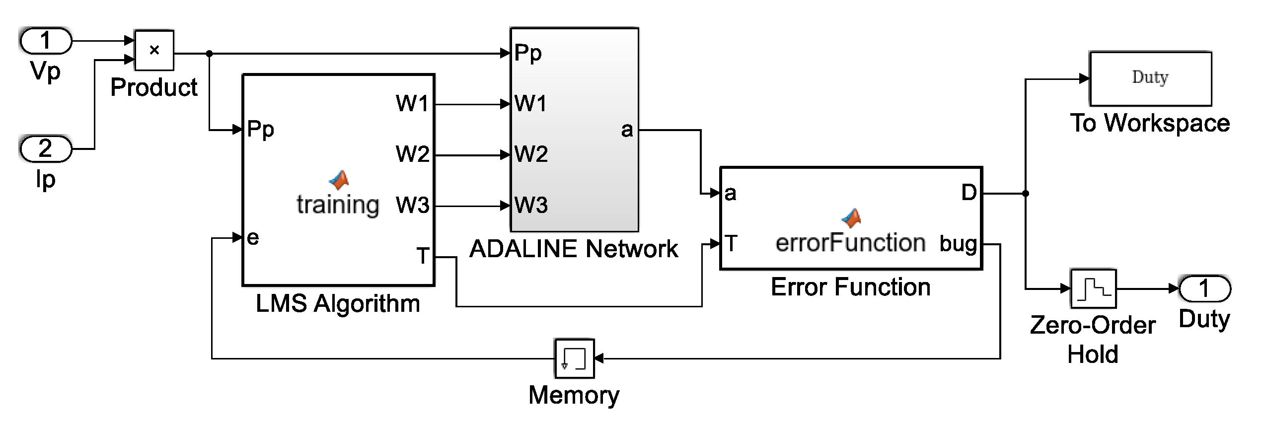
The training algorithms and the LMS controllers that were developed are shown in Figure 7 and Figure 8. In these figures it is shown that these controllers were trained with the standard procedure defined through their operating equations.
As seen in Figure 7 and Figure 8, the LMS algorithms, in their two versions, have in common the procedure used to minimize the MSE with iterations. For this, the steepest descent algorithm is used, with which the gradient can be calculated, and the performance index analyzed.
During each iteration k the synaptic weights are adjusted, and the error is obtained. This is done until the function converges. See Equation (11).
Figure 9 corresponds to the LMS subsystem and Figure 10 corresponds to the Iterative LMS subsystem, which were designed in MATLAB/Simulink. The architecture of the ADALINE neural network was built with operational blocks, such as, products, addition, and subtraction; while the training algorithms were programmed with the Simulink function blocks.
3. Results and Discussion
In order to evaluate the performance of the RTRL Neurocontroller, comparisons with the P&O and LMS algorithms were made. In addition, comparisons were established with the previous results obtained in the Magma Ingeniería research group with a fuzzy controller [12] and a controller with an NARX network [25]. Finally, a set of tables with the results of the comparisons are presented. For each control method, the maximum efficiency is calculated.
It is important to highlight that the performance of the algorithms developed in this work will be measured in terms of the power obtained by the controllers, the efficiency and the settling time. Additionally, the performance of all controllers will be evaluated according to the computation time necessary to perform the simulations.
3.1. Performance of the RTRL Neurocontroller
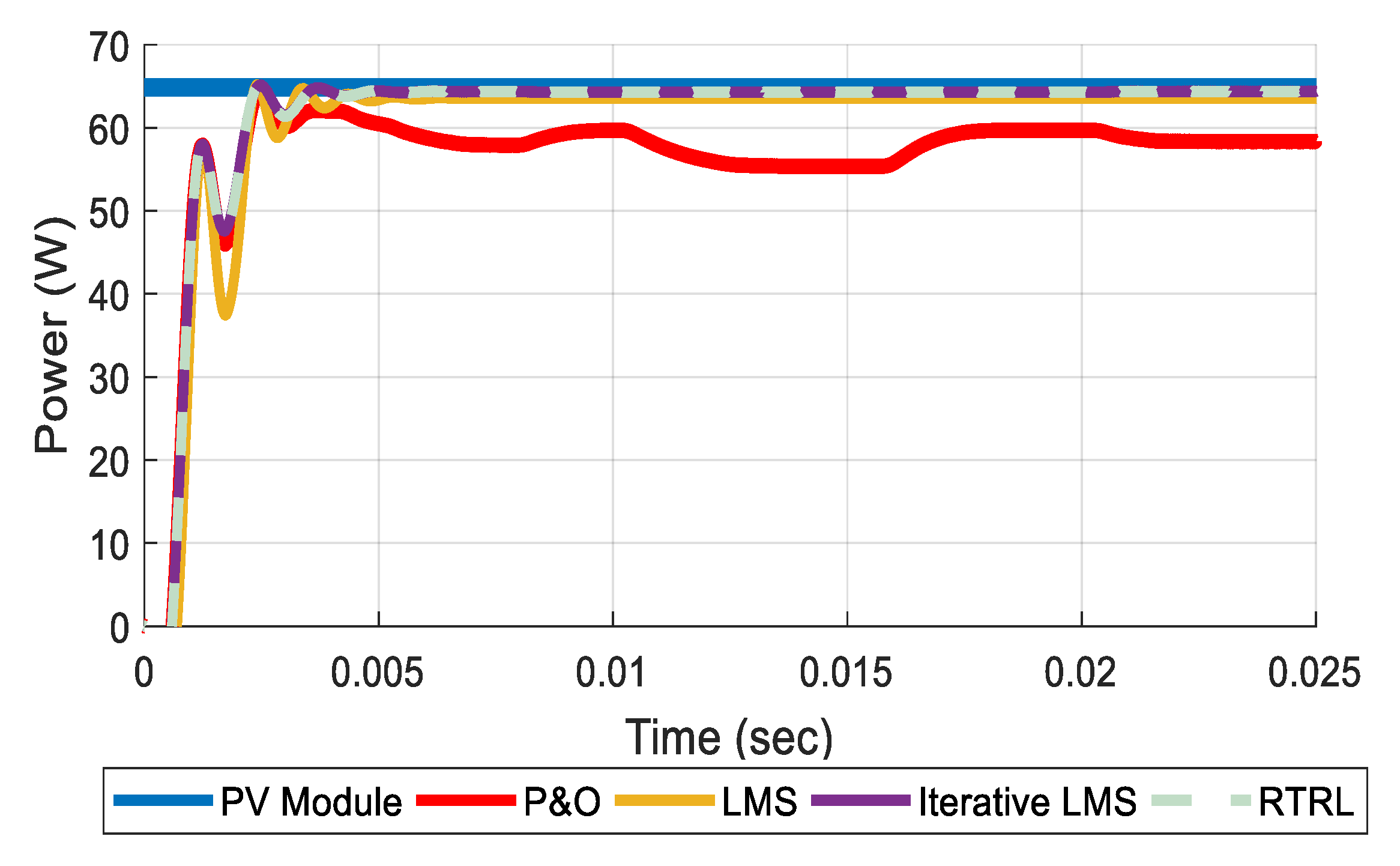
The results of the ADALINE neural network with the RTRL algorithm were compared directly with the P&O and LMS algorithms (LMS and Iterative LMS) under the same conditions of solar irradiance, temperature, and simulation time, in order to observe their responses and evaluate the performance of each of these methods. For standard test conditions with a solar irradiance of 1000 W/m2 and operating temperature of 25 °C the signals shown in Figure 11 were obtained.
In order to verify the behavior of the oscillations, the simulation time was increased to 1 s and in addition, a signal was designed to simulate the variable irradiance conditions represented by Figure 12. In Figure 13 it can be seen that, by increasing the simulation time, the oscillations continue and the P&O controller does not stabilize in the MPP.
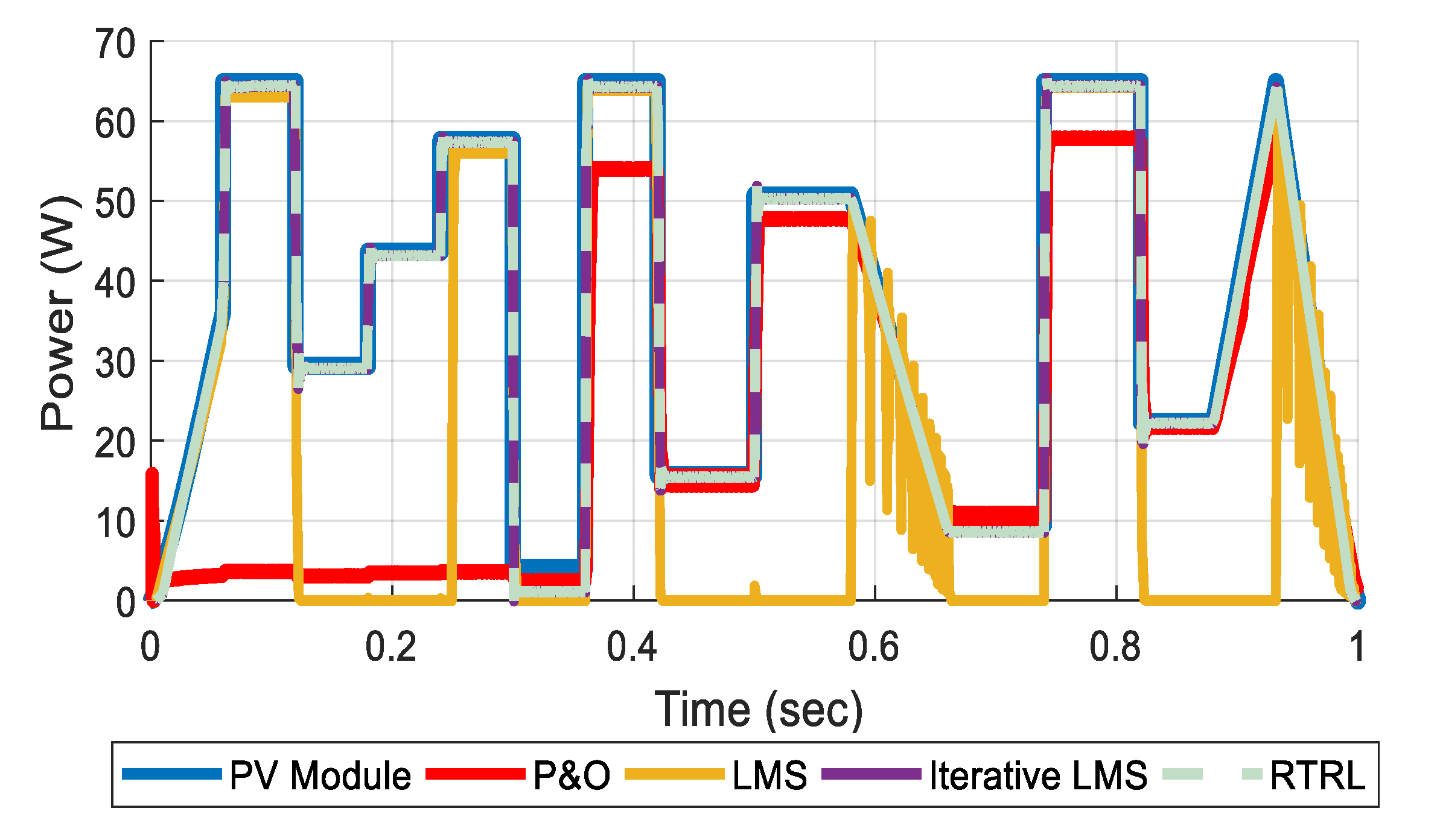
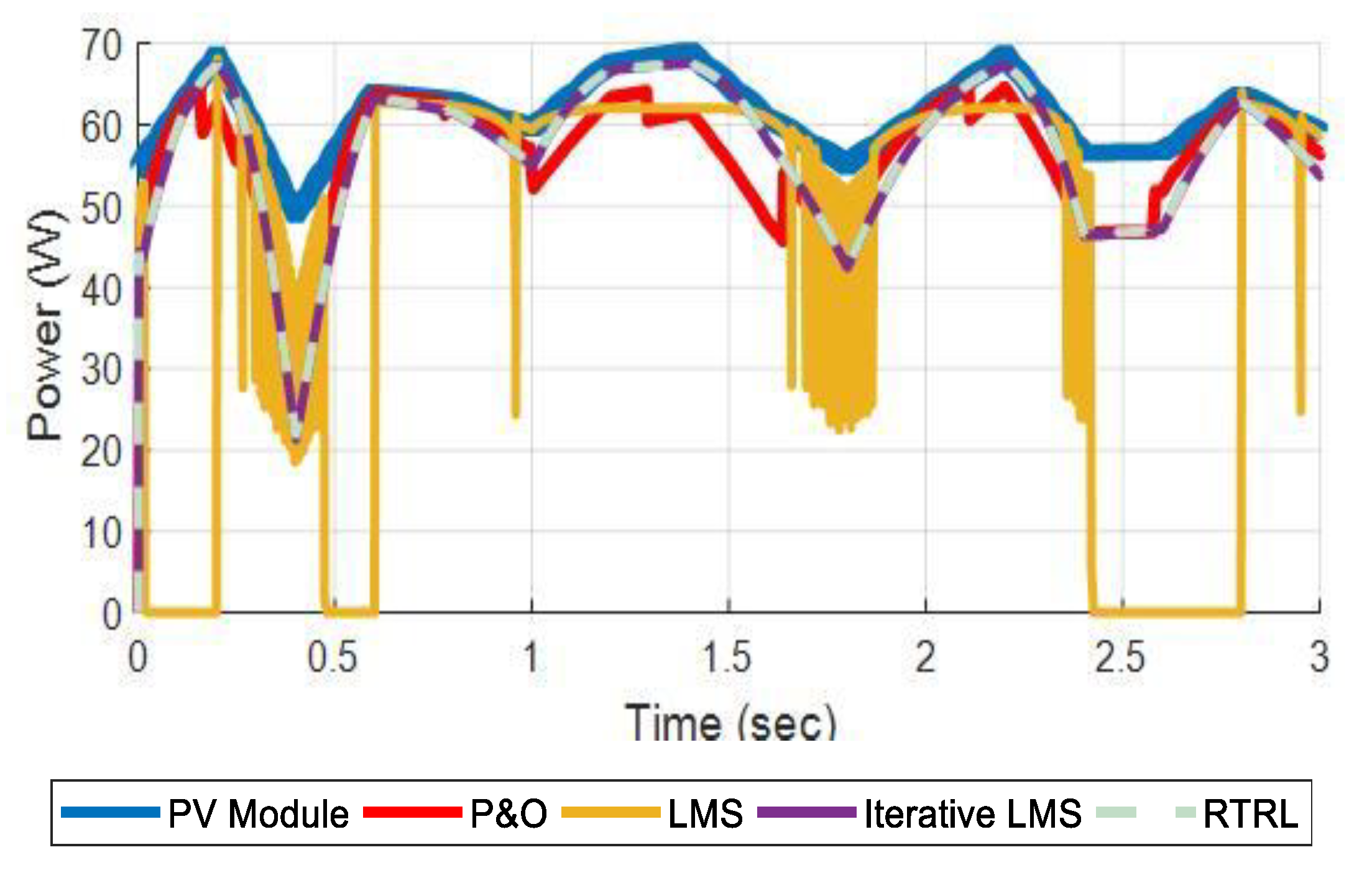
After evaluating the performance of the controllers for a variable irradiance signal, the signal of Figure 14 was designed to evaluate the performance for a variable temperature signal. The results obtained are shown in Figure 15, in which it can be noted that the P&O algorithm has oscillations throughout the simulation time. On the other hand, the LMS algorithm does not stabilize in the MPP and has oscillations of greater amplitude.
The Neurocontroller with the Iterative LMS algorithm showed good results for both irradiance and constant temperature as well as for variable conditions, and its performance was similar to that obtained with the RTRL Neurocontroller.
3.2. Comparison of the RTRL Neurocontroller with the P&O Controller
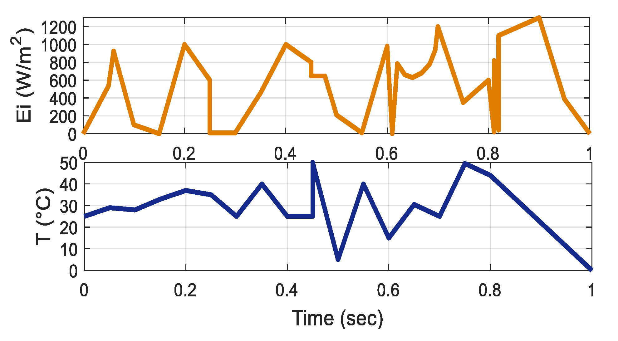
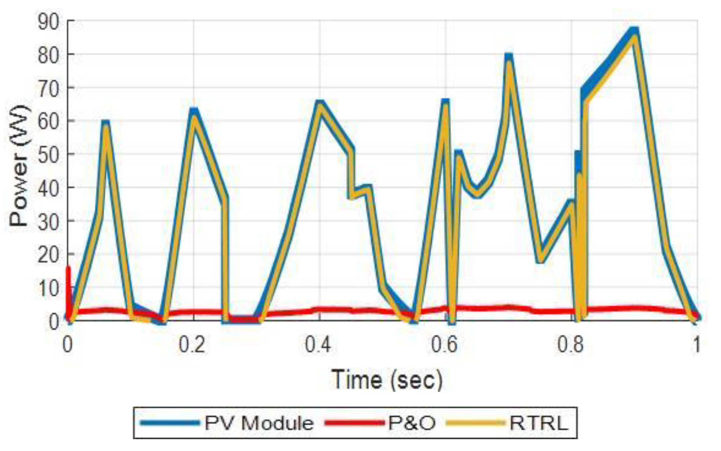
The conditions presented in Figure 16 denote a more complex scenario with sudden changes in the solar irradiance and operating temperature. The RTRL and P&O controllers were exposed to these conditions and their responses were compared simultaneously.
The results shown in Figure 17 indicate that the P&O controller has power losses when there are abrupt and proportional changes in the incident solar irradiance in the PV module.
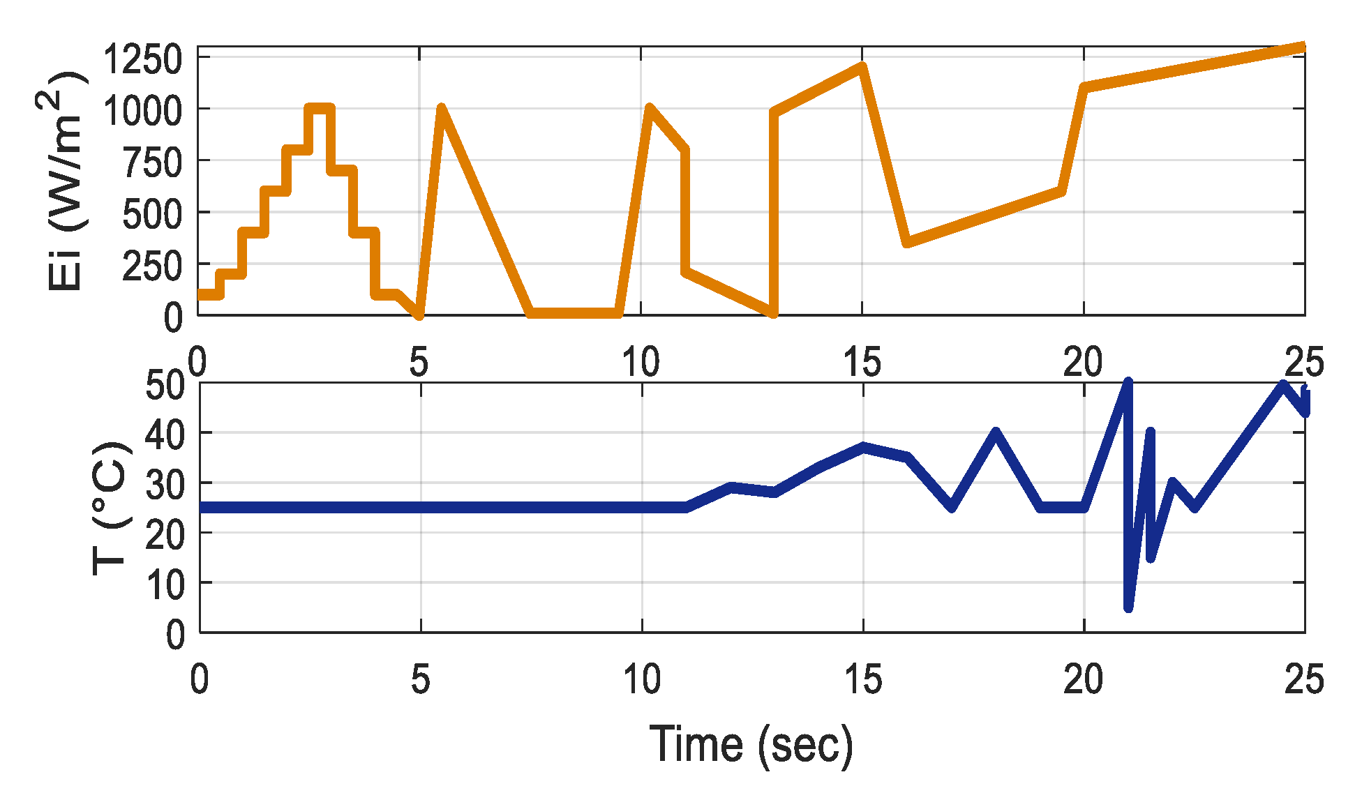
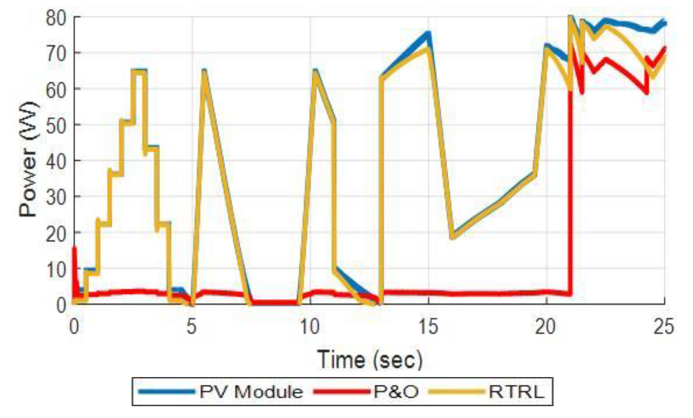
In order to evaluate the performance of the controllers for a longer simulation time, the test signal of Figure 18 was designed for a simulation time of 25 s.
Figure 19 shows the results obtained, equivalent to 6 min of computational processing. These results demonstrate the robustness of the RTRL algorithm to support sudden changes and different operating conditions in the PV module. On the other hand, the P&O algorithm improved its performance in the simulation time greater than 20 s, however, it still shows power losses.
3.3. Comparison of the RTRL Neurocontroller with the Fuzzy Controller
In this section we present the results obtained when making a comparison between the RTRL neurocontroller and the fuzzy controller developed by researchers working in the same research group as the authors of this paper. The controllers were evaluated with the same conditions of irradiance and temperature to compare their behavior and determine which has a better response. It should be noted that to carry out these tests, the authors of the fuzzy controller provided us with their modeling and simulation files.
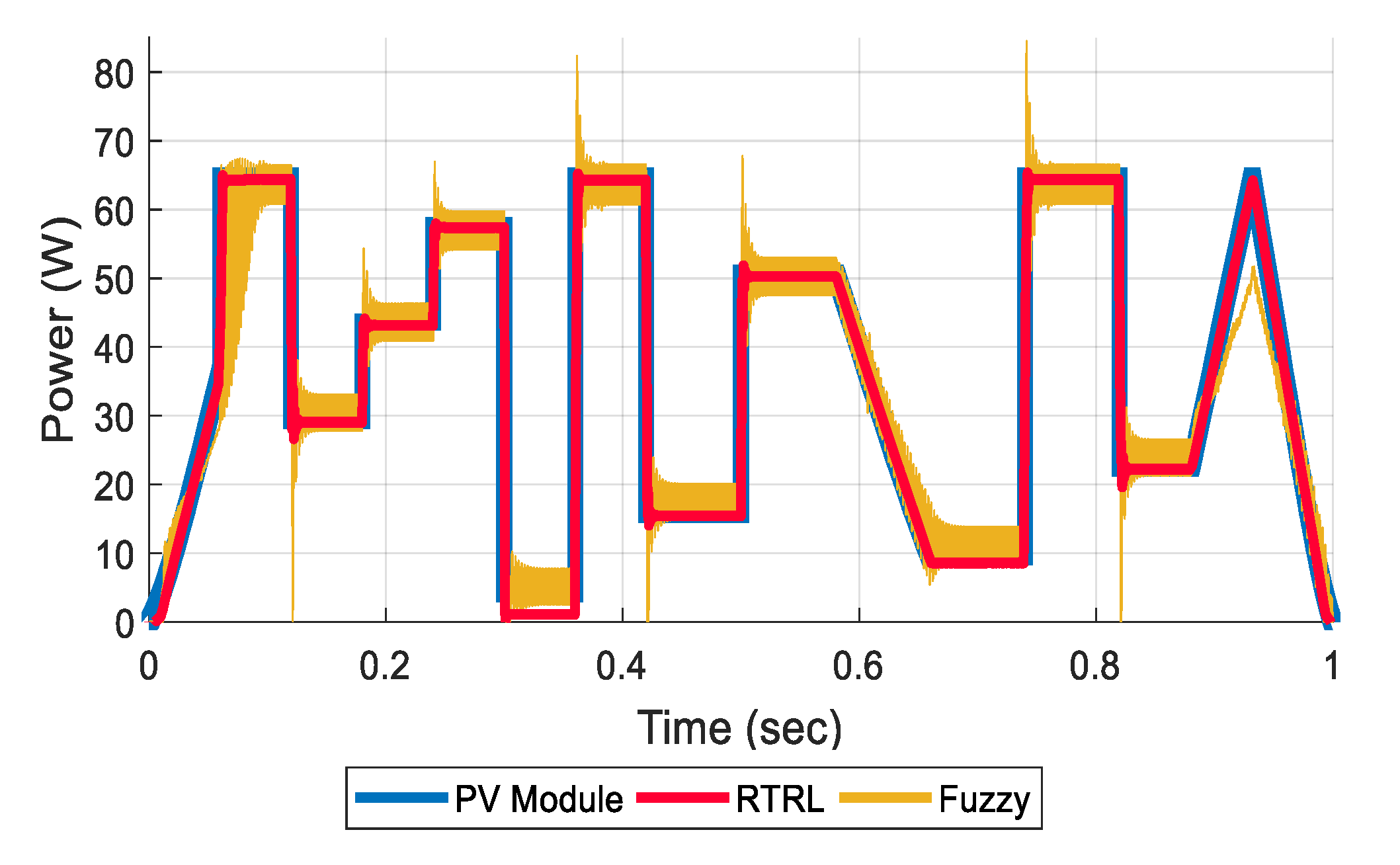
In these simulations we noticed that the fuzzy controller showed good results that can be seen in Figure 20. For a simulation time of 1 s, the fuzzy controller lasted approximately 14 min, while the RTRL for the same simulation time lasted only 19 s. For these tests, the variable irradiance signal of Figure 12 was used.
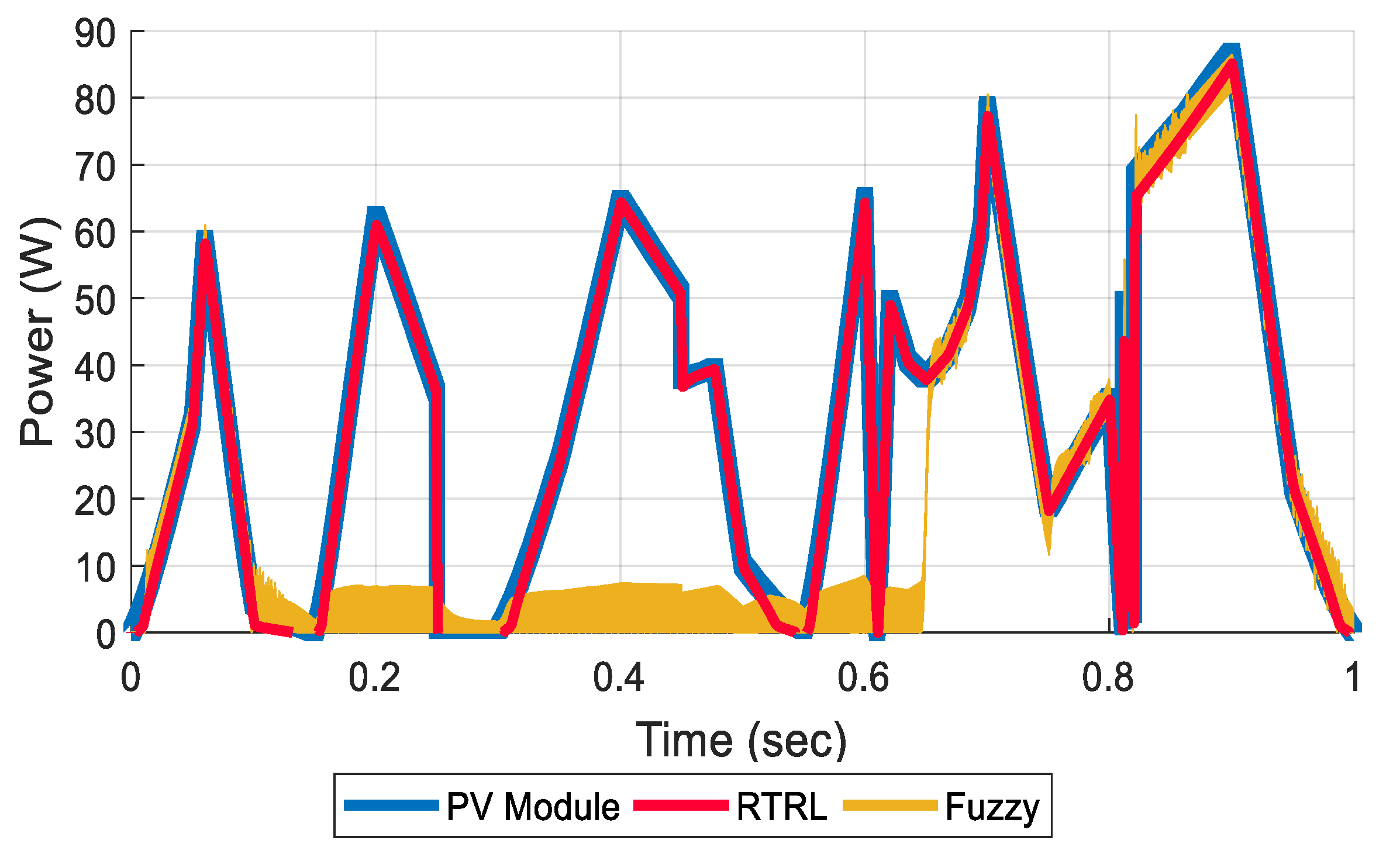
The two controllers presented a good response time, compared to the P&O algorithm, but the controller trained with the RTRL algorithm stands out for minimizing oscillations and for stabilizing faster than the fuzzy controller. In Figure 21 we note that using the irradiance and temperature signals of Figure 16, the fuzzy controller tracks the MPP during the first 0.1538 s of simulation. However, when there is a positive slope and several disturbances, the controller does not stabilize in the MPP and remains oscillating between 5 W for approximately 0.5 s of simulation. After 0.656 s, the controller responds again and tracks the MPP.
These results show that the RTRL controller has an excellent performance, since it minimizes power losses due to oscillations.
3.4. Comparison of the RTRL Neurocontroller with the NARX Neurocontroller
In this section we present the results obtained when making a comparison between the RTRL Neurocontroller and the NARX Neurocontroller [25] developed by researchers working in the same research group as the authors of this work. In [25] a neural controller of inverse model was implemented, which consists of a nonlinear autoregressive network with exogenous inputs to track the MPP of a PV module. For the design of the network, the researchers used the Backpropagation training algorithm with Levenberg-Marquardt optimization, which was designed with the MATLAB Neural Network Toolbox.
The NARX network has the same inputs (current and voltage) and the same output (duty cycle) as the RTRL neurocontroller proposed in this work. The difference between these two controllers is that the dynamic neural network with RTRL algorithm only has a neuron with Pureline activation function, whereas the NARX network has in its hidden layer 10 neurons with Tansig transfer function (Sigmoid Tangent) and a neuron in its output layer with Pureline transfer function for the duty cycle.
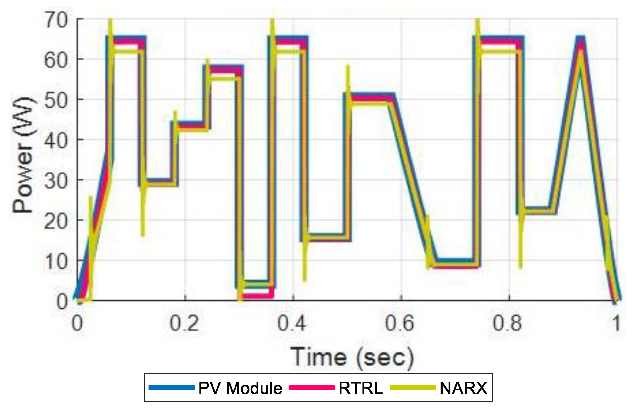
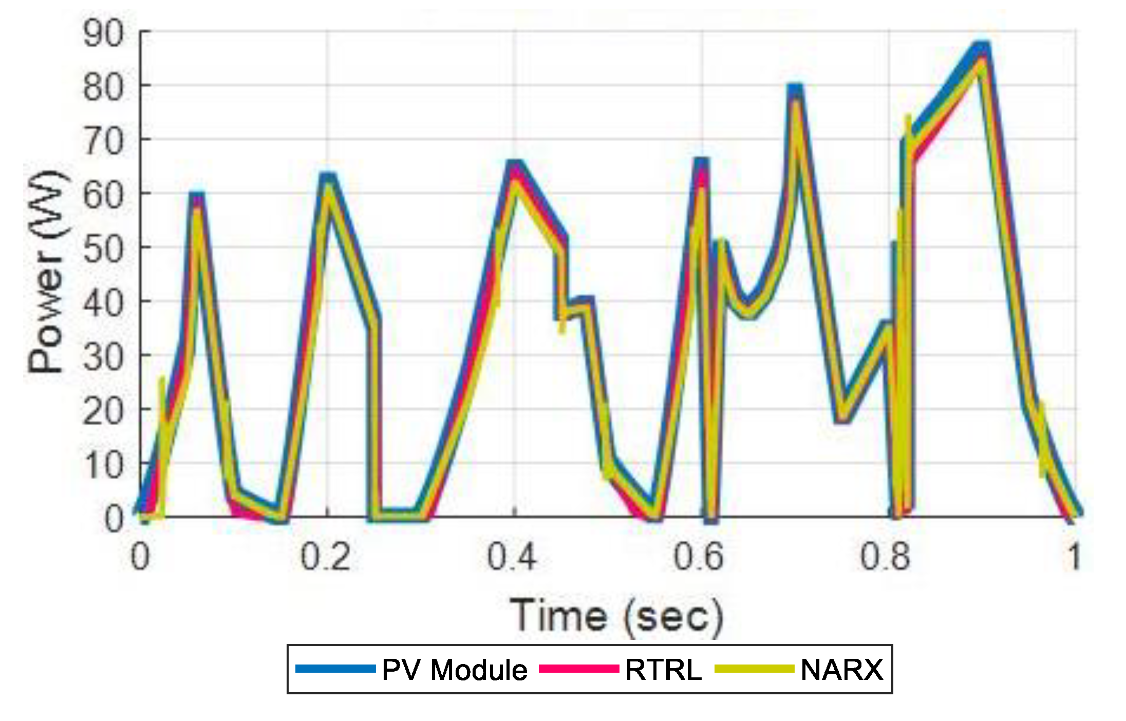
Figure 22 and Figure 23 show the results obtained with the simulations of the RTRL and NARX controllers. Both controllers track the ideal output power of the PV module and have fewer oscillations than the P&O controller. However, at each change in operating conditions, the NARX neurocontroller has strong oscillations and stabilizes after approximately 0.0325 s. In contrast, the RTRL neurocontroller stabilizes at approximately 0.005295 s and without oscillations.
It is important to note that for the simulation of 1 s, the NARX neurocontroller in the MATLAB/Simulink software lasted approximately 7 h of computational processing, while the RTRL controller for the same simulation time lasted only 22 s.
3.5. Performance of the Control Algorithms for the MPPT
In order to analyze the performance of all the control algorithms, 5 test scenarios were designed with different values for the solar irradiance and the operating temperature of the PV module (Table 1). For case 2, the average value of the solar irradiance signal of Figure 12 was used. In case 3, the average value of the temperature signal of Figure 14 was used. For cases 4 and 5, the average values of the temperature and solar irradiance signals of Figure 16 and Figure 18 were used.
Table 2 shows the maximum power values obtained during the simulation of the 5 cases, in which it can be seen that the Iterative LMS and RTRL controller showed similar power values. In each case, the power data presented for each controller represents an average value.
Generally, the controllers showed a good performance under standard test conditions (Case 1) and for conditions of variable irradiance and constant temperature (Case 2), except for the P&O algorithm that stands out for having oscillations and low efficiency. Under conditions of constant irradiance and variable temperature (Case 3) the P&O algorithm showed good results and obtained an efficiency of 91.69%, despite not tracking the MPP completely.
For the most demanding test conditions in which variable signals of irradiance and temperature were used (Cases 4 and 5), exposing the PV module to sudden changes and very steep slopes, the RTRL neurocontroller showed the maximum possible efficiency in most of the tests (See Table 3).
The efficiency (η) was found as the ratio of the average values of the power reached by each control method (Po) and the average values of the power obtained from the PV module (Pref) [38].
The results of Table 4 show the efficiency of the ADALINE network, in terms of computing time, for each of the three training algorithms (RTRL, LMS and Iterative LMS). These results are due to the fact that the ADALINE network only uses one (1) layer for its operation and that, in addition, for each algorithm only one (1) training cycle was needed.
This information is consistent with the results obtained in [39], where the performance of five training algorithms was evaluated (ADALINE, Backpropagation, Levenberg-Marquardt, Simulated Annealing, Genetic Algorithm). In this work, the authors showed that the ADALINE network showed the best performance, which was measured in terms of the number of training cycles and the MSE.
Finally, Table 5 shows the settling times, peak power, and rise time, which were obtained for a simulation time of 0.025 s, irradiance of 1000 W/m2, and temperature of 25 °C. It is highlighted that the best settling times were obtained with the three algorithms based on the ADALINE network. In this way, the efficiency of the algorithms developed in this work is also shown, in terms of the step-response for dynamic systems.
4. Conclusions
From the development of a dynamic neural controller for the tracking of the maximum power point, it can be concluded that before designing the control system, the non-linear behavior of the PV module must be taken into account and that the output signals will be a function of the climatic conditions that are used as inputs of the module. Therefore, the simulations showed the performance of the controllers under variations in the solar irradiance and operating temperature.
With the design of the ADALINE network with its different training methods, it was possible to develop different control methods to solve the problem presented by the P&O algorithm. However, it was established that only the RTRL algorithm showed an optimal response.
The mathematical development of the ADALINE network and the RTRL algorithm was a very efficient process, since only 6 previous data were used for the training. This situation contrasts with the 50.931 power data that was used in the training of the NARX controller. In addition, it was not necessary to use the MATLAB Neural Network Toolbox to perform the controller training.
Dynamic neural networks have a high computational cost compared with other neural network control systems. However, the simulations of the control methods developed in this work required much less time than the control methods used in the comparisons. The small database used for the training was the most appropriate, since a single neuron was designed. During the literature review it was possible to confirm that the other neural control methods need more than one layer and more than one neuron to obtain good results.
The results of the RTRL neurocontroller simulations showed that mathematically it is possible to correct the oscillations that occur around the MPP when the P&O algorithm is used. The RTRL neurocontroller was adapted to the climatic conditions to which the PV module was exposed and presented a rapid response and a much lower error than the other training methods.
As future work, the experimental validation of the MPPT controller proposed in this paper will be carried out. The dynamic neural network trained with the RTRL algorithm will be implemented, in order to evaluate its efficiency through different experimental tests. Among the factors that will be evaluated are the efficiency, the program memory, and the data memory required by the proposed method and the execution time in the developed hardware. So far, the ADALINE neural network and the RTRL algorithm are designed in C language in mid-range and high-end PIC (Programmable Intelligent Computer) microcontrollers.
Author Contributions
J.V.-P. performed the design and modeling of the MPPT algorithms. C.R.-A. designed the experiments and wrote the paper. D.R.-L. supported the design of the ADALINE network with the RTRL and LMS algorithms.
Funding
This research was funded by Vicerrectoría de Investigación of the Universidad del Magdalena.
Conflicts of Interest
The authors declare no conflict of interest.
References
- United Nations. Available online: https://goo.gl/8EDxDv (accessed on 11 October 2018).
- REN21-IRENA. Available online: https://goo.gl/Pc2WuA (accessed on 10 October 2018).
- Stamatescu, I.; Fagarasan, I.; Stamatescu, G.; Arghira, N.; Iliescu, S.S. Design and Implementation of a Solar Tracking Algorithm. Procedia Eng. 2014, 69, 500–507. [Google Scholar] [CrossRef]
- Vieira, R.G.; Guerra, F.K.O.M.V.; Vale, M.R.B.G.; Araújo, M.M. Comparative performance analysis between static solar panels and single-axis tracking system on a hot climate region near to the equator. Renew. Sustain. Energy Rev. 2016, 64, 672–681. [Google Scholar] [CrossRef]
- El Kadmiri, Z.; El Kadmiri, O.; Masmoudi, L.; Najib, M. A Novel Solar Tracker Based on Omnidirectional Computer Vision. J. Sol. Energy 2015, 2015, 1–6. [Google Scholar] [CrossRef] [Green Version]
- Lee, J.F.; Rahim, N.A.; Al-Turki, Y.A. Performance of Dual-Axis Solar Tracker versus Static Solar System by Segmented Clearness Index in Malaysia. Int. J. Photoenergy 2013, 2013, 1–13. [Google Scholar] [CrossRef]
- Algarín, C.R.; Castro, A.O.; Naranjo, J.C. Dual-axis solar tracker for using in photovoltaic systems. Int. J. Renew. Energy Res. 2017, 7, 137–145. [Google Scholar]
- Ahmadi, S.; Abdi, S. Application of the Hybrid Big Bang–Big Crunch algorithm for optimal sizing of a stand-alone hybrid PV/wind/battery system. Sol. Energy 2016, 134, 366–374. [Google Scholar] [CrossRef]
- Roumila, Z.; Rekioua, D.; Rekioua, T. Energy management based fuzzy logic controller of hybrid system wind/photovoltaic/diesel with storage battery. Int. J. Hydrogen Energy 2017, 42, 19525–19535. [Google Scholar] [CrossRef]
- Rezaee Jordehi, A. Maximum power point tracking in photovoltaic (PV) systems: A review of different approaches. Renew. Sustain. Energy Rev. 2016, 65, 1127–1138. [Google Scholar] [CrossRef]
- Borni, A.; Abdelkrim, T.; Bouarroudj, N.; Bouchakour, A.; Zaghba, L.; Lakhdari, A.; Zarour, L. Optimized MPPT Controllers Using GA Heating for Grid Connected Photovoltaic Systems, Comparative study. Energy Procedia 2017, 119, 278–296. [Google Scholar] [CrossRef]
- Robles Algarín, C.; Taborda Giraldo, J.; Rodríguez Álvarez, O. Fuzzy Logic Based MPPT Controller for a PV System. Energies 2017, 10, 2036. [Google Scholar] [CrossRef]
- Algarín, C.R.; Fuentes, R.L.; Castro, A.O. Implementation of a cost-effective fuzzy MPPT controller on the Arduino board. Int. J. Smart Sens. Intell. Syst. 2018, 11, 1–10. [Google Scholar] [CrossRef]
- Chen, Y.-T.; Jhang, Y.-C.; Liang, R.-H. A fuzzy-logic based auto-scaling variable step-size MPPT method for PV systems. Sol. Energy 2016, 126, 53–63. [Google Scholar] [CrossRef]
- Kwan, T.H.; Wu, X. Maximum power point tracking using a variable antecedent fuzzy logic controller. Sol. Energy 2016, 137, 189–200. [Google Scholar] [CrossRef]
- Nabipour, M.; Razaz, M.; Seifossadat, S.G.; Mortazavi, S.S. A new MPPT scheme based on a novel fuzzy approach. Renew. Sustain. Energy Rev. 2017, 74, 1147–1169. [Google Scholar] [CrossRef]
- Hassan, S.Z.; Li, H.; Kamal, T.; Arifo˘glu, U.; Mumtaz, S.; Khan, L. Neuro-Fuzzy Wavelet Based Adaptive MPPT Algorithm for Photovoltaic Systems. Energies 2017, 10, 394. [Google Scholar] [CrossRef]
- Kheldoun, A.; Bradai, R.; Boukenoui, R.; Mellit, A. A new Golden Section method-based maximum power point tracking algorithm for photovoltaic systems. Energy Convers. Manag. 2016, 111, 125–136. [Google Scholar] [CrossRef]
- Gayathri, R.; Ezhilarasi, G.A. Golden section search based maximum power point tracking strategy for a dual output DC-DC converter. Ain Shams Eng. J. 2017, in press. [Google Scholar] [CrossRef]
- Chaves, E.N.; Reis, J.H.; Coelho, E.A.A.; Freitas, L.C.G.; Júnior, J.B.V.; Freitas, L.C. Simulated Annealing-MPPT in Partially Shaded PV Systems. IEEE Lat. Am. Trans. 2016, 14, 235–241. [Google Scholar] [CrossRef]
- Benyoucef, A.S.; Chouder, A.; Kara, K.; Silvestre, S.; Sahed, O.A. Artificial bee colony based algorithm for maximum power point tracking (MPPT) for PV systems operating under partial shaded conditions. Appl. Soft Comput. 2015, 32, 38–48. [Google Scholar] [CrossRef] [Green Version]
- Pradhan, R.; Subudhi, B. Design and real-time implementation of a new auto-tuned adaptive MPPT control for a photovoltaic system. Int. J. Electr. Power 2015, 64, 792–803. [Google Scholar] [CrossRef]
- Hou, W.; Jin, J.; Zhu, C.; Li, G. A Novel Maximum Power Point Tracking Algorithm Based on Glowworm Swarm Optimization for Photovoltaic Systems. Int. J. Photoenergy 2016, 2016, 4910862. [Google Scholar] [CrossRef]
- Titri, S.; Larbes, C.; Toumi, K.Y.; Benatchba, K. A new MPPT controller based on the Ant colony optimization algorithm for Photovoltaic systems under partial shading conditions. Appl. Soft Comput. 2017, 58, 465–479. [Google Scholar] [CrossRef]
- Robles Algarín, C.; Sevilla Hernández, D.; Restrepo Leal, D. A Low-Cost Maximum Power Point Tracking System Based on Neural Network Inverse Model Controller. Electronics 2018, 7, 4. [Google Scholar] [CrossRef]
- Bouselham, L.; Hajji, M.; Hajji, B.; Bouali, H. A New MPPT-based ANN for Photovoltaic System under Partial Shading Conditions. Energy Procedia 2017, 111, 924–933. [Google Scholar] [CrossRef]
- Sahnoun, M.A.; Ugalde, H.M.R.; Carmona, J.-C.; Gomand, J. Maximum power point tracking using P&O control optimized by a neural network approach: A good compromise between accuracy and complexity. Energy Procedia 2013, 42, 650–659. [Google Scholar] [CrossRef]
- Mahjoub Essefi, R.; Souissi, M.; Abdallah, H. Maximum Power Point Tracking Control Using Neural Networks for Stand-Alone Photovoltaic Systems. Int. J. Mod. Nonlinear Theory Appl. 2014, 3, 53–65. [Google Scholar] [CrossRef]
- Kofinas, P.; Dounis, A.I.; Papadakis, G.; Assimakopoulos, M.N. An Intelligent MPPT controller based on direct neural control for partially shaded PV system. Energy Build. 2015, 90, 51–64. [Google Scholar] [CrossRef]
- Messalti, S.; Harrag, A.; Loukriz, A. A new variable step size neural networks MPPT controller: Review, simulation and hardware implementation. Renew. Sustain. Energy Rev. 2017, 68, 221–233. [Google Scholar] [CrossRef]
- Amir, A.; Amir, A.; Selvaraj, J.; Rahim, N.A. Study of the MPP tracking algorithms: Focusing the numerical method techniques. Renew. Sustain. Energy Rev. 2016, 62, 350–371. [Google Scholar] [CrossRef]
- Hagan, M.T.; Demuth, H.B.; Beale, M.H.; De Jesús, O. Neural Network Design, 2nd ed.; Oklahoma State University: Stillwater, OK, USA, 2014; pp. 14–22. [Google Scholar]
- Hen Hu, Y.; Hwang, J.-N. Handbook of Neural Network Signal Processing; CRC Press LLC: Boca Raton, FL, USA, 2002; pp. 42–45. [Google Scholar]
- Haykin, S. Neural Networks: A Comprehensive Foundation, 2nd ed.; Prentice Hall: Upper Saddle River, NJ, USA, 1998; pp. 150–155. [Google Scholar]
- Robles Algarín, C.; Rodríguez Álvarez, O.; Ospino Castro, A. Data from a photovoltaic system using fuzzy logic and the P&O algorithm under sudden changes in solar irradiance and operating temperature. Data Brief 2018, 21, 1618–1621. [Google Scholar] [CrossRef]
- Ortiz, E. Modeling and Analysis of Solar Distributed Generation. Ph.D. Thesis, Michigan State University, East Lansing, MI, USA, 2006. [Google Scholar]
- Gil, O. Modelado y Simulación de Dispositivos Fotovoltaicos. Master’s Thesis, Universidad de Puerto Rico, San Juan, Puerto Rico, 2008. [Google Scholar]
- Lin, F.L.; Ye, H.; Rashid, M. Digital Power Electronics and Applications; Elsevier: New York, NY, USA, 2005; p. 7. ISBN 0-1208-8757-6. [Google Scholar]
- Hassan, M.; Hamada, M. Performance Comparison of Feed-Forward Neural Networks Trained with Different Learning Algorithms for Recommender Systems. Computation 2017, 5, 40. [Google Scholar] [CrossRef]
Figure 1.
Electrical model of the dc-dc converter designed in MATLAB/Simulink.

Figure 2.
Components of the PV system.

Figure 3.
Flowchart of the P&O algorithm.

Figure 4.
Block diagram of the ADALINE network with FIR architecture.

Figure 5.
Flow diagrams: (a) RTRL algorithm; (b) RTRL Neurocontroller.

Figure 6.
Block diagram of the RTRL Neurocontroller designed in MATLAB/Simulink.

Figure 7.
Flow diagrams: (a) LMS Algorithm; (b) LMS Controller.

Figure 8.
Flow diagrams: (a) Iterative LMS Algorithm; (b) Iterative LMS Controller.

Figure 9.
Block diagram of the ADALINE network with LMS algorithm.

Figure 10.
Block diagram of the ADALINE network with Iterative LMS algorithm.

Figure 11.
Results of the P&O, LMS, and RTRL controllers for 1000 W/m2 and 25 °C.

Figure 12.
Variable irradiance signal used for tests.

Figure 13.
Results of the P&O, LMS, and RTRL controllers under conditions of variable irradiance and constant temperature.
Figure 13.
Results of the P&O, LMS, and RTRL controllers under conditions of variable irradiance and constant temperature.

Figure 14.
Variable temperature signal used for tests.

Figure 15.
Results of the P&O, LMS, and RTRL controllers under conditions of variable temperature and constant irradiance.
Figure 15.
Results of the P&O, LMS, and RTRL controllers under conditions of variable temperature and constant irradiance.

Figure 16.
Variable irradiance and temperature signals used to evaluate the performance of the RTRL and P&O controllers.
Figure 16.
Variable irradiance and temperature signals used to evaluate the performance of the RTRL and P&O controllers.

Figure 17.
Results obtained with the P&O and RTRL controllers for variable signals of irradiance and temperature.
Figure 17.
Results obtained with the P&O and RTRL controllers for variable signals of irradiance and temperature.

Figure 18.
Variable irradiance and temperature signals for a simulation time of 25 s.

Figure 19.
Results obtained with the P&O and RTRL controllers for variable signals of irradiance and temperature with a simulation time of 25 s.
Figure 19.
Results obtained with the P&O and RTRL controllers for variable signals of irradiance and temperature with a simulation time of 25 s.

Figure 20.
Results obtained with the RTRL and Fuzzy controllers for a signal of variable irradiance and constant temperature.
Figure 20.
Results obtained with the RTRL and Fuzzy controllers for a signal of variable irradiance and constant temperature.

Figure 21.
Results obtained with the RTRL and Fuzzy controllers for variable signals of irradiance and temperature.
Figure 21.
Results obtained with the RTRL and Fuzzy controllers for variable signals of irradiance and temperature.

Figure 22.
Results obtained with the RTRL and NARX controllers for a signal of variable irradiance and constant temperature.
Figure 22.
Results obtained with the RTRL and NARX controllers for a signal of variable irradiance and constant temperature.

Figure 23.
Results obtained with the RTRL and NARX controllers for variable signals of irradiance and temperature.
Figure 23.
Results obtained with the RTRL and NARX controllers for variable signals of irradiance and temperature.


Table 1.
Test cases to evaluate the performance of the control algorithms.
| Case | Test Signals | |
|---|---|---|
| Ei (W/m2) | T (°C) | |
| 1 | 1000 | 25 |
| 2 | 588.38 | 25 |
| 3 | 1000 | 41.79 |
| 4 | 545.12 | 28.85 |
| 5 | 631.65 | 28.95 |
Table 2.
Maximum power obtained with each control algorithm.
| Case | Pref (W) | P&O (W) | LMS (W) | Iterative LMS (W) | RTRL (W) | Fuzzy (W) | NARX (W) |
|---|---|---|---|---|---|---|---|
| 1 | 64.87 | 56.05 | 60.16 | 61.14 | 61.33 | 57.28 | 58.88 |
| 2 | 36.13 | 22.37 | 20.5 | 35.37 | 35.47 | 33.03 | 34.57 |
| 3 | 61.4 | 56.3 | 39.61 | 55.33 | 57.09 | 57.47 | |
| 4 | 33.25 | 2.79 | 28.86 | 31.96 | 32.36 | 16.87 | 31.61 |
| 5 | 38.86 | 12.84 | 36.29 | 36.43 | 37.19 | 32.54 |
Table 3.
Maximum efficiency obtained for the simulated control algorithms.
| Case | η (P&O) | η (LMS) | η (Iterative LMS) | η (RTRL) | η (Fuzzy) | η (NARX) |
|---|---|---|---|---|---|---|
| 1 | 86.4% | 92.74% | 94.25% | 94.54% | 88.3% | 90.77% |
| 2 | 61.92% | 56.74% | 97.9% | 98.17% | 91.42% | 95.68% |
| 3 | 91.69% | 64.51% | 90.11% | 92.98% | 93.6% | |
| 4 | 8.39% | 86.8% | 96.12% | 97.32% | 50.74% | 95.07% |
| 5 | 33.04% | 93.39% | 93.75% | 95.7% | 83.74% |
Table 4.
Simulation and computation times obtained for the controllers.
| Case | Simulation Time (Seconds) | MPPT Controller | Computation Time (hh:mm:ss) |
|---|---|---|---|
| 1 | 0.025 | P&O | 00:00:02 |
| LMS | 00:00:01 | ||
| Iterative LMS | 00:00:02 | ||
| RTRL | 00:00:01 | ||
| Fuzzy | 00:00:27 | ||
| NARX | 00:02:18 | ||
| 2 | 1 | P&O | 00:00:18 |
| LMS | 00:00:19 | ||
| Iterative LMS | 00:00:19 | ||
| RTRL | 00:00:21 | ||
| Fuzzy | 00:15:16 | ||
| NARX | 06:07:46 | ||
| 3 | 3 | P&O | 00:00:35 |
| LMS | 00:00:56 | ||
| Iterative LMS | 00:00:41 | ||
| RTRL | 00:00:45 | ||
| Fuzzy | 00:36:48 | ||
| NARX | |||
| 4 | 1 | P&O | 00:00:19 |
| LMS | 00:00:18 | ||
| Iterative LMS | 00:00:20 | ||
| RTRL | 00:00:22 | ||
| Fuzzy | 00:12:02 | ||
| NARX | 07:29:00 | ||
| 5 | 25 | P&O | 00:08:00 |
| LMS | 00:07:03 | ||
| Iterative LMS | 00:06:32 | ||
| RTRL | 00:07:33 | ||
| Fuzzy | 05:41:14 | ||
| NARX |
Table 5.
Step-response characteristics for a simulation time of 0.025 s.
| MPPT Controller | Rise Time (ms) | Settling Time (ms) | Peak (W) | Peak Time (ms) |
|---|---|---|---|---|
| P&O | 0.42 | 16.36 | 64.67 | 2.55 |
| LMS | 0.46 | 3.16 | 65.15 | 2.45 |
| Iterative LMS | 0.58 | 3.32 | 64.71 | 2.55 |
| RTRL | 0.59 | 3.34 | 65.17 | 2.50 |
| Fuzzy | 0.81 | 8.65 | 64.98 | 2.70 |
| NARX | 0.34 | 4.37 | 64.70 | 1.35 |
© 2018 by the authors. Licensee MDPI, Basel, Switzerland. This article is an open access article distributed under the terms and conditions of the Creative Commons Attribution (CC BY) license (http://creativecommons.org/licenses/by/4.0/).
Share and Cite
MDPI and ACS Style
Viloria-Porto, J.; Robles-Algarín, C.; Restrepo-Leal, D. A Novel Approach for an MPPT Controller Based on the ADALINE Network Trained with the RTRL Algorithm. Energies 2018, 11, 3407. https://doi.org/10.3390/en11123407
AMA Style
Viloria-Porto J, Robles-Algarín C, Restrepo-Leal D. A Novel Approach for an MPPT Controller Based on the ADALINE Network Trained with the RTRL Algorithm. Energies. 2018; 11(12):3407. https://doi.org/10.3390/en11123407
Chicago/Turabian StyleViloria-Porto, Julie, Carlos Robles-Algarín, and Diego Restrepo-Leal. 2018. "A Novel Approach for an MPPT Controller Based on the ADALINE Network Trained with the RTRL Algorithm" Energies 11, no. 12: 3407. https://doi.org/10.3390/en11123407
Note that from the first issue of 2016, this journal uses article numbers instead of page numbers. See further details here.