The Effect of Price-Dependent Demand on the Sustainable Electrical Energy Supply Chain


Department of Industrial and Systems Engineering, Chung Yuan Christian University, Taoyuan 32023, Taiwan
*
Author to whom correspondence should be addressed.
Energies 2018, 11(7), 1645; https://doi.org/10.3390/en11071645
Submission received: 22 May 2018
/
Revised: 14 June 2018
/
Accepted: 20 June 2018
/
Published: 24 June 2018
Abstract
:In order to identify the optimal structure of an electricity power network under the main assumption of a price dependent demand of electrical energy, we presented an optimization model that aims at analyzing the effect of price-dependent demand on the sustainable electrical supply chain system (SESCS). The system included a power generation system, transmission and distribution substations, and many customers. The electrical energy was generated and transmitted through multiple substations to our customers, and the demand for electricity by the customers is dependent on the price of electricity. In the study, we considered the transmission and the distribution costs which depend on the capacities of power generation, transmission rates and distances between stations. We utilized the inventory theory to develop our model and proposed a procedure to derive an optimal solution for this problem. Finally, numerical examples and sensitivity analysis are provided to illustrate our study and consolidate managerial insights.
1. Introduction
In recent years, the consumption of electricity has increased rapidly. Total electricity consumption in the U.S. in 2015 was more than13 times greater than in 1950 [1]. According to the electricity consumption for residential, commercial, transportation and industrial sectors has been increasing since 2015. At the end of 2018, an upsurge in the residential electricity use is predicted to occur at a rate of 100 million kWh/day, due mainly to the need for air-conditioning in homes due to increasing climate change.
The variations in electricity price can influenced the demand for electricity. The prices of electricity are set to reduce the variations in demand. Therefore, it is usually highest in the summer when total demand is high (at peak hours). In general, prices are usually higher for residential and commercial customers because it costs more to distribute electricity to them. The electricity price for industrial use is usually cheaper due to government regulation and the economics of scales [1]. With the projected consumptiongrowth and the variations in the price of electricity, our research is to provide insight to government and practitioner in their energy policy.
Banbury [2] was the first to study the electricity supply chain. A literature survey on electricity market models has been done by [3]. The model to predict electricity consumption has been developed by [4]. The electricity prices and expansion planning of power capacity has been optimized by using a stochastic programming by [5]. Genoese and Genoese [6] developed a model to measure of energy storage by applying the agent-based simulation. Pavković et al. [7] investigated the impact of high-speed wind energy for optimizing electrical energy storage systems. A mathematical model to find the break-even point of increasing electrical power capacity and electricity supply uncertainty has been presented by [8]. Fossati et al. [9] proposed a genetic algorithm to minimize cost and optimize energy in micro-grid systems. Luo et al. [10] classified the electrical energy storage technologies into six forms of stored energy. The first study using a simple inventory model to analyze the electrical supply chain was conducted by [11,12]. Taylor et al. [13] used a two-stage game theory model to study price and capacity competition in electricity market. Wu et al. [14] derived a model tostudy the conventional generation with intermittent supply. Ouedraogo [15] developed an electricity supply-demand model for the African power systems. Wangsa and Wee [16] developed the electrical supply chain using inventory theory and considering the blackout cost.
Goyal [17] focused on the integrated vendor-buyer inventory under a constant demand rate. Later, other researchers, such as [18,19,20,21,22,23] continued his work. The integrated model considering lead time and demand uncertainties have been developed by [24,25,26,27].
In reality, pricing is a marketing strategy to control the buying behavior of customers. Pricing mechanisms, such as promotions, can be employed to induce customers to buy more products. However, increasing price may result in reduced demand and consumption; this is also true in the consumption of electricity.
The purpose of our study is to analyze the effect of price-dependent demand on the sustainable electrical supply chain system (SESCS). The power is transmitted through distribution networks to multiple customers whose demands are influenced by the price of electricity. We propose a procedure to find an optimal solution. The remainder of the paper is organized as follows: in Section 2, we describe the analogyand problem of SESCS. In Section 3 and Section 4, we present the development of the mathematical model. A numerical example and sensitivity analysis are discussed in Section 5 and Section 6, respectively. Section 7 concludes the work by providing insights, managerial implications and directions for future research.
2. Analogies between Sustainable Electrical Supply Chain System (SESCS) and Supply Chain Inventory System (SCIS)
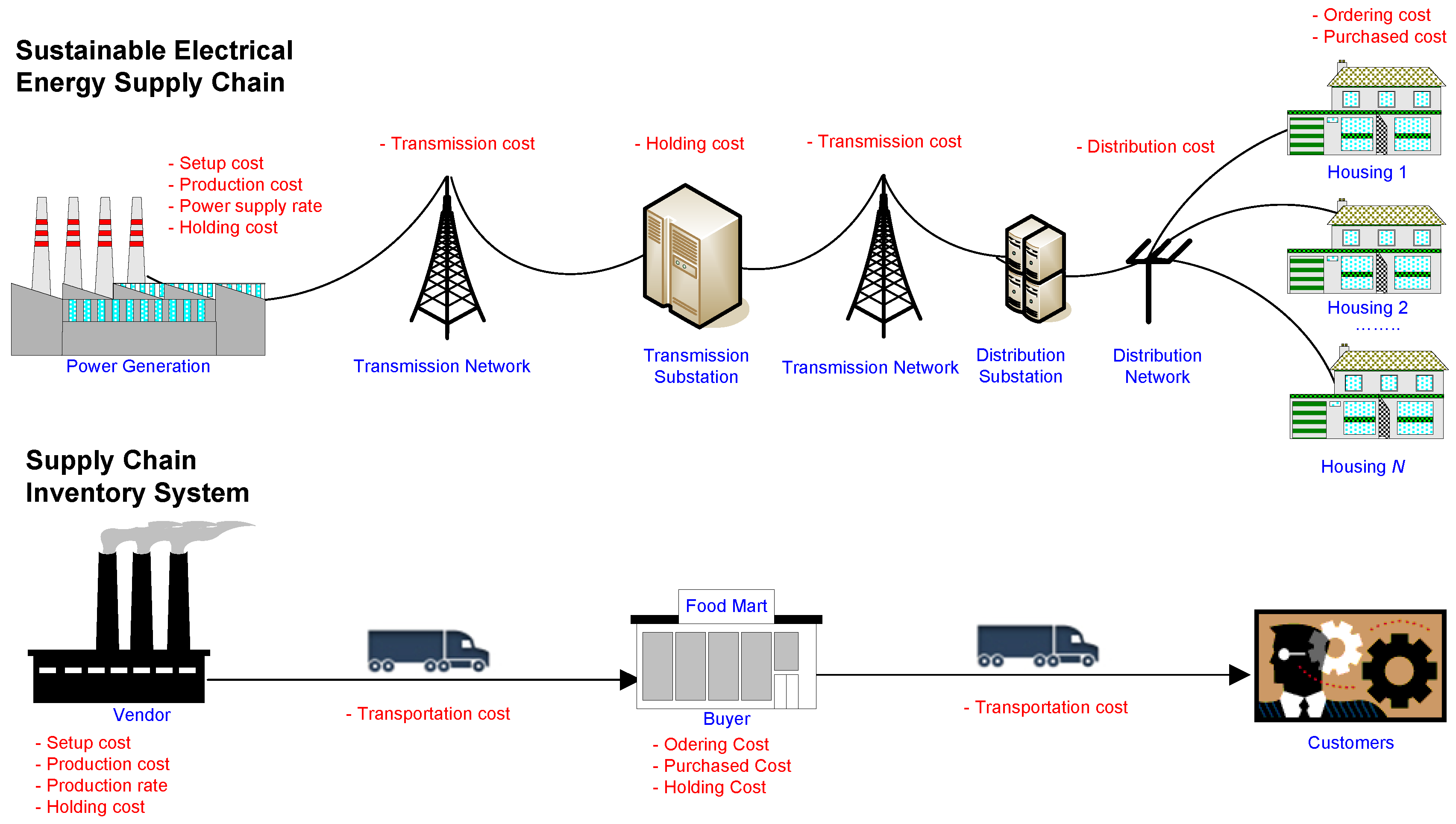
In this section, we explain the problem description of SESCS with price-dependent demand. In this study, it is shown that determining the capacity of SESCS has the same process or analogy as determining the order quantity in the Supply Chain Inventory System (SCIS). The SCIS involves a vendor-buyer coordination and freight forwarding [27]. The buyer sells items to the end-customers and orders items to the vendor. The vendor produces the items and sends in batch to the buyer. The buyer will then sell the items to the customers.
Similarly, in SESCS, electricity generated in a power generation will be transmitted through a transmission line and distribution substation to the customers whose demands are influenced by the price of electricity. The electricity demand is represented as kWh per year. The power generation produces the electricity in a batch size of kWh where m is power generation’s factor, n is transmission factor’s impact on the transmission substation and g is distribution factor’s effect on the distribution substation (integer). The finite power supply rate is P kWh per year, and a fixed setup cost of . The electricity energy of kWh is supplied by the power generator to the transmission substation, then kWh of electricity is supplied to the distribution substation and kWh of electricityis consumed by the customers.
In order to maximize the profit of SESCS, we consider the sales revenue, production cost, setup cost of the power generation, ordering cost of customers and transmission/distribution costs of substations. The transmission and distribution costs are function of the power plant, the transmission substation and the distribution substation with maximum capacities of , respectively.
The analogies between SESCS and SCIS are depicted in Figure 1.
3. Assumptions
We utilized some notations in the development of the mathematical model (see Abbreviations) and utilized the following assumptions in our model:
- The model consists of power generation, transmission and distribution substations as wellas multiple customers.
- Power supply blackouts do not occur.
- The demand rate of the customers depends on the selling price.
- We included the four types of demand rate functions:where, β > 0 is a scaling factor, and is a price elasticity coefficient.
- The finite power supply rate P is higher than the demand rate of the customers, .
- The power consumption is the sum of the electricity consumed by customers from ith to Nth, . The electricity consumption for customer ith should be in proportion to his or her electrical demand. There are .
- The electrical energy in kWh is the percentage of electricity used within a particular unit of time by customers.
- The amount of electricity energy: at generation is kWh; atthe transmission substation is kWh, at the distribution substation is kWh, and the customers consumed energy is kWh.
- The maximum capacity of power generation must be greater than at the transmission and distribution substations in KVA.
- The power generation process will include the transmission and distribution costs.
4. Mathematical Model
In this section, we explain how we first derived the total cost function with regard to customers, the distribution and transmission substations, and the total profit function of power generation.
4.1. The Customer’s Ordering Cost
Ordering cost is defined as the customer’s total cost per unit time:
4.2. The Distribution Cost
We utilized the same methodology as [16,27,28,29] to determine the distribution cost, which is incurred by the distribution substation. The distribution cost for partial load F based on the adjusted inverse function can be calculated using the equation below:
where α is the coefficient of the adjusted inverse function (0–1); its function is to increase the transmission rate per kVA per mile as the increases. The distribution cost per kVA per mile is as follows:
By combining Equation (2) into Equation (3) and simplifying, we can determine the unit rate:
The estimated total cost for the distribution substation as a function of demand, correction factor and distance with adjusted inverse yields is shown in the equation below:
The actual power supply capacity is presented as . Therefore, the distribution cost can be expressed in the following equation:
4.3. Total Cost Incurred by the Transmission Substation
This total cost consists of the energy holding cost and transmission cost. We calculated the average of these two elements using the equation below:
where, , the energy holding cost at the transmission substation is represented below:
We used the same methodology to determine the percentage of the transmission cost of distribution (Equation (6)), which can be calculated using the equation below:
Thus, the total cost incurred at the transmission substation is the sum of Equations (8) and (9). Therefore, we calculated the total cost of the transmission substation using the following equation:
4.4. Total Profit of Power Generation
The total profit of power generation can be presented by the expression:
Total profit = sales revenue − production cost − setup cost − holding cost − transmission cost.
The electricity sales revenue and production cost are given in the following equation:
Power generation creates electrical energy in kWh in one production run. Therefore, we determine the setup cost for power generation using the equation below:
The electrical energy, , the production energy , and the transmission station receive the electricity in m times of . The average energy holding for the generation of power can be evaluated as follows:
Equation (13) can be rewritten as:
Hence, the power generation’s energy holding cost is determined via the following equation:
Similar to the previous transmission cost, the production energy can be calculated via the capacity of power generation , and network from the power generation to the transmission substation . Thus, the transmission cost can be calculated as follows:
Hence, the total profit for power generation can be expressed by:
The joint total profit is the total profit of power generation and the total cost incurred by the customers, the distribution substation, and the transmission substation, which is illustrated below:
The following is a simplified version of the equation above:
Therefore, Equation (19) can be rewritten as follows:
We examined the effect of on on fixed Π(Q) by employing the first and the second partial derivatives of Equation (24) with respect to :
and:
For the fixed-integers , the function of Π(Q,g,n,m) is a concave function of . Hence, the maximum value of Π(Q,g,n,m) is located at point which satisfies . To calculate the optimal solution for fixed-integers , we utilized the partial derivatives with respect to , as shown in the following equation:
In the equation below, we set Equation (31) equal to zero and solved for, .
4.5. Procedure
In order to obtain the optimal solution values for the proposed model, we established the procedure below:
- Step 1
- We set m = 1.
- We set n = 1.
- We set g = 1.
- Step 2
- We calculated the optimal Q* by using Equation (32).
- Step 3
- Next, we calculated the actual electrical power capacities.
- Distribution Substation
- (a.1)
- We determined the actual capacity of the distribution substation via . We checked, if was satisfied. Then we revised the power consumption (Step a.2). Otherwise, , we went on to Step (b.1).
- (a.2)
- We revised the power consumption and followed Step (b.1).
- Transmission Substation
- (b.1)
- To obtain the actual capacity of the transmission substation, we utilized . We then checked if was satisfied and revised the power consumption (Step b.2). If it was not satisfied, we followed Step (c.1).
- (b.2)
- We revised the power consumption and proceeded to Step (c.1).
- Power Generation
- (c.1)
- We determined that the actual capacity of the transmission substation could be calculated via . We checked, if was satisfied, revised the power consumption (Step c.2) and proceeded to Step (4).
- (c.2)
- We revised the power consumption and moved on to Step (4).
- Step 4
- We computed Π(Q,g,n,m) using Equation (24).
- Step 5
- We set g = g + 1 and repeated Steps (2 to 4).
- Step 6
- If then we went to Step (5). If it was equal, we moved on to Step (7).
- Step 7
- We set n = n + 1 and repeated Steps (1c to 6).
- Step 8
- If we went on to Step (7). If they were equal, we moved to Step (9).
- Step 9
- Step 9 We set m = m + 1 and repeated Steps (1b to 8).
- Step 10
- If , we moved on to Step (9), otherwise we went to Step (11).
- Step 11
- We set , then were the optimal solution.
5. Numerical Example
In this example, we utilized artificial data to demonstrate the application of the model. The data values are given in Table 1, Table 2 and Table 3.
Using the mathematical model developed in previous section, we solved for the parameters given above. Table 4 shows the details of the procedure for obtaining the optimal solution. The optimal values are as follows: the customer power consumption, Q* = 350 kW or 350,000 Watt; the electrical power factors of the distribution, the transmission and the power generation are 1, 2 and 7 times, respectively. Thus, the total profit is $17,712.07/year.
In our solution (Table 5), we have m = 7 batches. It means the electricity produce by the power generatorhas a total power of 117,600.00 kWh. But not all the electricity (117,600.00 kWh) generated is transmitted at once, butin 7 times with 16,800.00 kWh each. Since the generator has a device to minimize the holding cost (Equation (15)) of the electricity, for each batch, the transmission substation receives 16,800.00 kWh of electricity; it then transmits in two batches to the distribution station at 8400 kWh each. This is done to minimize the transmission cost (Equation (9)) and distribution cost (Equation (6)).
Based on those results, the electrical power consumption of customers 1, 2, 3 and 4 are 87,507.87 Watt; 87,511.37 Watt; 87,510.49 Watt; and 87,470.26 Watt, respectively. The demand of customers 1, 2, 3 and 4 are 30,006 kWh/year; 30,007.2 kWh/year; 30,006.9 kWh/year; and 29,993.1 kWh/year, respectively. The results are shown in Table 5.
6. Discussion
In this section, we discuss the effect of changes in the parameters as well as summarize the results of the sensitivity analysis.
6.1. Price Elasticity Coefficient (γ)
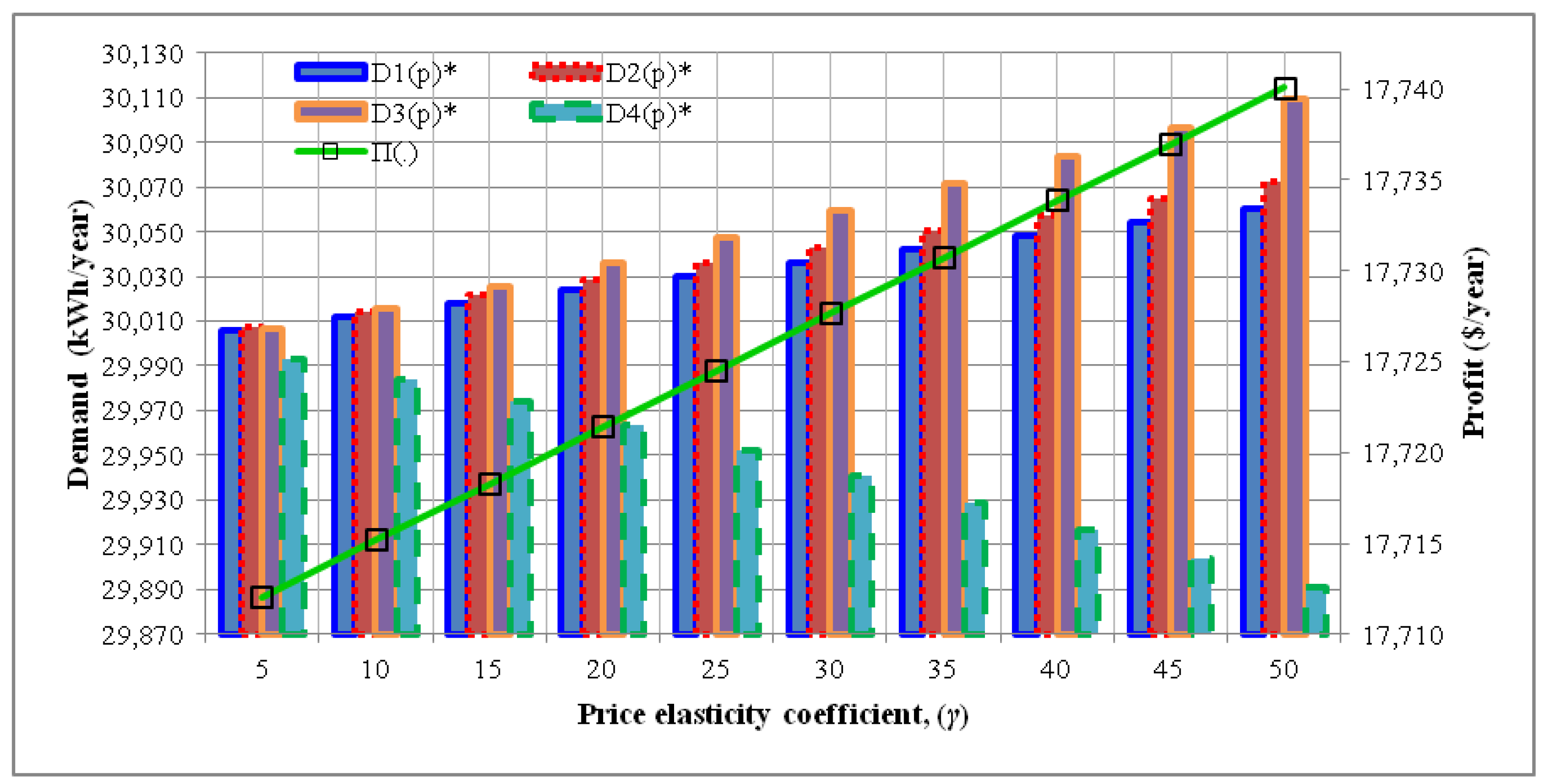
In the equation discussed above, we set the price elasticity coefficient (γ) to 5. Here, we discuss the effect of changing this coefficient from 5 to 50. Table 6 and Figure 2 show that if the price elasticity increases, then the total profit increases by an average of 0.02%. Table 6 shows an increase in the demand for customers 1, 2 and 3 and contrasts these results with customer 4′s demand. We set the demand function for customer 4 as decreasing. In many practical situations, the price elasticity can be a result of advertising that allows marketers to achieve higher profits.
6.2. Scaling Factor (β)
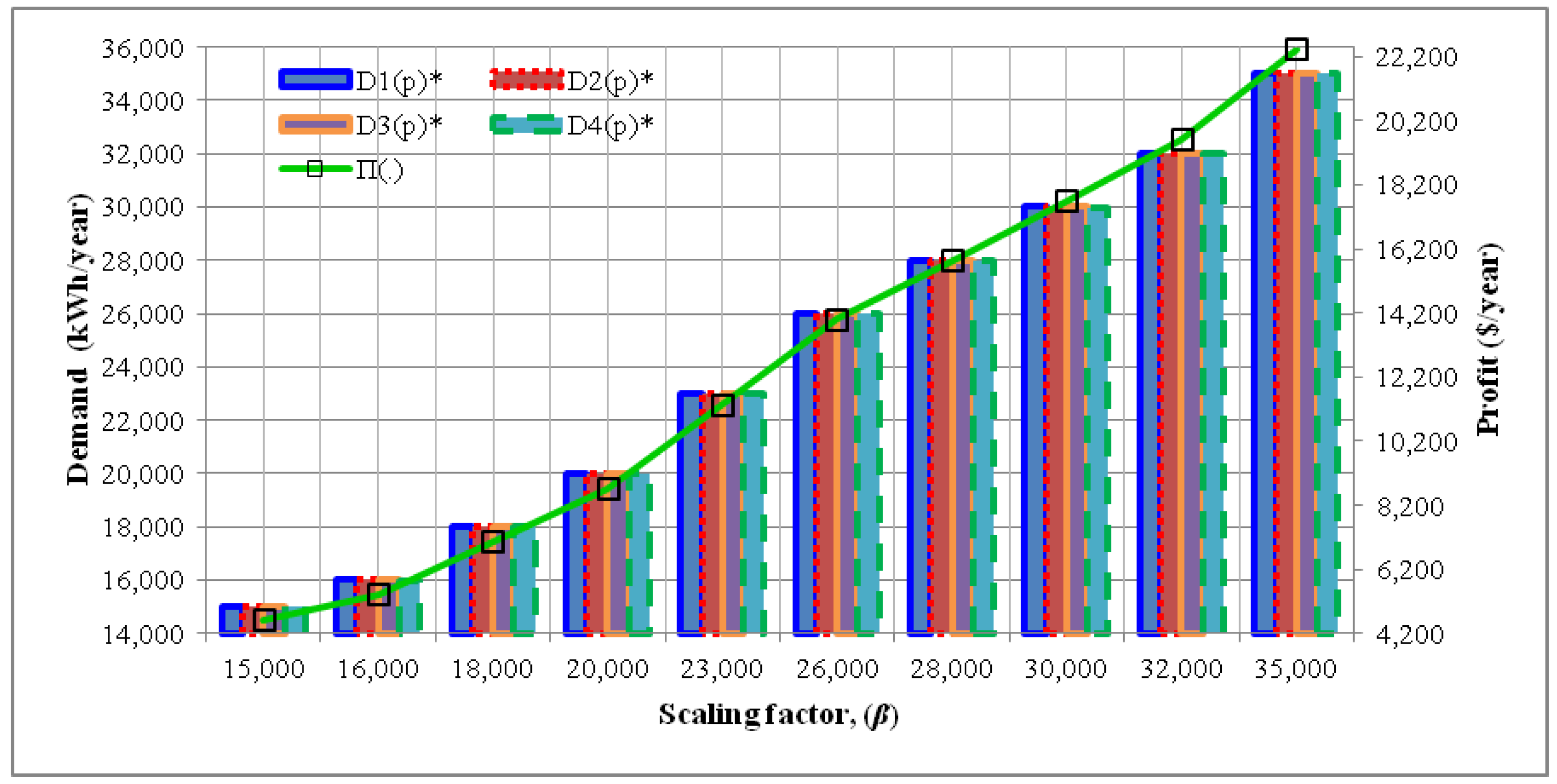
Table 7 and Figure 3 present the impact of the scaling factor of demand (β). The results are similar to the price elasticity coefficient on the optimal solutions. They show that when the scaling factor increases, consumer demand, power consumption, and total profit also increase. The parameters D1(p), D2(p), D3(p), D4(p), Q and Π increase (6.66% to 15%), (6.66% to 14.9%), (6.66% to 14.9%), (6.7% to 15%), (−8.2% to 8%), and (10.6% to 30%), respectively.
6.3. Price of Electricity (p)
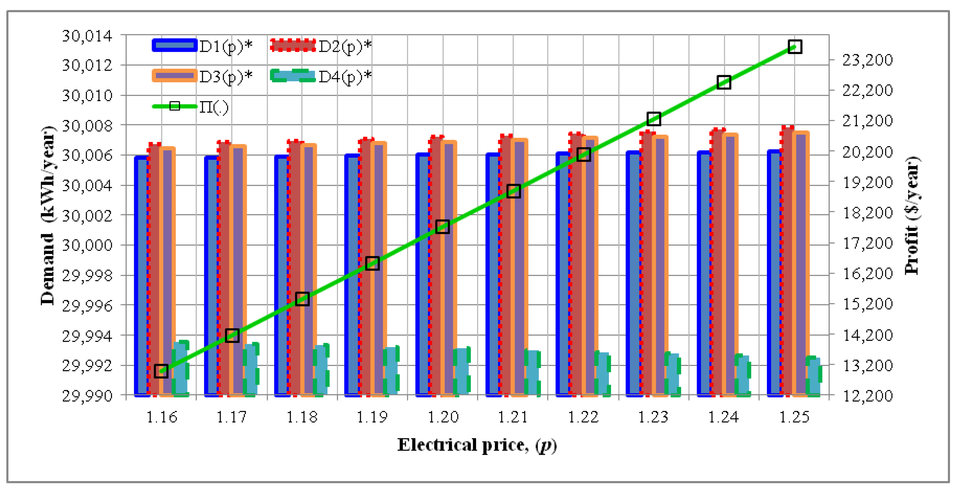
We examined the effects of changes in the price of electricity (p) starting from $1.16/kWh to $1.25/kWh. It must be noted that we kept the production cost at (v = $0.85/kWh). Table 8 and Figure 4 show that the results were not affected by changes in the customer demand function. The results show that the price of electricity is also not affected by optimal power consumption. If the price of electricity was to increase and the production cost was to remain unchanged, then the total profit would increase from 5.27% to 9.12%.
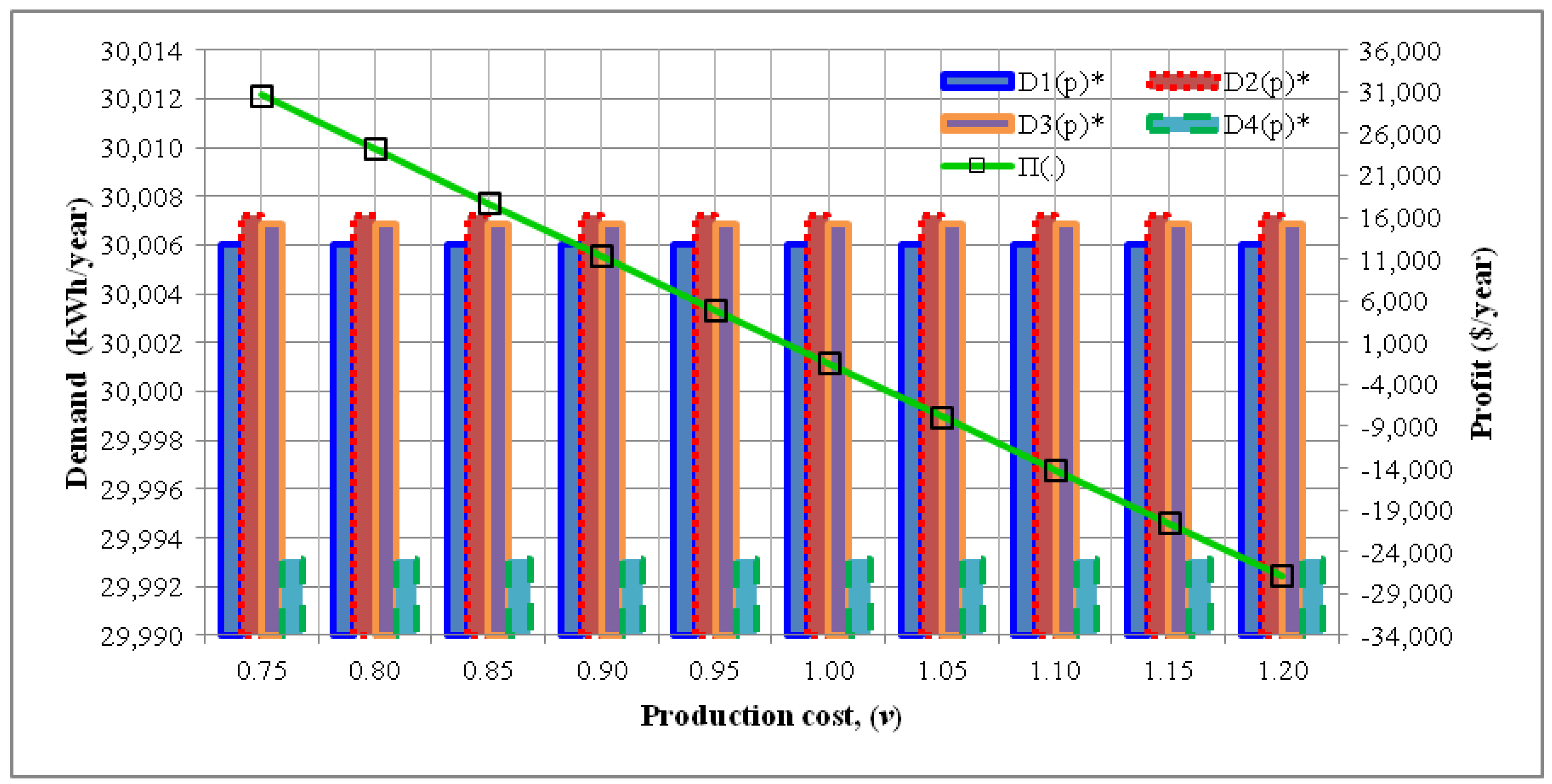
6.4. Production Cost (v)
Next, we examined the effects of changes in the production cost (v). In this case, we set the price of electricity to $1.20/kWh and production costs from $0.75/kWh to $1.10/kWh. We assumed that the production cost would not be more than the price of electricity (v < p). Table 9 and Figure 5 show that the customer demand function is similar to the price of electricity in that it is not affected by changes in production cost. In contrast, the results showed that the production cost is affected by the optimal power consumption, which decreases at an average of −0.36%. If the production cost increases and the price of electricity remains unchanged, then the total profit will decrease by −21.03% to −423.85%. Therefore, the profit resulting from the production cost is different from the profit resulting from the price of electricity.
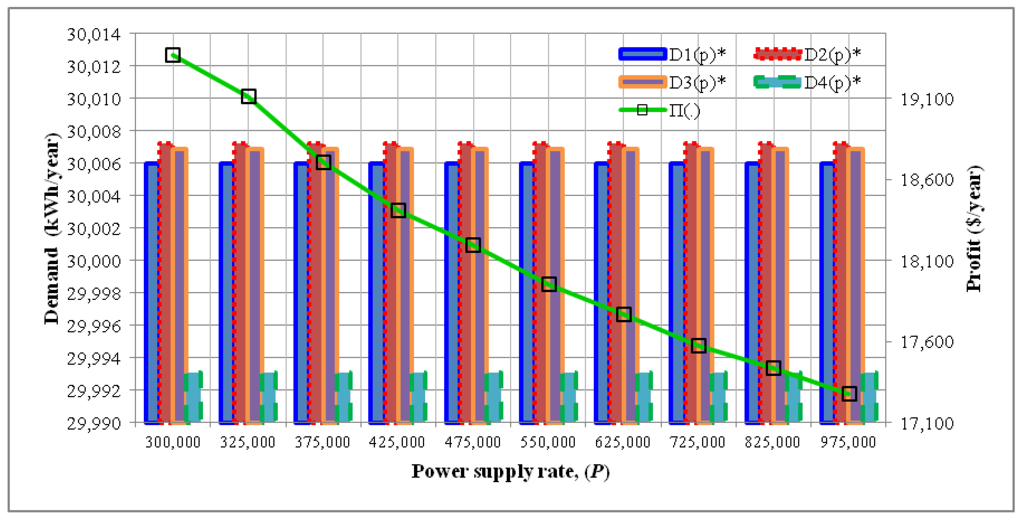
6.5. Power Supply Rate (P)
In addition, we examined the effects of changes in the power supply rate (P), assuming that it is higher than customer demand (P > D(p)). For example, we investigated changes in the power supply rate starting from 300,000 kWh/year, 325,000 kWh/year to 975,000 kWh/year. We found that if the power’s supply rate rises (the demand of the customers will be unchanged) the impact on total profit will decrease (average −0.41%), which is caused by the fact that if the holding cost of electricity increases, the power supply rate will also increase. However, if the power supply rate and customer demand of customer increase simultaneously, profitability increases. Further, we also analyze with some combination of parameters. The results are shown in Table 10 and Figure 6.
6.6. Effect of Changes on Combination of Parameters
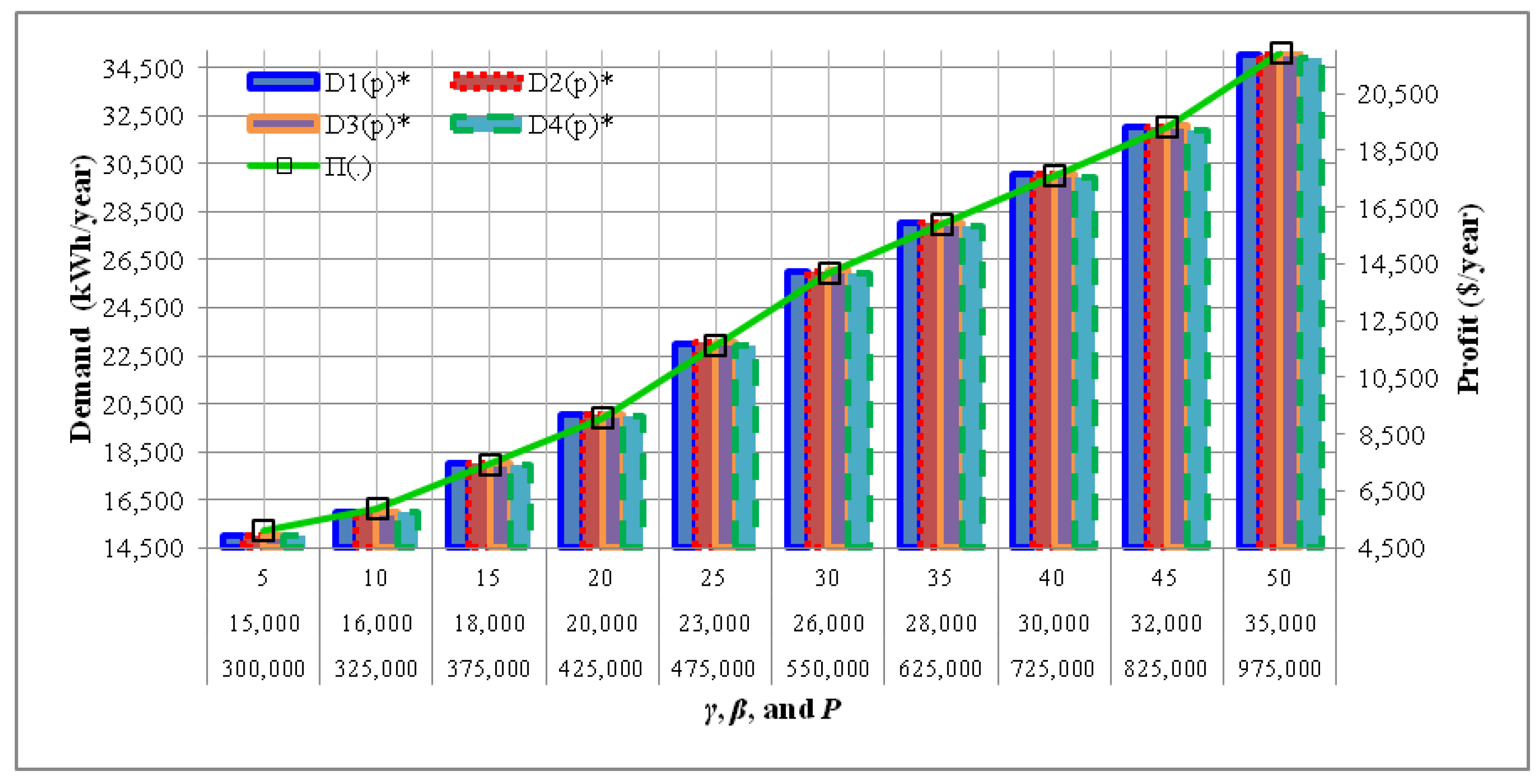
6.6.1. Price Elasticity Coefficient (γ), Scaling Factor (β), and Power Supply Rate (P)
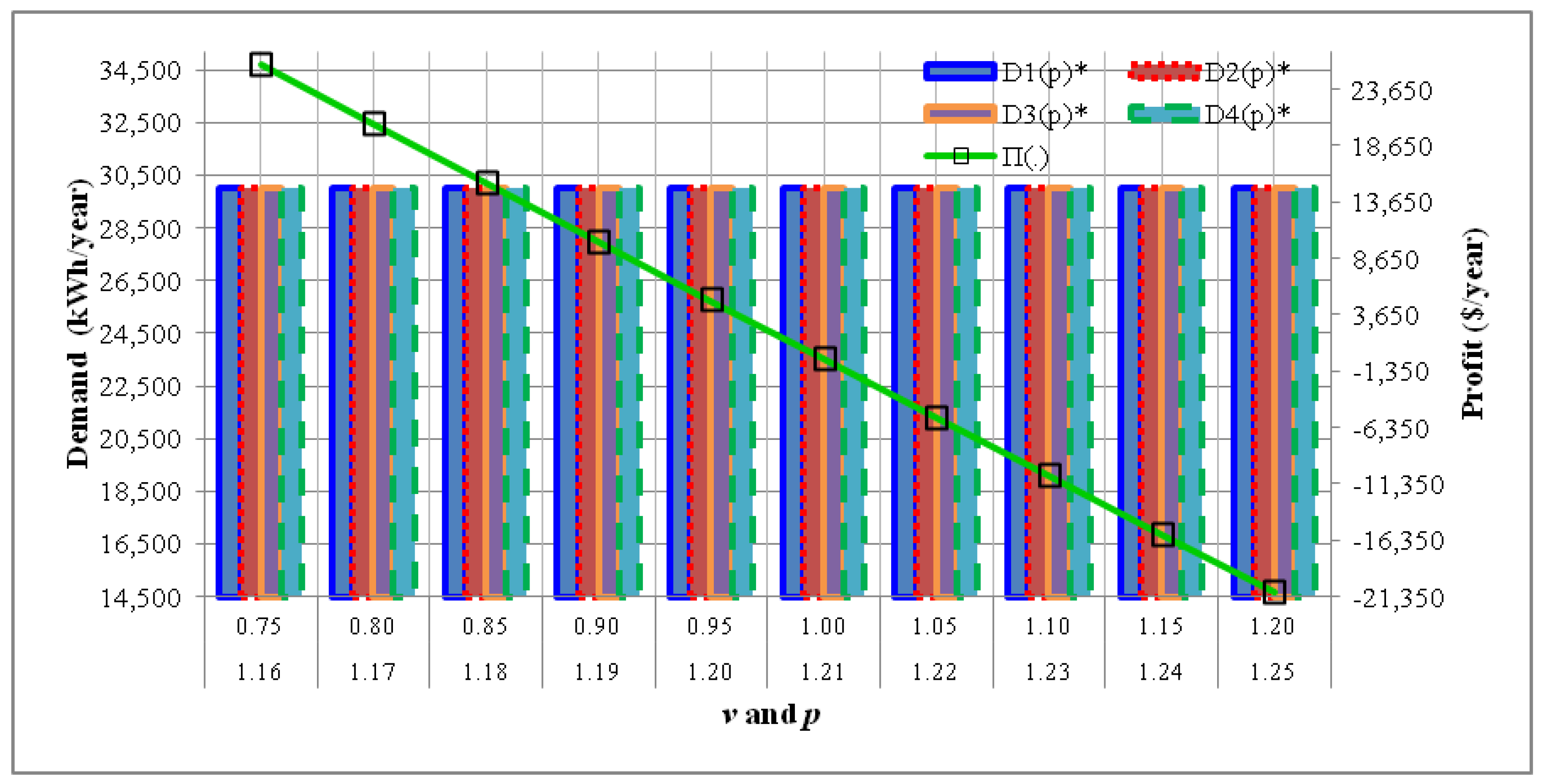
6.6.2. Price of Electricity (p) and Production Cost (v)
Last, we examined the effects of changes in the price of electricity (p) and production cost (v). Table 12 and Figure 8 show that if these variables increase simultaneously, this will cause a significant decrease (−20.30% to −1,633.38%) in total profits. The decrease of total profit is dependent on a stepwise decline in the price of electricity and production costs.
7. Conclusions, Managerial Implications and Directions for Future Research
In this paper, we propose a mathematical model thatassumes price-dependent customer demands. We define and examine four types of customer demands: namely demand may increase linearly, quadratically, multiplicatively or decreasing multiplicatively. The model developedis based on the inventory theory where we examine how the optimal decision variables and the total profits are affected by the price elasticity coefficient (γ), scaling factor (β), price of electricity (p), production cost (v) and the power supply rate (P) parameters.
The sensitivity analysis illustrates that the price elasticity coefficient (γ), scaling factor (β) and price of electricity (p) are significant in maximizing the profit. When the forementioned parametersincrease, the consumer demandsalso increase. When other parameters remain the same, it is obvious that the profit will decrease when the production cost (v) and power supply rate (P) increase. Based on our results, we provide insights to the production and marketing managers in designing a profitable and sustainable electrical energy supply chain.
For future study, researchers may wish to extend the proposed model to include mark-up pricing or subsidized electricity pricing. Scholars may also consider incorporating discount pricing strategies as well as the effect of carbon emissions. Moreover, researchers may wish to look into a more complex type of electrical supply chain, such as a multi-transmission and distribution substation.
Author Contributions
Conceptualization, H.-M.W.; Methodology, I.D.W. and T.-M.Y.; Software, n/a; Validation, I.D.W., T.-M.Y. and H.-M.W.; Formal Analysis, I.D.W.; Investigation, n/a; Resources, H.-M.W.; Data Curation, I.D.W. and T.-M.Y.; Writing-Original Draft Preparation, I.D.W.; Writing-Review & Editing, H.-M.W.; Visualization, n/a; Supervision, H.-M.W.; Project Administration, H.-M.W.; Funding Acquisition, n/a.
Funding
This research received no external funding.
Acknowledgments
The authors express their gratitude to the editor and the two anonymous reviewers for their comments and valuable suggestions to improve this paper.
Conflicts of Interest
The authors declare no conflict of interest.
Abbreviations
| Index | |
| i | the ith customer, i = 1, 2, …, N |
| Decision Variables | |
| Q | The customer’s power consumption, in kW. |
| g | The electrical power distribution factor’s effect on the distribution substation (integer). |
| n | The electrical power transmission factor’s impact on the transmission substation (integer). |
| m | The electrical power generation’s factor (integer). |
| Parameters | |
| D(p) | Customers’ average electrical demand rate, in kWh per year. |
| P | The power supply rate, in kWh per year. |
| t | Customer’s average electricity consumption in hour(s). |
| E | Customers’ average energy consumption, in kWh. |
| A | Cost per order in dollars. |
| S | Cost per setup of power generation in dollars. |
| p | Price of electricity in dollars per kWh. |
| v | Production cost, in dollars per kWh. |
| rt | Annual percent of holding cost rate per unit time of the transmission substation. |
| rp | Annual percent of holding cost rate per unit time of power generation. |
| Δ | Power factor correction in kVA per kWh. |
| Ct | The per mile transmission and distribution rates in dollars per kVA. |
| dd | The per mile transportation network from the distribution substation to the customers in miles. |
| dt | The per mile transportation network from the transmission substation to the distribution substation in miles. |
| dp | The per mile transportation network from power generation to the transmission substation in miles. |
| Wdx | Maximum capacity of the distribution substation in KVA. |
| Wtx | Maximum capacity of the transmission substation in KVA. |
| Wpx | Maximum capacity of power generation in KVA. |
| Wdy | Actual capacity of the distribution substation in KVA. |
| Wty | Actual capacity of the transmission substation in KVA. |
| Wpy | Actual capacity of the power generation capacity in KVA. |
| α | The power supply loss factor, 0 ≤ α ≤ 1. |
| β | The scaling factor, β > 0. |
| γ | The price elasticity coefficient, γ > 1. |
References
- U.S. Energy Information Administration. Today in Energy. Government Report. 2017. Available online: https://www.eia.gov/todayinenergy/detail.php?id=12251 (accessed on 1 April 2017).
- Banbury, J.G. Distribution-the final link in the electricity-supply chain. Electron. Power 1975, 21, 773–775. [Google Scholar] [CrossRef]
- Ventosa, M.; Baıllo, A.; Ramos, A.; Rivier, M. Electricity market modeling trends. Energy Policy 2005, 33, 897–913. [Google Scholar] [CrossRef]
- Paatero, J.V.; Lund, P.D. A model for generating household electricity load profiles. Int. J. Energy Res. 2006, 30, 273–290. [Google Scholar] [CrossRef] [Green Version]
- Tolis, A.I.; Rentizelas, A.A. An impact assessment of electricity and emission allowances pricing in optimized expansion planning of power sector portfolios. Appl. Energy 2011, 88, 3791–3806. [Google Scholar] [CrossRef] [Green Version]
- Genoese, F.; Genoese, M. Assessing the value of storage in a future energy system with a high share of renewable electricity generation. Energy Syst. 2014, 5, 19–44. [Google Scholar] [CrossRef]
- Pavković, D.; Hoić, M.; Deur, J.; Petrić, J. Energy storage systems sizing study for a high-altitude wind energy application. Energy 2014, 76, 91–103. [Google Scholar] [CrossRef]
- Schröder, A. An electricity market model with generation capacity expansion under uncertainty. Energy Syst. 2014, 5, 253–267. [Google Scholar] [CrossRef]
- Fossati, J.P.; Galarza, A.; Martín-Villate, A.; Fontán, L. A method for optimal sizing energy storage systems for microgrids. Renew. Energy 2015, 77, 539–549. [Google Scholar] [CrossRef]
- Luo, X.; Wang, J.; Dooner, M.; Clarke, J. Overview of current development in electrical energy storage technologies and the application potential in power system operation. Appl. Energy 2015, 137, 511–536. [Google Scholar] [CrossRef]
- Schneider, M.; Biel, K.; Pfaller, S.; Schaede, H.; Rinderknecht, S.; Glock, C.H. Optimal sizing of electrical energy storage systems using inventory models. Energy Procedia. 2015, 73, 48–58. [Google Scholar] [CrossRef]
- Schneider, M.; Biel, K.; Pfaller, S.; Schaede, H.; Rinderknecht, S.; Glock, C.H. Using inventory models for sizing energy storage systems: An interdisciplinary approach. J. Energy Storage 2016, 8, 339–348. [Google Scholar] [CrossRef]
- Taylor, J.A.; Mathieu, J.L.; Callaway, D.S.; Poolla, K. Price and capacity competition in balancing markets with energy storage. Energy Syst. 2017, 8, 169–197. [Google Scholar] [CrossRef]
- Wu, A.; Philpott, A.; Zakeri, G. Investment and generation optimization in electricity systems with intermittent supply. Energy Syst. 2017, 8, 127–147. [Google Scholar] [CrossRef]
- Ouedraogo, N.S. Modeling sustainable long-term electricity supply-demand in Africa. Appl. Energy 2017, 190, 1047–1067. [Google Scholar] [CrossRef]
- Wangsa, I.D.; Wee, H.M. The economical modelling of a distribution systemfor electricity supply chain. Energy Syst. 2018, 1–22. [Google Scholar] [CrossRef]
- Goyal, S.K. An integrated inventory model for a single supplier-single customer problem. Int. J. Prod. Res. 1977, 15, 107–111. [Google Scholar] [CrossRef]
- Banerjee, A. A joint economic-lot-size model for purchaser and vendor. Decis. Sci. 1986, 17, 292–311. [Google Scholar] [CrossRef]
- Goyal, S.K. A joint economic-lot-size model for purchaser and vendor: A comment. Decis. Sci. 1988, 19, 236–241. [Google Scholar] [CrossRef]
- Goyal, S.K. A one-vendor multi-buyer integrated inventory model: A comment. Eur. J. Oper. Res. 1995, 82, 209–210. [Google Scholar] [CrossRef]
- Lu, L. A one-vendor multi-buyer integrated inventory model. Eur. J. Oper. Res. 1995, 81, 312–323. [Google Scholar] [CrossRef]
- Hill, R.M. The single-vendor single-buyer integrated production-inventory model with a generalized policy. Eur. J. Oper. Res. 1997, 97, 493–499. [Google Scholar] [CrossRef]
- Hill, R.M. The optimal production and shipment policy for the single-vendor single-buyer integrated production-inventory problem. Int. J. Prod. Res. 1999, 37, 2463–2475. [Google Scholar] [CrossRef]
- Hariga, M.; Ben-Daya, M. Some stochastic inventory models with deterministic variable lead time. Eur. J. Oper. Res. 1999, 113, 42–51. [Google Scholar] [CrossRef]
- Pan, J.C.H.; Yang, J.S. A study of an integrated inventory with controllable lead time. Int. J. Prod. Res. 2002, 40, 1263–1273. [Google Scholar] [CrossRef]
- Jauhari, W.A.; Pujawan, I.N.; Wiratno, S.E.; Priyandari, Y. Integrated inventory model for single vendor–single buyer with probabilistic demand. Int. J. Oper. Res. 2011, 11, 160–178. [Google Scholar] [CrossRef]
- Wangsa, I.D.; Wee, H.M. An integrated vendor-buyer inventory model with transportation cost and stochastic demand. Int. J. Syst. Sci. Oper. Logist. 2017. [Google Scholar] [CrossRef]
- Swenseth, S.R.; Buffa, F.P. Just-in-time: Some effects on the logistics function. Int. J. Logist. Manag. 1990, 1, 25–34. [Google Scholar] [CrossRef]
- Swenseth, S.R.; Godfrey, M.R. Incorporating transportation costs into inventory replenishment decisions. Int. J. Prod. Econ. 2002, 77, 113–130. [Google Scholar] [CrossRef]
Figure 1.
The analogies between Sustainable Electrical Supply Chain System (SESCS) and Supply Chain Inventory System (SCIS).
Figure 1.
The analogies between Sustainable Electrical Supply Chain System (SESCS) and Supply Chain Inventory System (SCIS).

Figure 2.
The Effect of Changes in the Price Elasticity Coefficient on Profitand Demand.

Figure 3.
The Effect of Changes in the Scaling Factor on Profitand Demand.

Figure 4.
The Effect of Changes in the Price of Electricity on Profitand Demand.

Figure 5.
The Effect of Changes in the Production Cost on Profitand Demand.

Figure 6.
The Effect of Changes in the Power Supply Rate on Profitand Demand.

Figure 7.
The Effect of Simultaneous Changes in the Power Supply Rate, Scaling Factor and Price Elasticity Coefficient on Profitand Demand.
Figure 7.
The Effect of Simultaneous Changes in the Power Supply Rate, Scaling Factor and Price Elasticity Coefficient on Profitand Demand.

Figure 8.
The Effect of Simultaneous Changes in the Price of Electricity and Production Cost on Profitand Demand.
Figure 8.
The Effect of Simultaneous Changes in the Price of Electricity and Production Cost on Profitand Demand.


Table 1.
Customer Data.
| Parameter | Customer | |||
|---|---|---|---|---|
| 1 | 2 | 3 | 4 | |
| Types of Demand Function | Increasing | Increasing | Increasing | Decreasing |
| Linear | Quadratic | Multiplicative | Multiplicative | |
| Demand Function | ||||
| Scaling Factor | 30,000 | 30,000 | 30,000 | 30,000 |
| Price Elasticity Coefficient | 5 | 5 | 5 | 5 |
| Avg. Time of Electrical Consumption (hours) | 24 | 24 | 24 | 24 |
| Ordering Cost ($) | 20 | 20 | 20 | 20 |
| Price of Electricity($/kWh) | 1.20 | 1.20 | 1.20 | 1.20 |
| Holding Cost Rate (%/year) | 0.20 | 0.20 | 0.20 | 0.20 |
| Power Supply Loss Factor | 0.1125 | 0.1125 | 0.1125 | 0.1125 |
| Power Factor Correction (kVA/kWh) | 1.25 | 1.25 | 1.25 | 1.25 |
Table 2.
Power Generation, Transmission Substation and Distribution Substation Data.
| Parameters | Power Generation | Transmission Substation | Distribution Substation |
|---|---|---|---|
| Power Supply Rate (kWh/year) | 650,000 | - | - |
| Production Cost ($/kWh) | 0.85 | - | - |
| Setup Cost ($) | 5600 | - | - |
| Holding Cost Rate of the Power Generation (%/year) | 0.20 | - | - |
| Transmission and Distribution Rates ($/kVA/mile) | 0.000455 | - | - |
| Maximum Capacity of Power Generation (kVA) | 500,000 | - | - |
| Maximum Capacity of Transmission Substation (kVA) | - | 350,000 | - |
| Maximum Capacity of Distribution Substation (kVA) | - | - | 10,500 |
Table 3.
The Network Data for Power Generation, and Transmission and Distribution Substations.
| From—To | Transmission Substation | Distribution Substation | Customers |
|---|---|---|---|
| Power Generation (miles) | 80 | - | - |
| Transmission Substation (miles) | - | 10 | - |
| Distribution Substation (miles) | - | - | 3 |
Table 4.
Details of the Procedures for this Example.
| m | n* | g* | D1(p)* | D2(p)* | D3(p)* | D4(p)* | Q* | * | Q* Revisited | * | * | Π(.) |
|---|---|---|---|---|---|---|---|---|---|---|---|---|
| 1 | 10 | 1 | 30,006.0 | 30,007.2 | 30,006.9 | 29,993.1 | 351.42 | 10,542.59 | 350.00 | 105,000.00 | 105,000.00 | 13,481.57 |
| 2 | 6 | 1 | 30,006.0 | 30,007.2 | 30,006.9 | 29,993.1 | 341.57 | 10,247.24 | 341.57 | 61,483.45 | 122,966.91 | 16,204.24 |
| 3 | 4 | 1 | 30,006.0 | 30,007.2 | 30,006.9 | 29,993.1 | 365.55 | 10,966.51 | 350.00 | 42,000.00 | 126,000.00 | 17,100.27 |
| 4 | 3 | 1 | 30,006.0 | 30,007.2 | 30,006.9 | 29,993.1 | 381.12 | 11,433.53 | 350.00 | 31,500.00 | 126,000.00 | 17,444.63 |
| 5 | 3 | 1 | 30,006.0 | 30,007.2 | 30,006.9 | 29,993.1 | 315.33 | 9459.89 | 315.33 | 28,379.68 | 141,898.39 | 17,621.25 |
| 6 | 3 | 1 | 30,006.0 | 30,007.2 | 30,006.9 | 29,993.1 | 270.01 | 8100.23 | 270.01 | 24,300.69 | 145,804.12 | 17,621.42 |
| 7 | 2 | 1 | 30,006.0 | 30,007.2 | 30,006.9 | 29,993.1 | 352.40 | 10,571.91 | 350.00 | 21,000.00 | 147,000.00 | 17,712.07 ← |
| 8 | 2 | 1 | 30,006.0 | 30,007.2 | 30,006.9 | 29,993.1 | 314.42 | 9432.73 | 314.42 | 18,865.46 | 150,923.72 | 17,631.05 |
* the local solution; ←the optimal solution.
Table 5.
The Results.
| Decision Variables | Values |
|---|---|
| Demand of Customer 1 | 30,006.00 kWh/year |
| Demand of Customer 2 | 30,007.20 kWh/year |
| Demand of Customer 3 | 30,006.90 kWh/year |
| Demand of Customer 4 | 29,993.10 kWh/year |
| Electrical power consumption of Customer 1 | 87.51 kW |
| Electrical power consumption of Customer 2 | 87.51 kW |
| Electrical power consumption of Customer 3 | 87.51 kW |
| Electrical power consumption of Customer 4 | 87.47 kW |
| Electrical power Generation | 7 times |
| Electrical power transmission factor | 2 times |
| Electrical power distribution factor | 1 times |
| Energy transmitted by Power Generation | 117,600.00 kWh |
| Energy transmitted by Transmission Substation | 16,800.00 kWh |
| Energy transmitted by Distribution Substation | 8400.00 kWh |
| Energy consumed by Customer 1 | 2100.19 kWh |
| Energy consumed by Customer 2 | 2100.27 kWh |
| Energy consumed by Customer 3 | 2100.25 kWh |
| Energy consumed by Customer 4 | 2099.29 kWh |
| Actual capacity of Power Generation | 147,000.00 kVA |
| Actual capacity of Transmission Substation | 21,000.00 kVA |
| Actual capacity of Distribution Substation | 10,571.91 kVA |
Table 6.
Effect of Changes in the Price Elasticity Coefficient Parameter.
| Price ElasticityCoefficient, (γ) | m * | n * | g * | D1(p) * | D2(p) * | D3(p) * | D4(p) * | Q * | Π(.) |
|---|---|---|---|---|---|---|---|---|---|
| 5 | 7 | 2 | 1 | 30,006.00 | 30,007.20 | 30,006.90 | 29,993.10 | 350.00 | 17,712.07 |
| 10 | 7 | 2 | 1 | 30,012.00 | 30,014.40 | 30,015.85 | 29,984.15 | 350.00 | 17,715.19 |
| 15 | 7 | 2 | 1 | 30,018.00 | 30,021.60 | 30,025.78 | 29,974.22 | 350.00 | 17,718.30 |
| 20 | 7 | 2 | 1 | 30,024.00 | 30,028.80 | 30,036.41 | 29,963.59 | 350.00 | 17,721.41 |
| 25 | 7 | 2 | 1 | 30,030.00 | 30,036.00 | 30,047.59 | 29,952.41 | 350.00 | 17,724.52 |
| 30 | 7 | 2 | 1 | 30,036.00 | 30,043.20 | 30,059.23 | 29,940.77 | 350.00 | 17,727.64 |
| 35 | 7 | 2 | 1 | 30,042.00 | 30,050.40 | 30,071.27 | 29,928.73 | 350.00 | 17,730.75 |
| 40 | 7 | 2 | 1 | 30,048.00 | 30,057.60 | 30,083.65 | 29,916.35 | 350.00 | 17,733.86 |
| 45 | 7 | 2 | 1 | 30,054.00 | 30,064.80 | 30,096.35 | 29,903.65 | 350.00 | 17,736.97 |
| 50 | 7 | 2 | 1 | 30,060.00 | 30,072.00 | 30,109.34 | 29,890.66 | 350.00 | 17,740.08 |
* the local solution.
Table 7.
Effect of Changes in the Scaling Factor Parameter.
| Scaling Factor, (β) | m * | n * | g * | D1(p) * | D2(p) * | D3(p) * | D4(p) * | Q * | Π(.) |
|---|---|---|---|---|---|---|---|---|---|
| 15,000 | 5 | 2 | 1 | 15,006.00 | 15,007.20 | 15,006.90 | 14,993.10 | 323.34 | 4639.38 |
| 16,000 | 5 | 2 | 1 | 16,006.00 | 16,007.20 | 16,006.90 | 15,993.10 | 334.55 | 5432.56 |
| 18,000 | 5 | 2 | 1 | 18,006.00 | 18,007.20 | 18,006.90 | 17,993.10 | 350.00 | 7061.27 |
| 20,000 | 6 | 2 | 1 | 20,006.00 | 20,007.20 | 20,006.90 | 19,993.10 | 321.44 | 8722.39 |
| 23,000 | 6 | 2 | 1 | 23,006.00 | 23,007.20 | 23,006.90 | 22,993.10 | 346.87 | 11,339.64 |
| 26,000 | 6 | 2 | 1 | 26,006.00 | 26,007.20 | 26,006.90 | 25,993.10 | 350.00 | 14,011.84 |
| 28,000 | 7 | 2 | 1 | 28,006.00 | 28,007.20 | 28,006.90 | 27,993.10 | 338.85 | 15,835.38 |
| 30,000 | 7 | 2 | 1 | 30,006.00 | 30,007.20 | 30,006.90 | 29,993.10 | 350.00 | 17,712.07 |
| 32,000 | 7 | 2 | 1 | 32,006.00 | 32,007.20 | 32,006.90 | 31,993.10 | 350.00 | 19,598.27 |
| 35,000 | 8 | 2 | 1 | 35,006.00 | 35,007.20 | 35,006.90 | 34,993.10 | 343.99 | 22,448.29 |
* the local solution.
Table 8.
Effect of Changes in the Price of Electricity Parameter.
| Price of Electricity, (p) | m * | n * | g * | D1(p) * | D2(p) * | D3(p) * | D4(p) * | Q * | Π(.) |
|---|---|---|---|---|---|---|---|---|---|
| 1.16 | 7 | 2 | 1 | 30,005.80 | 30,006.73 | 30,006.47 | 29,993.53 | 350.00 | 12,978.61 |
| 1.17 | 7 | 2 | 1 | 30,005.85 | 30,006.84 | 30,006.57 | 29,993.43 | 350.00 | 14,161.97 |
| 1.18 | 7 | 2 | 1 | 30,005.90 | 30,006.96 | 30,006.68 | 29,993.32 | 350.00 | 15,345.34 |
| 1.19 | 7 | 2 | 1 | 30,005.95 | 30,007.08 | 30,006.79 | 29,993.21 | 350.00 | 16,528.70 |
| 1.20 | 7 | 2 | 1 | 30,006.00 | 30,007.20 | 30,006.90 | 29,993.10 | 350.00 | 17,712.07 |
| 1.21 | 7 | 2 | 1 | 30,006.05 | 30,007.32 | 30,007.01 | 29,992.99 | 350.00 | 18,895.45 |
| 1.22 | 7 | 2 | 1 | 30,006.10 | 30,007.44 | 30,007.12 | 29,992.88 | 350.00 | 20,078.83 |
| 1.23 | 7 | 2 | 1 | 30,006.15 | 30,007.56 | 30,007.24 | 29,992.76 | 350.00 | 21,262.21 |
| 1.24 | 7 | 2 | 1 | 30,006.20 | 30,007.69 | 30,007.36 | 29,992.64 | 350.00 | 22,445.59 |
| 1.25 | 7 | 2 | 1 | 30,006.25 | 30,007.81 | 30,007.48 | 29,992.52 | 350.00 | 23,628.98 |
* the local solution.
Table 9.
Effect of Changes in the Production Cost Parameter.
| Production Cost, (v) | m * | n * | g * | D1(p) * | D2(p) * | D3(p) * | D4(p) * | Q * | Π(.) |
|---|---|---|---|---|---|---|---|---|---|
| 0.75 | 7 | 2 | 1 | 30,006.00 | 30,007.20 | 30,006.90 | 29,993.10 | 350.00 | 30,566.30 |
| 0.80 | 7 | 2 | 1 | 30,006.00 | 30,007.20 | 30,006.90 | 29,993.10 | 350.00 | 24,139.19 |
| 0.85 | 7 | 2 | 1 | 30,006.00 | 30,007.20 | 30,006.90 | 29,993.10 | 350.00 | 17,712.07 |
| 0.90 | 7 | 2 | 1 | 30,006.00 | 30,007.20 | 30,006.90 | 29,993.10 | 344.56 | 11,287.31 |
| 0.95 | 7 | 2 | 1 | 30,006.00 | 30,007.20 | 30,006.90 | 29,993.10 | 337.22 | 4871.34 |
| 1.00 | 6 | 2 | 1 | 30,006.00 | 30,007.20 | 30,006.90 | 29,993.10 | 350.00 | −1500.19 |
| 1.05 | 6 | 2 | 1 | 30,006.00 | 30,007.20 | 30,006.90 | 29,993.10 | 350.00 | −7858.81 |
| 1.10 | 4 | 3 | 1 | 30,006.00 | 30,007.20 | 30,006.90 | 29,993.10 | 349.16 | −14,215.97 |
| 1.15 | 4 | 3 | 1 | 30,006.00 | 30,007.20 | 30,006.90 | 29,993.10 | 343.69 | −20,544.70 |
| 1.20 | 4 | 3 | 1 | 30,006.00 | 30,007.20 | 30,006.90 | 29,993.10 | 338.46 | −26,868.36 |
* the local solution.
Table 10.
Effect of Changes in the Power Supply Rate Parameter.
| Power Supply Rate, (P) | m * | n * | g * | D1(p) * | D2(p) * | D3(p) * | D4(p) * | Q* | Π(.) |
|---|---|---|---|---|---|---|---|---|---|
| 300,000 | 8 | 2 | 1 | 30,006.00 | 30,007.20 | 30,006.90 | 29,993.10 | 346.58 | 19,369.73 |
| 325,000 | 8 | 2 | 1 | 30,006.00 | 30,007.20 | 30,006.90 | 29,993.10 | 341.38 | 19,110.62 |
| 375,000 | 8 | 2 | 1 | 30,006.00 | 30,007.20 | 30,006.90 | 29,993.10 | 333.52 | 18,703.94 |
| 425,000 | 7 | 2 | 1 | 30,006.00 | 30,007.20 | 30,006.90 | 29,993.10 | 350.00 | 18,410.00 |
| 475,000 | 7 | 2 | 1 | 30,006.00 | 30,007.20 | 30,006.90 | 29,993.10 | 350.00 | 18,197.76 |
| 550,000 | 7 | 2 | 1 | 30,006.00 | 30,007.20 | 30,006.90 | 29,993.10 | 350.00 | 17,951.76 |
| 625,000 | 7 | 2 | 1 | 30,006.00 | 30,007.20 | 30,006.90 | 29,993.10 | 350.00 | 17,764.81 |
| 725,000 | 7 | 2 | 1 | 30,006.00 | 30,007.20 | 30,006.90 | 29,993.10 | 349.83 | 17,575.70 |
| 825,000 | 7 | 2 | 1 | 30,006.00 | 30,007.20 | 30,006.90 | 29,993.10 | 347.20 | 17,433.05 |
| 975,000 | 7 | 2 | 1 | 30,006.00 | 30,007.20 | 30,006.90 | 29,993.10 | 344.33 | 17,275.19 |
* the local solution.
Table 11.
Effect of Changes on Power Supply Rate, Scaling Factor, and Price Elasticity Coefficient Parameters.
Table 11.
Effect of Changes on Power Supply Rate, Scaling Factor, and Price Elasticity Coefficient Parameters.
| Power Supply Rate, (P) | Scaling Factor, (β) | Price Elasticity Coefficient, (γ) | m * | n * | g * | D1(p) * | D2(p) * | D3(p) * | D4(p) * | Q* | Π(.) |
|---|---|---|---|---|---|---|---|---|---|---|---|
| 300,000 | 15,000 | 5 | 6 | 2 | 1 | 15,006.00 | 15,007.20 | 15,006.90 | 14,993.10 | 285.91 | 5095.24 |
| 325,000 | 16,000 | 10 | 6 | 2 | 1 | 16,012.00 | 16,014.40 | 16,015.85 | 15,984.15 | 295.00 | 5866.16 |
| 375,000 | 18,000 | 15 | 6 | 2 | 1 | 18,018.00 | 18,021.60 | 18,025.78 | 17,974.22 | 312.37 | 7447.45 |
| 425,000 | 20,000 | 20 | 6 | 2 | 1 | 20,024.00 | 20,028.80 | 20,036.41 | 19,963.59 | 328.85 | 9076.85 |
| 475,000 | 23,000 | 25 | 6 | 2 | 1 | 23,030.00 | 23,036.00 | 23,047.59 | 22,952.41 | 350.00 | 11,648.80 |
| 550,000 | 26,000 | 30 | 7 | 2 | 1 | 26,036.00 | 26,043.20 | 26,059.23 | 25,940.77 | 328.75 | 14,197.13 |
| 625,000 | 28,000 | 35 | 7 | 2 | 1 | 28,042.00 | 28,050.40 | 28,071.27 | 27,928.73 | 339.88 | 15,901.58 |
| 725,000 | 30,000 | 40 | 7 | 2 | 1 | 30,048.00 | 30,057.60 | 30,083.65 | 29,916.35 | 349.98 | 17,597.38 |
| 825,000 | 32,000 | 45 | 7 | 2 | 1 | 32,054.00 | 32,064.80 | 32,096.35 | 31,903.65 | 350.00 | 19,324.64 |
| 975,000 | 35,000 | 50 | 5 | 3 | 1 | 35,060.00 | 35,072.00 | 35,109.34 | 34,890.66 | 336.51 | 21,953.34 |
* the local solution.
Table 12.
Effect of Changes in the Price of Electricity and Production Cost Parameters.
| Electrical Price, (p) | Production Cost, (v) | m * | n * | g * | D1(p) * | D2(p) * | D3(p) * | D4(p) * | Q * | Π(.) |
|---|---|---|---|---|---|---|---|---|---|---|
| 1.16 | 0.75 | 7 | 2 | 1 | 30,005.80 | 30,006.73 | 30,006.47 | 29,993.53 | 350.00 | 25,832.77 |
| 1.17 | 0.80 | 7 | 2 | 1 | 30,005.85 | 30,006.84 | 30,006.57 | 29,993.43 | 350.00 | 20,589.06 |
| 1.18 | 0.85 | 7 | 2 | 1 | 30,005.90 | 30,006.96 | 30,006.68 | 29,993.32 | 350.00 | 15,345.34 |
| 1.19 | 0.90 | 7 | 2 | 1 | 30,005.95 | 30,007.08 | 30,006.79 | 29,993.21 | 344.86 | 10,103.69 |
| 1.20 | 0.95 | 7 | 2 | 1 | 30,006.00 | 30,007.20 | 30,006.90 | 29,993.10 | 337.22 | 4871.34 |
| 1.21 | 1.00 | 6 | 2 | 1 | 30,006.05 | 30,007.32 | 30,007.01 | 29,992.99 | 350.00 | −316.84 |
| 1.22 | 1.05 | 6 | 2 | 1 | 30,006.10 | 30,007.44 | 30,007.12 | 29,992.88 | 350.00 | −5492.13 |
| 1.23 | 1.10 | 6 | 2 | 1 | 30,006.15 | 30,007.56 | 30,007.24 | 29,992.76 | 350.00 | −10,667.44 |
| 1.24 | 1.15 | 6 | 2 | 1 | 30,006.20 | 30,007.69 | 30,007.36 | 29,992.64 | 350.00 | −15,842.75 |
| 1.25 | 1.20 | 4 | 3 | 1 | 30,006.25 | 30,007.81 | 30,007.48 | 29,992.52 | 336.53 | −20,989.26 |
* the local solution.
© 2018 by the authors. Licensee MDPI, Basel, Switzerland. This article is an open access article distributed under the terms and conditions of the Creative Commons Attribution (CC BY) license (http://creativecommons.org/licenses/by/4.0/).
Share and Cite
MDPI and ACS Style
Wangsa, I.D.; Yang, T.M.; Wee, H.M. The Effect of Price-Dependent Demand on the Sustainable Electrical Energy Supply Chain. Energies 2018, 11, 1645. https://doi.org/10.3390/en11071645
AMA Style
Wangsa ID, Yang TM, Wee HM. The Effect of Price-Dependent Demand on the Sustainable Electrical Energy Supply Chain. Energies. 2018; 11(7):1645. https://doi.org/10.3390/en11071645
Chicago/Turabian StyleWangsa, Ivan Darma, Tao Ming Yang, and Hui Ming Wee. 2018. "The Effect of Price-Dependent Demand on the Sustainable Electrical Energy Supply Chain" Energies 11, no. 7: 1645. https://doi.org/10.3390/en11071645
Note that from the first issue of 2016, this journal uses article numbers instead of page numbers. See further details here.