Lithium-Ion Battery Prognostics with Hybrid Gaussian Process Function Regression

Abstract

The accurate prognostics of lithium-ion battery state of health (SOH) and remaining useful life (RUL) have great significance for reducing the costs of maintenance. The methods based on the physical models cannot perform satisfactorily as the systems become more and more complex. With the development of digital acquisition and storage technology, the data of battery cells can be obtained. This makes the data-driven methods get more and more attention. In this paper, to overcome the problem that the trend fitting deteriorates rapidly when test data are far from the training data for multiple-step-ahead estimation, a prognostic method fusing the wavelet de-noising (WD) method and the hybrid Gaussian process function regression (HGPFR) model for predicting the RUL of the lithium-ion battery is proposed. Gaussian process regression (GPR) is a typical representative for the Bayesian structure with non-parameter expression and uncertainty presentation. In this case, the effects on predictive results are compared and analyzed using the proposed method and the HGPFR model with different lengths of training data. Besides, in consideration of the degradation characteristics for the lithium-ion battery data set, the selections of the wavelet de-noising method are performed with corresponding experimental analyses. Furthermore, we set the hype-parameter for the mean function and co-variance function, and then develop a method for parameter optimization to make the proposed model suitable for the data. Moreover, a numerical simulation based on the data repository of Department of Engineering Science (DES) university of Oxford and Center for Advanced Life Cycle Engineering (CALCE) of University of Maryland is carried out, and the results are analyzed. For the data repository, an accuracy of 2.2% is obtained compared with the same value of 6.7% for the HGPFR model. What is more, the applicability and stability are verified with the prognostic results by the proposed method.

1. Introduction

Lithium-ion batteries are used to enable main equipment to store electricity, with the advantages of high specific energy, long service life, high reliability, and safety [1]. These advantages promote the application of lithium-ion batteries in battery-powered systems [2], such as mobile phones, laptops, electric vehicles, etc. Moreover, applications have been extended to the fields of military communications and aerospace [3]. Lithium-ion batteries have gradually become the key technology in many crucial fields [4,5].

However, as a lithium-ion battery cell ages, the power fades, the capacity fades, and other performance degradation occurs [6]. To specify the performance of the lithium-ion battery under uncertain situations, lithium-ion batteries are usually chosen with over-capacity [7,8]. On the one hand, this costs more. On the other hand, it is a pivotal part of the battery management system (BMS) with high prediction accuracy. At present, many studies are concentrated on the estimation of the state of charge (SOC) [8,9,10], the state of health (SOH) [4,11] and remaining useful life (RUL) [1,2,3] for lithium-ion batteries.

For the conventional methods, the prognostic models are constructed based on the equivalent circuit models, such as the battery internal resistance equivalent (Rint) model, the Thevenin model, the partnership for a new generation of vehicles (PNGV) model, the General-nonlinear (GNL) model, etc. [12,13]. These methods can describe the working principle and physical interpretation of the lithium-ion battery. There are many studies about prognostic models based on the equivalent circuit models. For instance, Ref. [13] propose an approach based on the RC equivalent circuit model for the SOC prediction. This paper has got some satisfied results that are based on the specified working conditions. However, the relationship between the number of RC networks and model accuracy remains unresolved. In fact, with the increment of RC networks, the accuracy of model may not be better [14]. Worse more, excessive RC networks increase the complexity of the model. On the one hand, the performance of lithium-ion battery is directly related to its aging state and operating temperature. On the other hand, the practical working condition is so complex that the equivalent circuit models cannot represent the degradation behavior accurately.

To overcome the problem with equivalent circuit model, the prognostic model based on the data-driven method is getting more and more attention. It is a vital characteristic that the data-driven methods are non-parametric. Hence, these approaches can be used for predicting the state of complex battery system, if there are sufficient data and the accuracy of the data-driven method depends on the size of data. There are many studies for battery prediction based on data-driven methods, such as the particle filter (PF), the relevance vector machine (RVM), the support vector machine (SVM), the Kalman filter (KF), etc. Ref. [15] propose a method depending on the unscented particle filter (UPF) for the prognostics of RUL. In this paper, the proposed method is modeled by understanding the degradation of the battery, and the results are obtained with 5% maximum error. Hu Chao et al. [16] applied the RVM and a specified model for the battery aging for the prediction of lithium-ion battery capacity. Zou et al. [17] propose a multi-time-scale method based on extended Kalman filter (EKF) and unscented Kalman filter (UKF) for estimating the SOC and SOH of lithium-ion battery. Besides, the authors of Ref. [17] obtain higher robustness and accuracy. Wei et al. [18] apply an online prediction model for improving the performance of vanadium redox battery (VRB), and the parameters are optimized with recursive least squares (RLS) and EKF. Furthermore, for the certain prediction time horizon, the constraints containing current, SOC, and voltage are incorporated with the estimation of the peak power in real time.

However, there is still a problem of weak prediction ability for the data-driven method supporting uncertainty presentation [19]. In addition, the battery resistance is used for the health index (HI) for the research of the lithium-ion battery RUL estimation [20]. Besides, it is very difficult to monitor and measure the battery resistance. Worse more, the rated capacity is also difficult to measure and estimate under fully charged or discharged conditions [21]. The Bayesian models have a pivotal characteristic with uncertainty presentation. The results of Bayesian models provide the confidence bounds that help make better decisions [22,23]. Compared with other data-driven methods, the GPR method is a type of Bayesian model that has exclusive strength. At the same time, the GPR method can also improve the accuracy of estimation without the physical model.

In recent years, the models based on GPR have been used for the battery estimation. Ref. [24] propose a method based on the GPR model for predicting the battery capacity through calculating the value of internal resistance. However, the method proposed by Ref. [24] is modeled on the condition that the relationship of mapping internal resistance to capacity is linear. When applied practically, this cannot guarantee that the relationship between internal resistance and capacity is linear. Moreover, the short-term prognostics have been shown only, and they are lacking in terms of long-term prediction. Ref. [25] propose a method for SOH prediction with combination of Gaussian process and PF. For that paper, the data on different working conditions are used for training data to fit the battery degradation, and the parameters are optimized by the maximization of the log-likelihood, and high accuracy is obtained. Unfortunately, the method cannot eliminate the impact of lithium-ion battery regeneration. That is the reason the predictive trend cannot fit the actual trend satisfactorily. Ref. [26] propose a method for SOH prediction with a combination of the Gaussian process function. That paper applies the combination Gaussian process function for battery prognostics innovatively and proves the feasibility for that method. Unfortunately, the trend fitting deteriorates when test data are far from the training data and the predictive results are unsatisfactory.

To solve the problems stated above, this paper proposes a method with the fusion of the wavelet de-noising method and the HGPFR model (WD-HGPFR method). To reduce the impact of noise and obtain more accurate RUL prediction results, the WD method is applied. In consideration of the degradation characteristics for lithium-ion battery data set, the selection of the wavelet de-noising method is performed with corresponding experiments analyses. This method can remove the noise from useful data effectively. Furthermore, the key features are also distilled. That guarantees the significance of de-noise data. The proposed method is formulated with the HGPFR model, and the hype-parameters are optimized by the maximization of the log-likelihood method. Finally, numerical simulations based on the data repository of DES and CALCE are carried out, and the results are analyzed.

The contribution of the proposed method can be summarized as follows.

(1)

The domain transformation method is fused with the time series prognostic model to predict the RUL of lithium-ion battery.

(2)

The wavelet denoising method is selected by the experimental and theoretical analysis.

This paper is classified 5 parts as follows. The wavelet de-noising and typical GPR model and previous work are introduced in Section 2. The framework of the proposed model is introduced in Section 3. The results for the estimation of lithium-ion batteries are analyzed in Section 4. The conclusion and future work are shown in Section 5.

2. Methodologies

2.1. Wavelet De-Noising

The noise cannot be avoided in the test processes and that can lead the character variety of input data. Therefore, the noise has negative effects on the prognostics of lithium-ion battery, such as the estimation of parameters and the accuracy of prediction. To reduce the impact of the noise, de-noising methods are used [27]. These methods aim to eliminate the noise from the data to be analyzed without altering the features of original data. Varieties of de-noising methods are applied, such as smoothing filtering, short-duration averaging, etc. However, these methods cannot get a satisfactory signal to noise ratio (SNR), an important evaluating indicator for the performance of de-noising. To overcome this problem, wavelet de-noising is widely applied to eliminate the noise and distills the key features of the original data.

The original data are dealt with a mother wavelet function defined as $\varphi (t)$, and $t$ refers to time. The wavelet can work accurately only when mother wavelet function satisfies the equation shown as follows [28]:

$$C_{\omega }={\displaystyle {\int }_{-\infty }^{+\infty }\left|\frac{\mathsf{\Psi }(\omega )}{w}\right|}dw<\infty$$

(1)

in which $\mathsf{\Psi }(\omega )$ is the Fourier transform of the mother wavelet function $\varphi (t)$.

The mother wavelet function $\varphi (t)$ can be defined by Equation (2).

$${\varphi }_{a,b}(t)={\left|a\right|}^{-\frac{1}{2}}\varphi \left(\frac{t-b}{a}\right)a,b\in R,a\ne 0$$

(2)

in which ${\varphi }_{a,b}(t)$ indicates a wavelet function transformed by the mother wavelet function, $a$ denotes the scale coefficient that indicates the length of wavelet, and $b$ refers to the time position coefficient.

Before dealing with the actual data, a measurable square integral function space is required defined as $L^2(R)$. The types of an actual signal wavelet transform (WT) $f(t)\in L^2(R)$ are indicated as follows:

$$W_f(a,b)={\left|a\right|}^{-\frac{1}{2}}{\displaystyle {\int }_{-\infty }^{+\infty }f(t)}{\varphi }^{\ast }\left(\frac{t-b}{a}\right)dt$$

(3)

in which ${\varphi }^{\ast }(t)$ is the complex conjugate type of $\varphi (t)$, and $W_f(a,b)$ refers to the wavelet factor.

In practical terms, the original signals are expressed by discrete type defined as $f(k\Delta t)$; $k$ is the number of sample, and $\Delta t$ represents time interval. Therefore, the discrete wavelet transform (DWT) can be defined as follows:

$$W_{j,k}=a_0{}^{-\frac{j}{2}}f(t){\varphi }^{\ast }(a_0{}^{-j}t-k{b}_0)dt$$

(4)

in which the $a_0$ and $b_0$ are both constant. $j$ indicates the time scale coefficient with the same function as mentioned in Equation (3), and $k{b}_0$ represents the time position coefficient with the same function as mentioned in Equation (3). In practical procession, $a_0$ and $b_0$ are set to 2 and 1, respectively.

On the basis of DWT, we introduce the wavelet de-noising method. It is assumed that the original data defined as $y_k$ are comprised of real signal defined as $x_k$ and additional noise defined as $n_k$. Then, the original data can be given as follows:

$$y_k=x_k+n_k,\hspace{1em}k=1,2\dots N$$

(5)

Then, the original data $y_k$ can be decomposed as follows:

$$y_k={\displaystyle \sum _n{c}_{J,n}{\phi }_{J,n}+{\displaystyle \sum _{j=1}^J{\displaystyle \sum _n{d}_{j,n}{\varphi }_{j,n}}}}$$

(6)

in which $J$ refers to the decomposition levels, $n$ is the time position coefficient, $\phi$ indicates the time scale coefficient, $\varphi$ is the DWT function. ${\phi }_{J,n}$ and ${\varphi }_{j,n}$ indicate the zooming of $\phi$ and panning of $\varphi$, respectively. $c_{J,n}$ reflects the approximation coefficient, and $d_{j,n}$ is the detail coefficient.

It is easy to obtain the discrete approximation coefficient $c_{J,n}$ and detail coefficient $d_{j,n}$ by varieties of decomposition levels. A great deal of engineering experience and theoretical studies have shown that the detail coefficient $d_{j,n}$ usually carries less information that is controlled by the noise. Hence, if these detail factors are set to 0, most of the noise can be removed, and the key features of original data can be distilled. That can be achieved by the wavelet threshold de-noising. With this de-noising method, the detail coefficient values of the deposition level are set to 0, if the value is less than the threshold $d_{j,n}$, and then the signals are reconstructed by the high amplitude signal.

The threshold $d_{j,n}$ usually includes 2 parts, the soft threshold and the hard threshold, shown as Equations (7) and (8), respectively.

$$d_{j,n}=\{\begin{array}{ll}{\widehat{d}}_{j,n},& \hfill \left|{\widehat{d}}_{j,n}\right|\ge \lambda \\ 0,& \hfill \left|{\widehat{d}}_{j,n}\right|<\lambda \end{array}$$

(7)

$$d_{j,n}=\{\begin{array}{l}\mathrm{sgn}({\widehat{d}}_{j,n})(\left|{\widehat{d}}_{j,n}\right|-\lambda ),\hspace{1em}\left|{\widehat{d}}_{j,n}\right|\ge \lambda \\ 0,\hspace{1em}\left|{\widehat{d}}_{j,n}\right|<\lambda \end{array}$$

(8)

in which $\lambda$ reflects the preset threshold, and $\mathrm{sgn}(\cdot )$ indicates the sign function shown as following equation:

$$\mathrm{sgn}(x)=\{\begin{array}{cc}\hfill 1& x>0\\ \hfill 0& x=0\\ \hfill -1& x<0\end{array}$$

(9)

Both of the thresholds can reduce the impact of noise effectively. Owing to the better performance of soft threshold, it can not only remove the noise form the original signals, but also can distill the key features. Therefore, in this paper, to reduce uncertainty extract trend information effectively, the soft threshold is chosen to de-noise the original signal.

2.2. GPR Model

The essence of GPR is a collection of a finite number of random variables that are defined as $\text{{}f(x_i)|x_i\in x\text{}}$.Under the constant condition, to give the probable distribution for $f(x_i)$, the stochastic process is specified as determined form. $x$ is a 1-dimension time series standing for the length of input data [29]. In this paper, $x$ is defined as the number of charge/discharge cycles. The mean function $m(x)$ and co-variance function $k(x_i,x_j)$ can nearly represent the Gaussian process $f(x)$ [30,31]. The mean function $m(x)$ and co-variance function $k(x_i,x_j)$ are described as follows:

$$m(x)=E(f(x))$$

(10)

$$k(x_i,x_j)=E[(f(x_i)-m(x_i))\cdot (f(x_j)-m(x_j))]$$

(11)

These two functions are obeying the Gauss distribution expressed as follows:

$$f(x)~GP[m(x),k(x_i,x_j)]$$

(12)

For conventional GPR model, the mean function $m(x)$ is specialized as 0, and the co-variance function $k(x_i,x_j)$ is specialized as squared exponential covariance function. For the practical prediction of lithium-ion battery, the co-variance function $k(x_i,x_j)$ is usually made up of two components described as follows:

$$k(x_i,x_j)=k_f(x_i,x_j)+k_n(x_i,x_j)$$

(13)

in which $k_f(x_i,x_j)$ and $k_n(x_i,x_j)$ stand for the co-variance function of practical system and noise, respectively. Reference [32] discusses the different selection of $k_f(x_i,x_j)$ in different conditions.

Ref. [32] list the co-variance functions for the proposed prediction model, and the squared exponential covariance function is shown as following equation:

$$k_f={\sigma }_{f_1}^2\exp \left(-\frac{{(x_i-x_j)}^2}{2l_1{}^2}\right)$$

(14)

The periodic covariance function is shown as following equation:

$$K_f={\sigma }_{f_2}^2\exp \left(-\frac{2}{l_2^2}{\sin }^2\left(\frac{\omega }{2\pi }(x_i-x_j)\right)\right)$$

(15)

The constant covariance function is shown as following equation:

$$k_n={\sigma }_n^2$$

(16)

The Equation (16) is often applied for the noise under the white Gaussian noise condition. From Equations (14)–(16), it can be obviously seen that the parametric solution of free parameters called the hyper-parameters should be accomplished if these covariance functions are used for the models. These free parameters can be described as follows:

$$\mathsf{\Theta }={[{\sigma }_{f_1}^2,{\sigma }_{f_2}^2,l_1,l_2,\omega ,{\sigma }_n^2]}^T$$

(17)

in which ${\sigma }_{f_1}^2$ and ${\sigma }_{f_2}^2$ stand for the signal variance, and the variance of noise is represented by the ${\sigma }_n^2$. $l_1$ and $l_2$ are the length of signal, and $\omega$ reflects the angular frequency [33].

Generally, to achieve a better model, the hyper-parameters should be optimized according to the maximization theory of the log-likelihood, that is, defined as follows [34,35,36]:

$$\begin{array}{cc}\hfill L& =\log \mathrm{p}\left(y\right|x,\mathsf{\Theta })\hfill \\ & =-\frac{1}{2}\log (\det (K_f+{\sigma }_n^{2}I))-\frac{1}{2}{y}^T[K_f+{\sigma }_n^{2}I{]}^{-1}y-\frac{N}{2}\log 2\pi \hfill \end{array}$$

(18)

in which $I$ reflects the unit matrix, and $n$ refers to the length-scale of training data.

The posterior distribution can be driven through the functions with training data described as $\{(x,y)|i=1,\dots ,n\}$. The target $y$ is shown as following equation if a Gaussian process is used:

$$y=f(x)+\epsilon$$

(19)

here, $\epsilon$ refers to the white Gaussian noise, and $\epsilon ~N(0,{\sigma }_n^2)$.

According to analysis above, the prognostic distribution for GPR can be shown as follows [37]:

$$\left(\begin{array}{l}y\\ f^{\prime }\end{array}\right)~\left(0,\left(\begin{array}{cc}{k}_f(x,x)+{\sigma }_n^2& k_f(x,x^{\prime })\\ k_f{(x,x^{\prime })}^T& k_f(x^{\prime },x^{\prime })\end{array}\right)\right)$$

(20)

here, $x$ refers to a set of training points, and $x^{\prime }$ reflects the test data inputs.

The posterior is shown as follows:

$$\left(\overline{f^{\prime }}|x,y,x^{\prime }\right)~N(f^{\prime },\mathrm{cov}(f^{\prime }))$$

(21)

here,

$$\overline{f^{\prime }}=E[\overline{f^{\prime }}|x,y,x]=k_f(x,x^{\prime }){[k_f(x,x)+{\sigma }_n^{2}I]}^{-1}y,$$

$$\mathrm{cov}(f^{\prime })=k_f(x^{\prime },x^{\prime })-{[k_f(x^{\prime },x)+{\sigma }_n^{2}I]}^{-1}{k}_f(x,x^{\prime }).$$

2.3. HGFPR Model

For the interpolation test data, satisfied results can be achieved using the GPR model. However, the trend fitting deteriorates rapidly if the test data are less when traditional GPR is used for multiple-step-ahead estimation. To improve the accuracy of prediction, the hybrid Gauss process function regression (HGPFR) is used in Ref. [26].

According to the Ref. [23], authors choose Equation (14) to describe the training data trend, and Equation (15) is chosen to reduce the impact of regeneration phenomenon. The linear mean is chosen for mean function. The HGPFR is presented as follows:

$$\begin{array}{c}mx=ax+b\\ k_f={\sigma }_{f_1}^2\exp \left(-\frac{{(x_i-x_j)}^2}{2l_1{}^2}\right)+{\sigma }_{f_2}^2\exp \left(-\frac{2}{l_2^2}{\sin }^2\left(\frac{\omega }{2\pi }(x_i-x_j)\right)\right)\end{array}$$

(22)

On the one hand, compared with the traditional GPR model, HGPFR model performs better in terms of flexibility and stability. On the other hand, the better prediction results have been achieved by our previous work. However, the computing complexity would raise sharply for more parameters to estimate if there are huge amounts of original data. Fortunately, for the general battery RUL forestation, the amounts of data to be processed are relatively small. That cannot cause the computing complexity raising obviously. Therefore, for the proposed method in this paper, the HGPFR model is applied other than the traditional GPR model. The HGPFR model is chartered with better performance in flexibility and stability; at the same time, higher accuracy RUL prediction results can be achieved than with the traditional GPR model.

3. Fusion Framework with WD Method and HGPFR Model

The motivation of this paper is to fuse the WD method and HGPFR model to remove the noise from original data and obtain the higher accuracy RUL prediction. Furthermore, 95% confidence bounds of RUL prediction can be presented as well. The noise can be removed effectively, and the key features can be also distilled when the original data are processed by the WD method. The denoised data are input to the HGPFR model to optimize the hype-parameter and output the prognostic result. At the same time, the uncertainty of RUL prediction can be obtained together with prognostic result from HGPFR model as well. Hence, the domain transformation and data-driven methods are applied by the fusion method. Thus, the fusion method can achieve the target containing data preprocessing and RUL prediction for the lithium-ion battery.

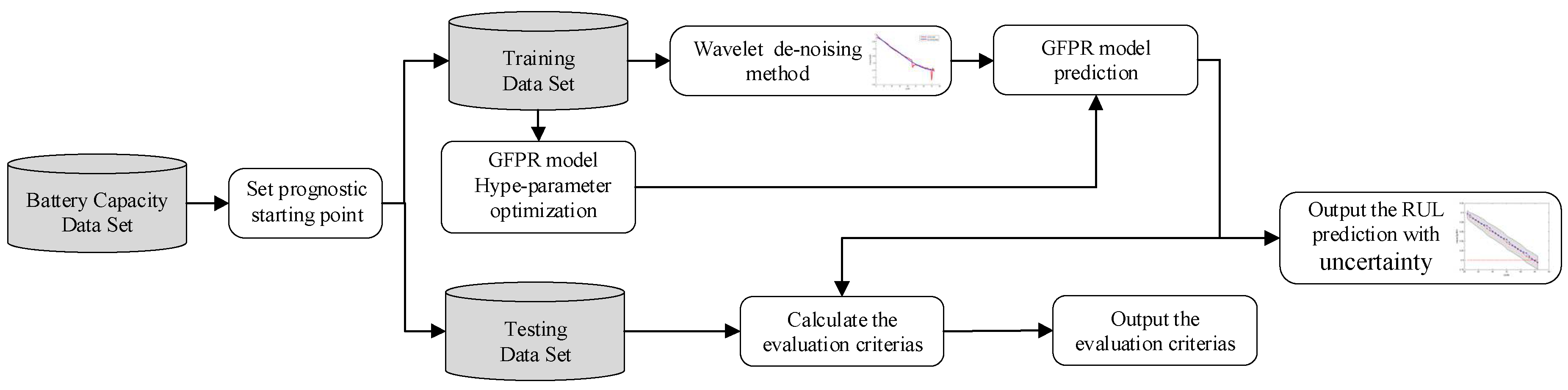
Depending on the station above, the flowchart for the proposed hybrid method for the battery RUL prognostics is shown in the Figure 1.

According to Figure 1, the input of the hybrid method is the capacity, and the output is prognostic capacity degradation trajectory with 95% confidence bounds. Then, the evaluation is given with testing data set and prediction results through some criteria. The fusion method of WD method and HGPFR model for the noise de-noising and battery RUL prediction are introduced as follows.

Definition: Hype-parameter $\mathsf{\Theta }={[a,b,{\sigma }_{f_1}^2,{\sigma }_{f_2}^2,l_1,l_2,\omega ,]}^T$ is an important factor to be optimized. Prognostic starting point is set to $T$. $Data\_train(T)$ reflects the training data for the HGPFR model that consists of the history data ${\left\{Cap(i),i\right\}}_{i=1}^{T-1}$. $WD\_Data\_train(T)$ reflects the preprocessed training data for the HGPFR model that consist of the history data ${\left\{WD\_Cap(i),i\right\}}_{i=1}^{T-1}$. $N$ means the total cycle life number of each data set. The process of proposed method is stated as follows.

Firstly, wavelet function $\varphi (t)$, the value of soft threshold $\lambda$, and the decomposition levels are initialized. Based on that, the original data that are decomposed for $J$ levels are decided. At the same time, the detail coefficient $d_{j,n}$ is obtained. Then, the de-noised signals are reconstructed. Next, the hype-parameter and times of optimization are initialized, and they are optimized by the maximization of the log-likelihood method. The de-noised signals are input to the HGFPR model. Finally, the model outputs the prediction results, and the evaluation criteria is given to evaluate the performance of hybrid method.

For clarity, the hybrid method with WD method and HGPFR model can be summarized in Algorithm 1.

Algorithm 1. The hybrid method with WD method and HGPFR algorithm

(1) Initialization:

Select the wavelet function $\varphi (t)$, the value of soft threshold $\lambda$, and the decomposition levels $J$;

(2) Decomposition:

Decompose the ${\left\{Cap(i),i\right\}}_{i=1}^{T-1}$ for the $J$ levels and calculate the detail coefficient $d_{j,n}$ form 1 to $J$ levels with Equation (6);

(3) Wavelet reconstruction:

The signals ${\left\{WD\_Cap(i),i\right\}}_{i=1}^{T-1}$ are reconstructed with the value of soft threshold $\lambda$ and detail coefficient $d_{j,n}$ form 1 to $J$ levels by the Equations (6) and (8);

(4) Initialize the hype-parameter and times of optimization:

Initializing value of hype-parameter is set to ${\mathsf{\Theta }}_0={[a_0,b_0,{({\sigma }_{f_1}^2)}_0,{({\sigma }_{f_2}^2)}_0,l_1{}^0,l_2{}^0,{\omega }_0]}^T$, and the times of optimization are set to $N_{op}$;

(5) Optimized the hype-parameter

FOR I = 1, …$N_{op}$

Calculate the hype-parameter ${\mathsf{\Theta }}^i$ using Equation (9) with the reconstruct signal ${\left\{WD\_Cap(i),i\right\}}_{i=1}^{T-1}$

Update the value of hype-parameter with ${\mathsf{\Theta }}^i$

END FOR;

(6) Output the prediction result:

Input the reconstruct signal ${\left\{WD\_Cap(i),i\right\}}_{i=1}^{T-1}$ to the prognostic model, and then capacity degradation trajectory with the 95% confidence bounds is obtained;

(7) Prognostic result evaluation:

The evaluation is given with testing data set and prediction results through some criteria to evaluate the performance of hybrid method.

4. Experiments and Discussion

To evaluate the performance of hybrid method, the lithium-ion battery data set is applied. The data set is characterized with different experiment conditions. The varieties of data set guarantee the adaptability and effectiveness of proposed model. Next, the detailed information and evaluation criteria will be introduced.

4.1. Raw Data from Lithium-Ion Battery and Evaluation Criteria

4.1.1. DES Lithium-Ion Battery Data Set

This section shows an overview of the raw data of the experiment. The data for carrying out the prediction model is from the DES, University of Oxford. The Bio-Logic MPG-205 lithium-ion battery systems are applied for the experiment of lithium-ion battery degradation. The test subject is the lithium-ion battery produced by the Kokam CO LTD [38,39,40]. The version of battery is SLPB533459H4 whose rated capacity is 740 mAh. Structures of the test data are made up of 5 kinds of forms consisting of charge rate, discharge rate, temperature of battery, open circuit voltage, and capacity at temperature of 40 °C. The details of the experimental conditions for the battery are given as follows.

• The thermal chamber is set to 40 °C.
• The lithium-ion battery is charged under the constant current of 0.74 A condition until the voltage attained 4.2 V.
• The battery is discharged under the constant current of 0.74 A condition until the voltage fell to 2.7 V.
• The capacity data are recorded every 100 cycles of drive cycles.

The lithium-ion batteries are repeated charging and discharging cycles to achieve accelerated the aging process. The impedance measurements completed by the electrochemical impedance spectroscopy (EIS) provide the internal parameters of the battery during the aging process. These experiments are carried out with the accelerated aging pattern. The number of charge or discharge cycles will be more than the results of these experiments in the actual application. In the experiment of the Department of Engineering Science, University of Oxford, the experiments are ended when the charged capacity of the lithium-ion batteries reaches about 80% of the rated capacity (from 0.74 Ah to about 0.60 Ah).

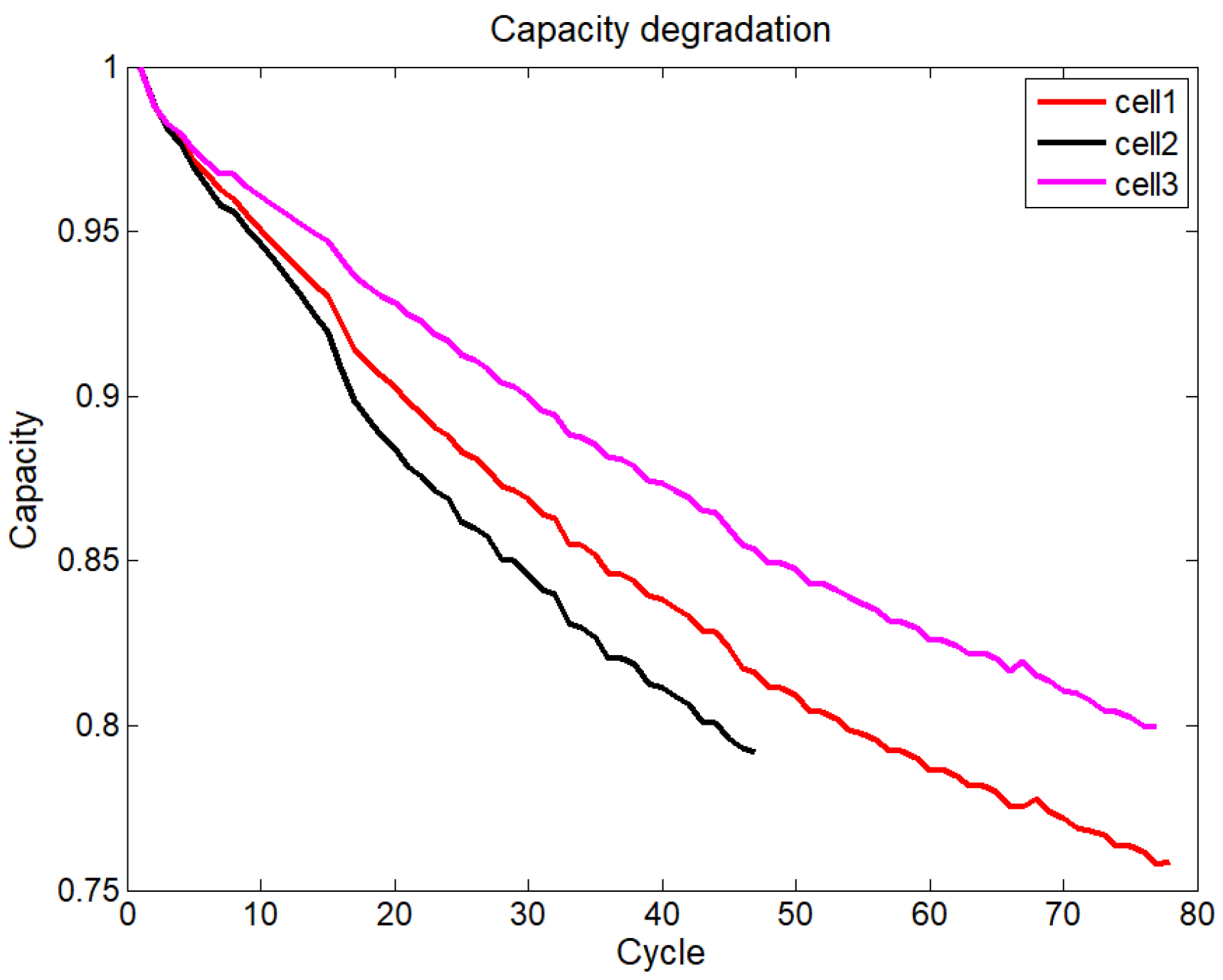
The data consist of training data and testing data for Cell-1, Cell-4, and Cell-7 batteries showing marked degradation characteristics through analyzing the data and experimental conditions. These sets of data are routine degradation performance test at temperature of 40 °C. Therefore, it is the representative for these sets of data to verify the method proposed in this paper. The results that measured the capacity of these data sets are shown in Figure 2. The measured capacity is normalized in this paper. For the reason that capacity data are recorded every 100 cycles of drive cycles, the values of horizontal ordinate are 100 times for the practical cycles. That means No. 10 cycle of the figures in this paper actually denotes No. 1000.

4.1.2. CALCE Lithium-Ion Battery Data Set

This section shows an overview of the raw data of the experiment. The data for carrying out the prediction model is from the CALCE, University of Maryland [41]. The Arbin BT2000 lithium-ion battery systems are applied for the experiment of lithium-ion battery degradation. To provide sufficient data, the data is divided into two parts with the difference of batteries’ rated capacity that is 1.35 Ah and 1.1 Ah for batteries, respectively, and the battery with 1.1 Ah rated capacity is chosen for the experiment. Structures of the data are made up of 3 kinds of forms (charge, discharge, and capacity) at room temperature. The details of the experimental conditions for the battery are shown as follows:

• The thermal chamber was set to 20 °C–25 °C.
• The lithium-ion battery was charged under the constant current of 0.55 A condition until the voltage attained 4.2 V.
• The battery was discharged under the constant current of 1.1 A condition until the voltage fell to 2.7 V.

The lithium-ion batteries are repeated charging and discharging cycles to achieve accelerated the aging process. The impedance measurements completed by the electrochemical impedance spectroscopy (EIS) provide the internal parameters of the battery during the aging process. That completed the progress of the lithium-ion batteries aging process. These experiments are carried out with the accelerated aging pattern. However, the number of charge or discharge cycle will be more than the results of these experiment in the actual application. In the experiment of the CALCE, the experiments are ended when the charged capacity of the lithium-ion batteries reaches about 80% of the rated capacity (from 1.1 Ah to about 0.88 Ah).

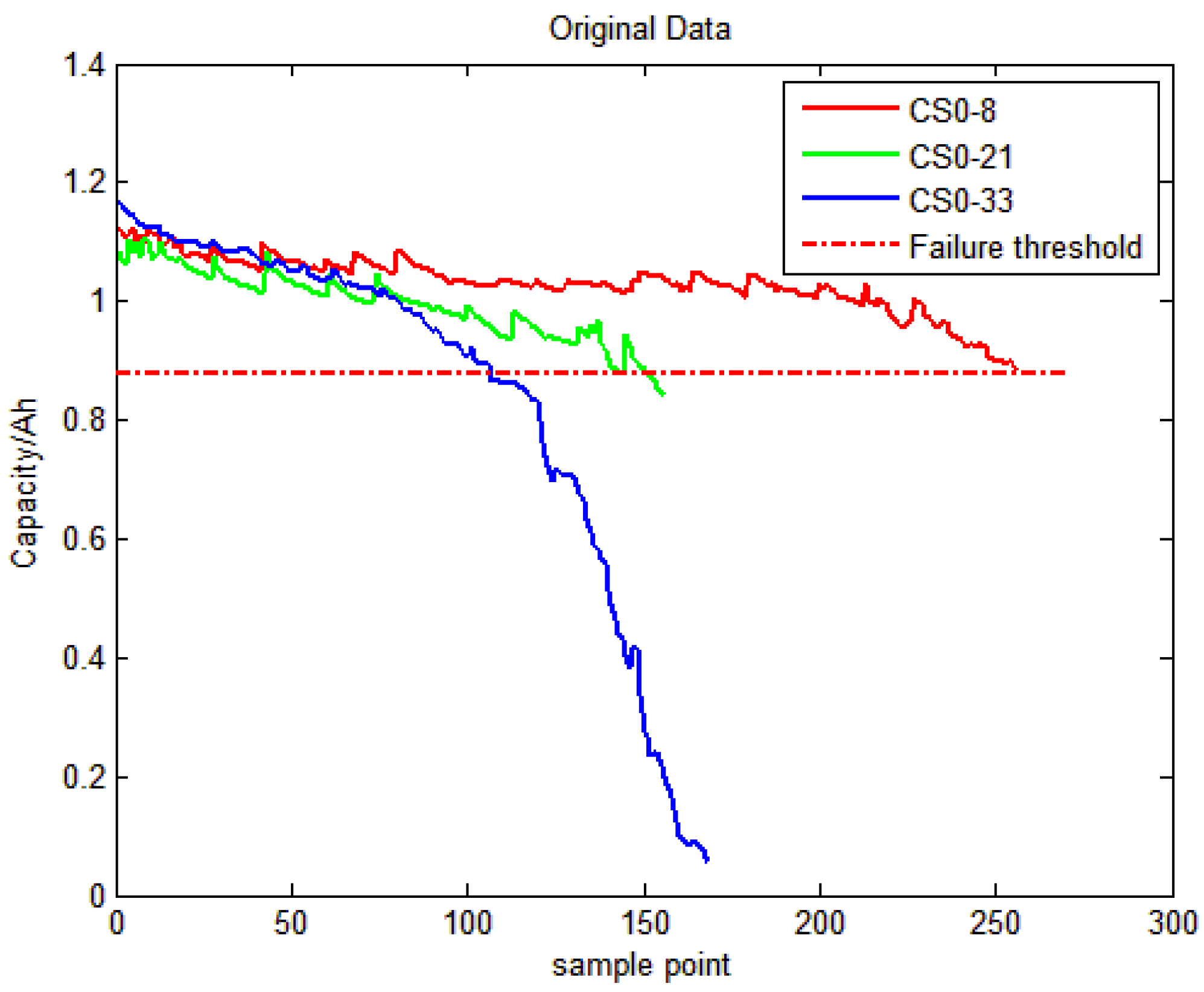
The data consists of training data and testing data for CS2-8, CS2-21, and CS2-33 batteries showing marked degradation characteristics through analyzing the data and experimental conditions. These sets of data are routine degradation performance test at room temperature, while the other batteries are accelerated aging experiments. Therefore, it is the representative for these sets of data to verify the method proposed in this paper. The results of the measured capacity of these sets of data are shown in Figure 3.

4.1.3. Evaluation Criteria

To validate the proposed model, four different evaluation criteria are used. They are shown as follows:

• SNR. It evaluates the performance of de-noising. The detailed information is shown as follows:

  $$SNR=10\lg \left[\frac{{\displaystyle \sum _{i=1}^n{(y_i)}^2}}{{\displaystyle \sum _{i=1}^n{(y_i-{\widehat{y}}_i)}^2}}\right]$$

  (23)
• Err: relative error of RUL prediction. The detailed information is shown as follows:

  $$RUL\_err=\left|\frac{{\widehat{y}}_{RUL}-y_{RUL}}{y_{RUL}}\right|$$

  (24)
• RMES reflects the root mean squared error. The detailed information is shown as follows:

  $$RMES({\widehat{y}}_i,y_i)=\sqrt{\frac{{\displaystyle {\sum }_{i=1}^n{(y_i-{\widehat{y}}_i)}^2}}{n}}$$

  (25)
• MAPE means absolute percentage error. The detailed information is shown as follows:

  $$MAPE({\widehat{y}}_i,y_i)=\frac{1}{n}{\displaystyle \sum _{i=1}^n\left|\frac{y_i-{\widehat{y}}_i}{y_i}\right|}$$

  (26)

in which $y_i$ reflects the measured value and ${\widehat{y}}_i$ refers to the predicted value. $n$ is the number of raw data. ${\widehat{y}}_{RUL}$ and $y_{RUL}$ reflect the value of RUL prediction and the measured RUL value.

The evaluation criteria described above analyze the values between the prediction starting point and end of life (EOL), not only the value of EOL. Some problems can be avoided by this evaluation criteria. For example, the trajectory of prognostic model is far from the true trajectory, but the value of EOL prediction is closed to the EOL. That prognostic model is not good.

4.2. The Selection of Wavelet De-Noising Method

For the selection of wavelet de-noising method, there are three factors that affect the performance containing the value of threshold, wavelet basis, and decomposition levels. Next, the selection of these three factors will be analyzed.

4.2.1. The Selection of Threshold Value

The value of threshold is a vital part of the selection of wavelet de-noising method. It is a dividing line for removing the noise from useful signals. If the selections for threshold value are not suitable, the results processed by the wavelet de-noising method are unsatisfied. In general, the conventional threshold value is expressed as follows [42,43,44]:

$$\lambda =\sigma \sqrt{2\log (N)}$$

(27)

in which $\sigma$ reflects the standard deviation of interference noise. $N$ refers to the length of original data.

According to the wavelet theory, the wavelet factors will be decreased as the increase of decomposition levels. Hence, a constant threshold value is not suitable for practical application. To overcome this problem, reference [45,46] propose an adaptive threshold value shown as follows:

$$\lambda =\frac{\sigma \sqrt{2\log (N)}}{\log (J+1)}$$

(28)

in which $J$ reflects the decomposition levels. $N$ means the length of original data.

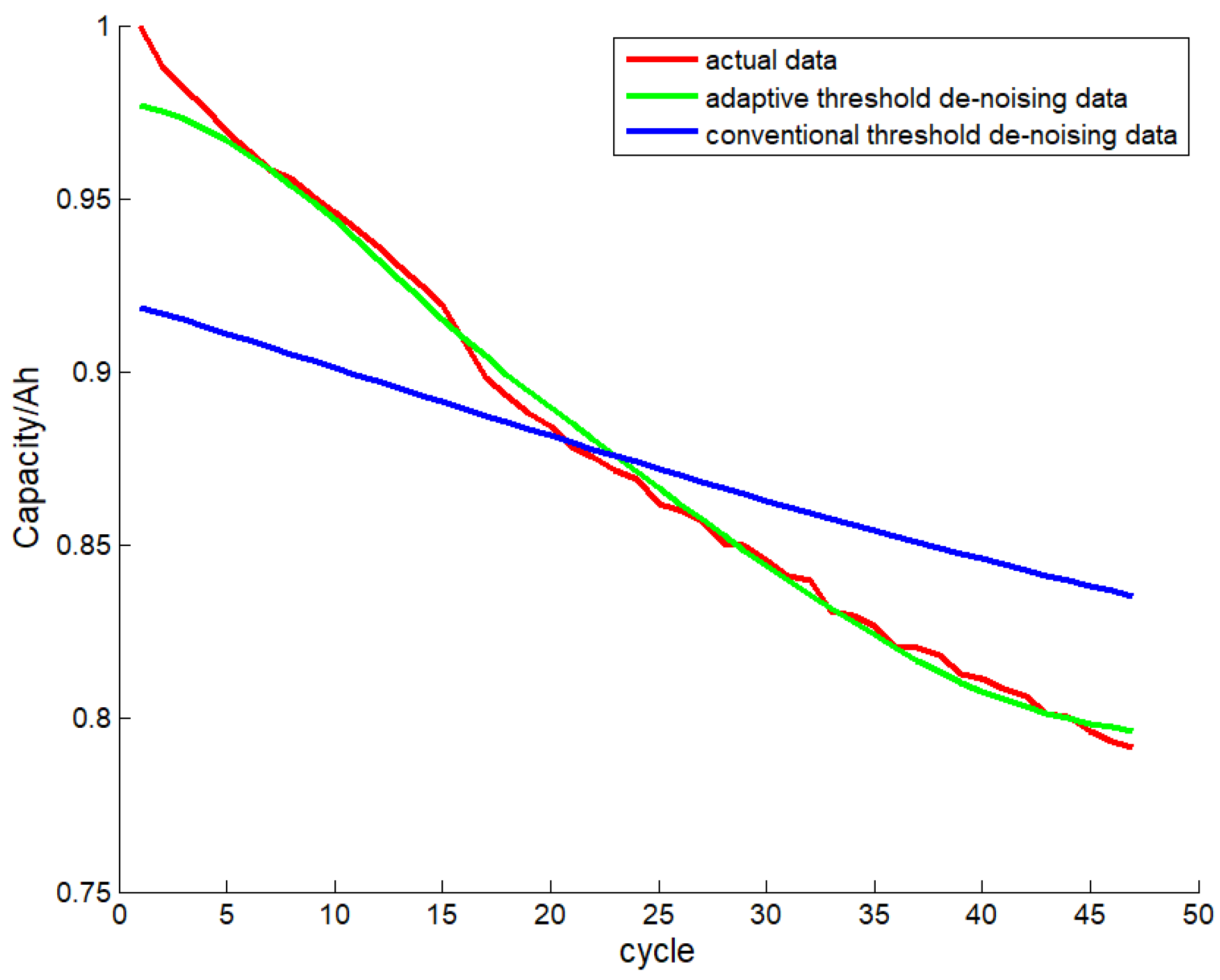
From Equation (29), we know that threshold values decrease as the decomposition levels that conform with the wavelet theory increase. Figure 4 shows the de-noised results through these 2 different threshold values by the 5th Symlets (sym5) wavelet basis with Cell-1 battery data.

In Figure 3, we know that the trend of trajectory processed by adaptive threshold value is better than the conventional ones. Furthermore, according to calculation, the SNR value of de-noised result with the conventional threshold value is 61.7144 dB, and the SNR value of de-noised result with the adaptive threshold value is 78.8679 dB. Thus, the performance of adaptive threshold value is higher than the conventional one’s. Therefore, in this study, the adaptive threshold value is chosen for the wavelet denoising method.

4.2.2. The Selection of Wavelet Basis and Decomposition Levels

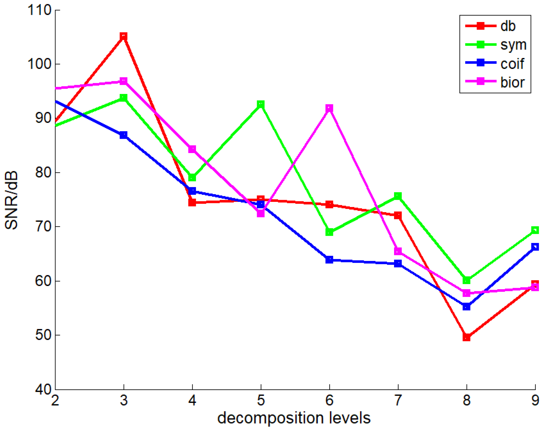
The wavelet basis is another important factor for selecting of wavelet denoising method. The type of wavelet function is specified by the wavelet basis essentially. To improve the performance, it is essential to select a suitable wavelet basis. Generally speaking, there are four factors affecting wavelet basis consisting of orthogonality, symmetry, compact support, regularity, and vanishing moments. Hence, to achieve the appreciated wavelet basis, Symlets (sym)wavelet base, Daubechies (db)wavelet base, Coiflets (coif)wavelet base, and Biorthogonal (bior)wavelet base are applied to de-noise the battery data. In this paper, the decomposition levels are chosen from 2 to 9. The de-noised results for these four wavelet bases with Cell-1 battery data are shown in Figure 4.

In Figure 5, we know that all these four trajectories are characterized by the tendency from rise to decline. While the decomposition is set to be 3, the SNR value of db wavelet base is the maximum. Thus, the db wavelet base is chosen as the wavelet basis.

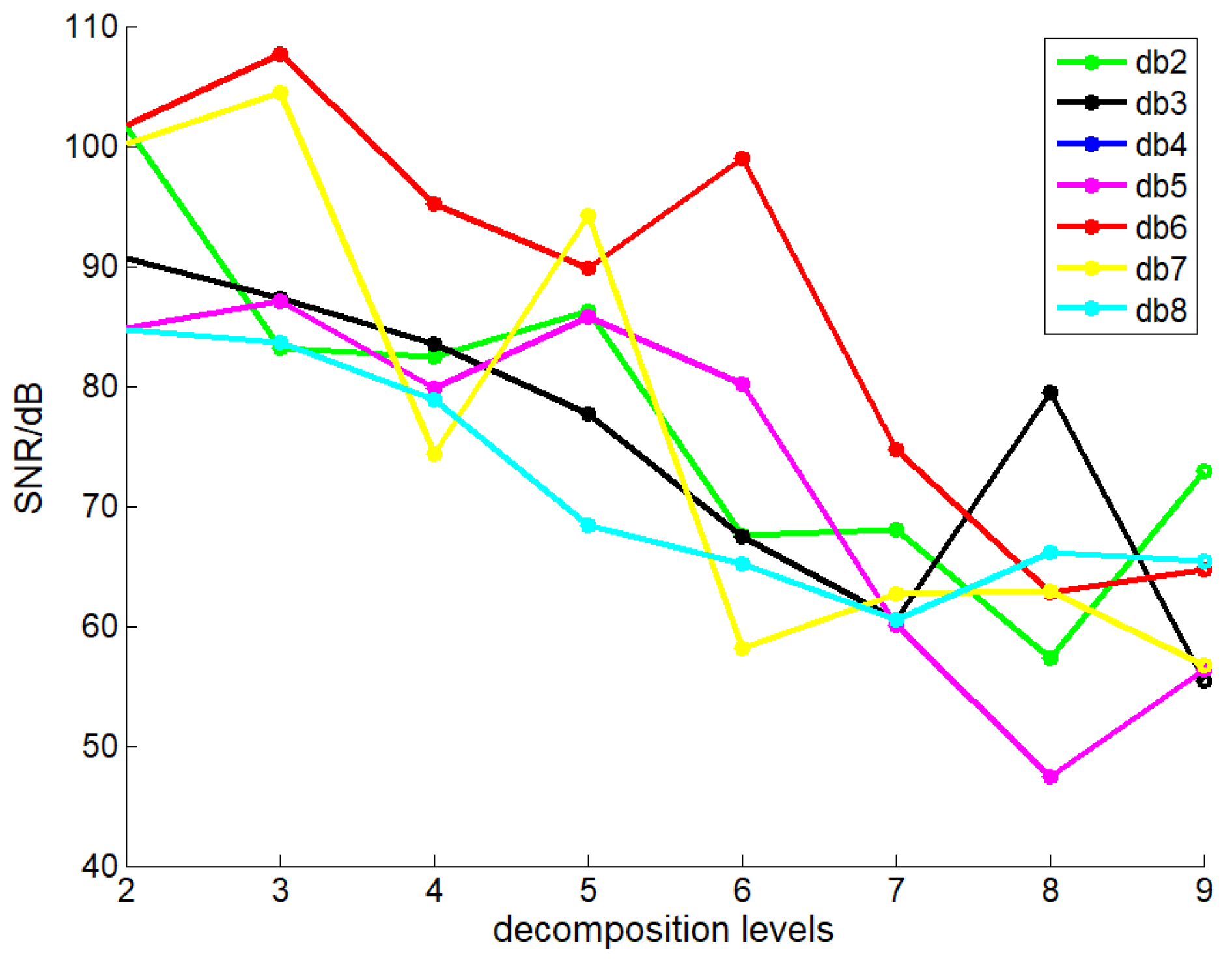
For the detailed selection information of db wavelet base, the db2 to db9 is simulated from 2 to 8 decomposition levels. The simulation consequence with Cell-1 battery data of DES is given in the Figure 6.

In Figure 6, we know that while the decomposition levels are less than 7, the trajectory of db6 wavelet basis nearly outstrips others. Therefore, the db6 is chosen as the wavelet base for wavelet de-noising method.

4.3. Battery RUL Prognostics with Hybrid Method

This part is organized as follows. First, the performances of proposed hybrid method are compared with the HGFPR model and GPR model. Then, the performance of proposed hybrid method is evaluated. The experiments of evaluation are carried out by the lithium-ion battery data sets provided by DES and CALCE, respectively. To evaluate the prognostic results, the evaluation criteria are calculated with the original data and prognostic results.

4.3.1. DES Lithium-Ion Battery RUL Prediction Result

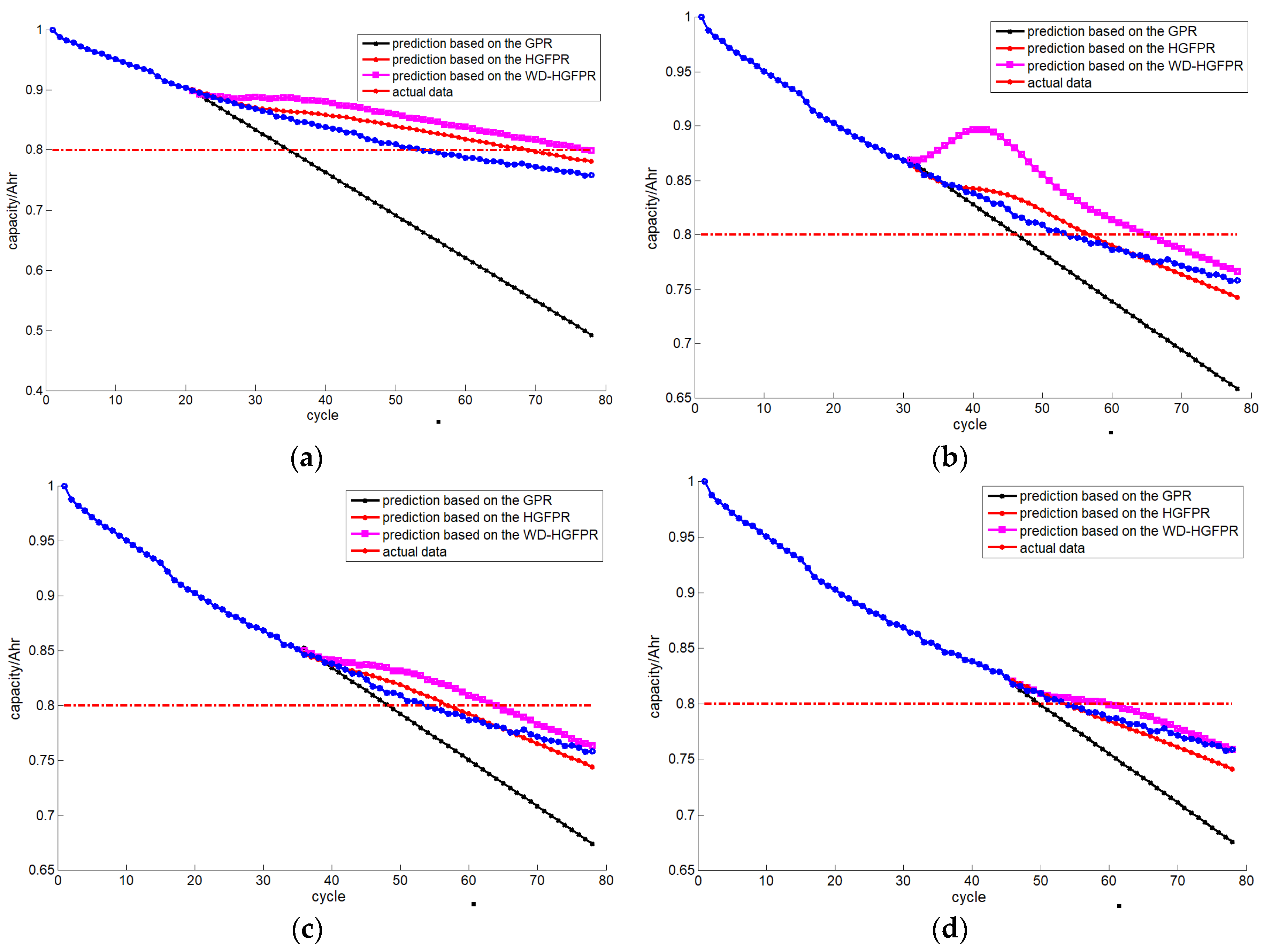
To clarify the performances with different models clearly, the Cell-1 battery data are applied, and the lengths of training data are set to be 20, 30, 35, and 45, respectively. Figure 7 shows the prediction results using three different models with different lengths of training data for Cell-1 battery.

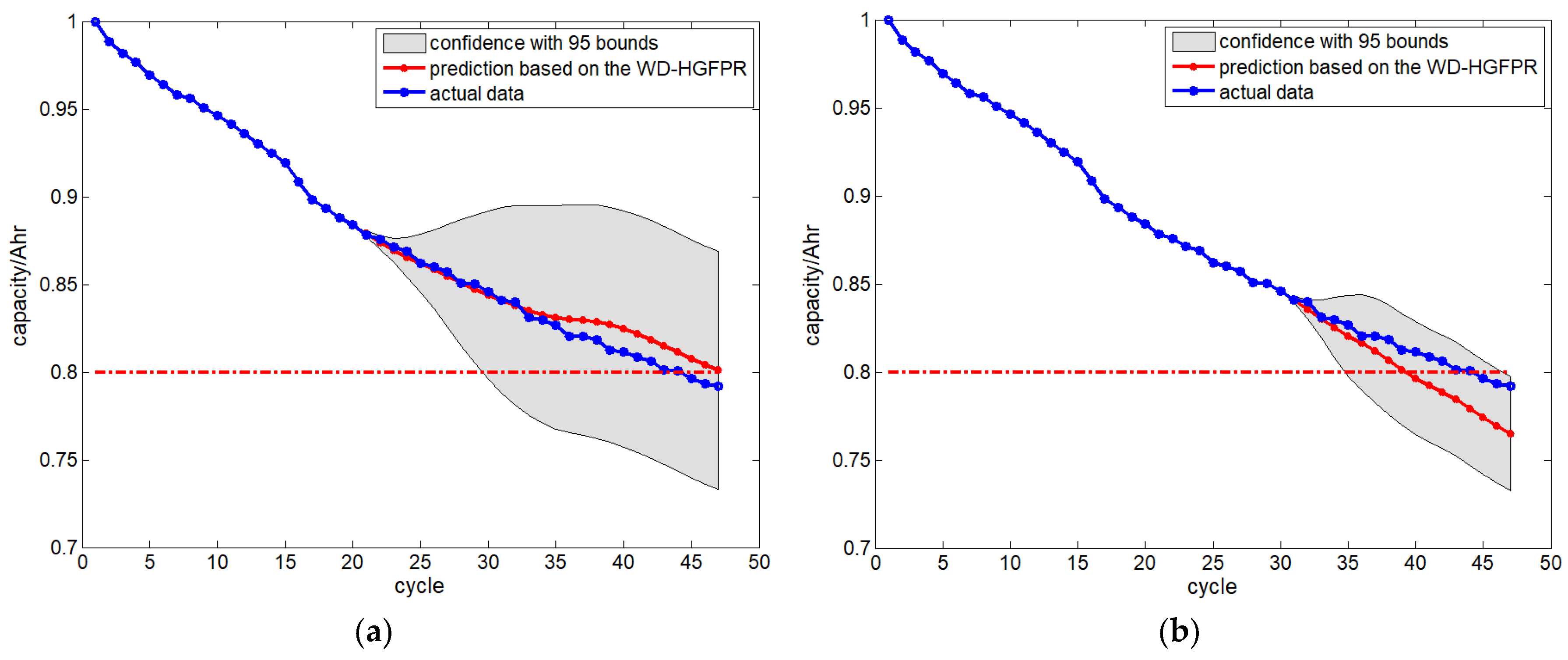
In Figure 7, it can be seen that, under the condition in which the length of training data and the same initialization of hype-parameter are the same, the performance of RUL prognostic results and trajectory fitting tendency processed by the proposed method are better than the HGFPR model and GPR model. The prognostic results for the rest of other two battery data set with 95% confidence are shown as Figure 8 and Figure 9.

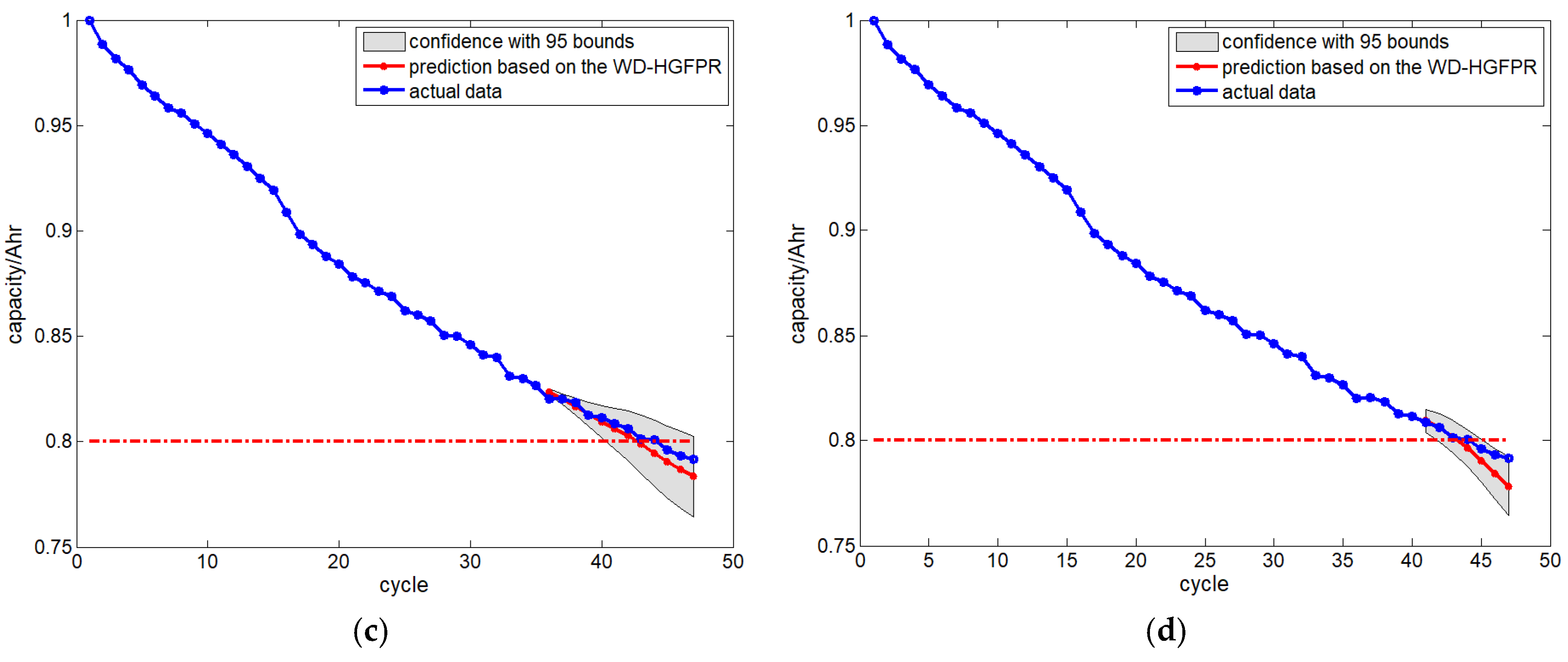
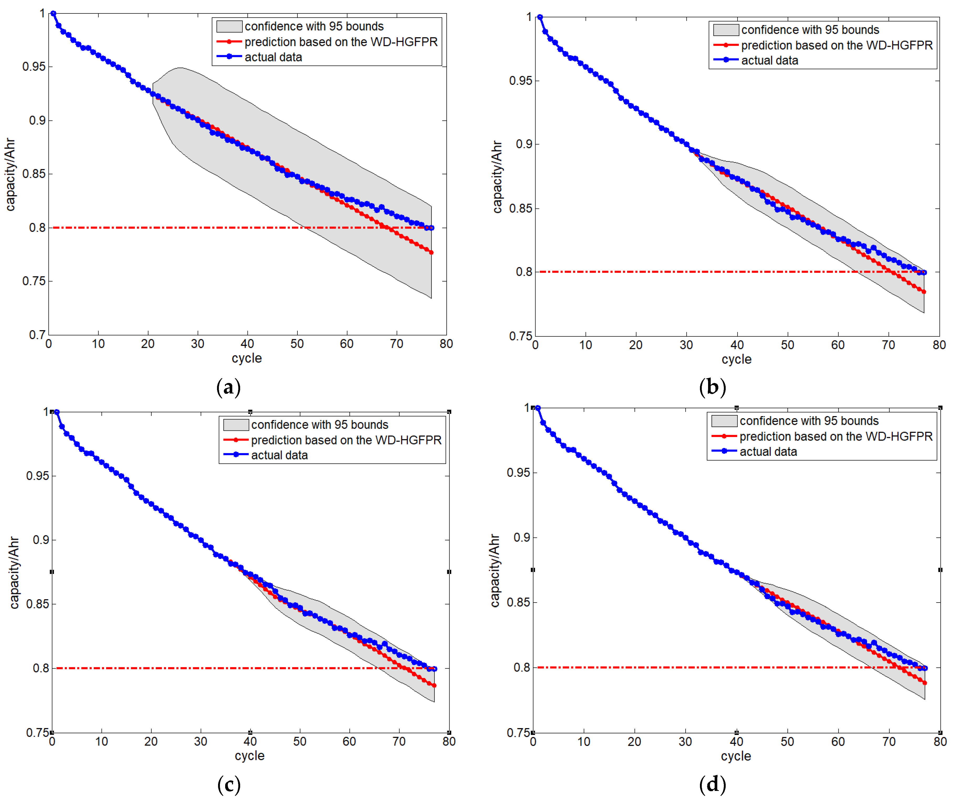
As is shown in Figure 8 and Figure 9, it can be seen that the prognostic results are better with more training data.

Table 1. Prognostic results and evaluation criteria using different methods with different lengths of training data.

Data Set	Start Point	WD-HGPFR			HGPFR			GPR
		Err	RMSE	MAPE	Err	RMSE	MAPE	Err	RMSE	MAPE
C-1	20	25.0%	0.0236	0.0253	32.2%	0.0406	0.0444	37.7%	0.1589	0.2319
	30	8.9%	0.0108	0.0103	23.2%	0.0408	0.0438	17.0%	0.0600	0.0720
	35	5.4%	0.0072	0.0075	17.9%	0.0181	0.0167	13.2%	0.0525	0.0632
	40	3.6%	0.0108	0.0099	7.3%	0.0163	0.0181	9.4%	0.0598	0.0767
C-4	20	6.7%	0.0079	0.0076	20.0%	0.0600	0.0645	24.4%	0.0984	0.1035
	30	11.1%	0.0509	0.0639	15.6%	0.0772	0.0901	20.0%	0.0893	0.0907
	35	4.4%	0.0044	0.0046	15.6%	0.0053	0.0055	17.8%	0.0482	0.0578
	40	2.2%	0.0026	0.0026	6.7%	0.0028	0.0037	11.1%	0.0364	0.0471
C-7	20	10.9%	0.0273	0.0289	16.0%	0.0354	0.0433	21.0%	0.1305	0.1437
	30	6.7%	0.0061	0.0126	12.0%	0.0147	0.0141	17.1%	0.1026	0.1147
	35	5.3%	0.0056	0.0050	9.3%	0.0444	0.0465	13.2%	0.0833	0.0945
	40	2.7%	0.0145	0.0169	5.3%	0.0231	0.0248	10.5%	0.0681	0.0842

lists the prognostic results and evaluation criteria by HGPFR methods and GPR model with different length of training data.

Firstly, as is shown in Table 1, it can be seen that most predictions of relative errors are less than 7%. Furthermore, for the evaluation criteria, the proposed model can achieve smaller values of RMSE and MAPE than HGFPR model and GPR model. This means that the proposed model in this paper can achieve satisfied prediction accuracy. Besides, the error can be reduced when the ending point of training data is closer to the EOL point for the two different models. This refers to the fact that more training data can help improve the accuracy of prediction. Unfortunately, according to the prognostic results, the highest relative error arises in the Cell-1 battery with 20 training data. This phenomenon may occur for two reasons. On the one hand, the training data are so few that the optimized hype-parameter cannot be obtained. On the other hand, the degradation trajectory appears to have larger tendency changes near the 20th point that are inconsistent with the following degradation trend. This may cause the parameters to change for the log-likelihood algorithm. Thus, proposed method may lose the prediction performance.

Secondly, the Cell-4 obtains the most accurate prediction result compared with other 2 cells battery data. However, the Cell-1 are performed with the worst prediction result. The reason for this is that the data size of Cell-4 is smaller than other 2 cells, and the proportion is higher than the same number of training data. That means the hype-parameter is optimized better than other 2 cells. The other reason is that the relative degradation tendency of Cell-1 is larger than other 2 cells, and the optimized hype-parameter cannot be obtained. Nevertheless, with the increase of training data, the prediction accuracy of Cell-1 is higher, and the highest accuracy is 3.6%, which is acceptable. Despite the fact that the prediction accuracy is not satisfactory at one test point, an acceptable RUL prediction can be still achieved using the proposed method.

4.3.2. CALCE Lithium-Ion Battery RUL Prediction Result

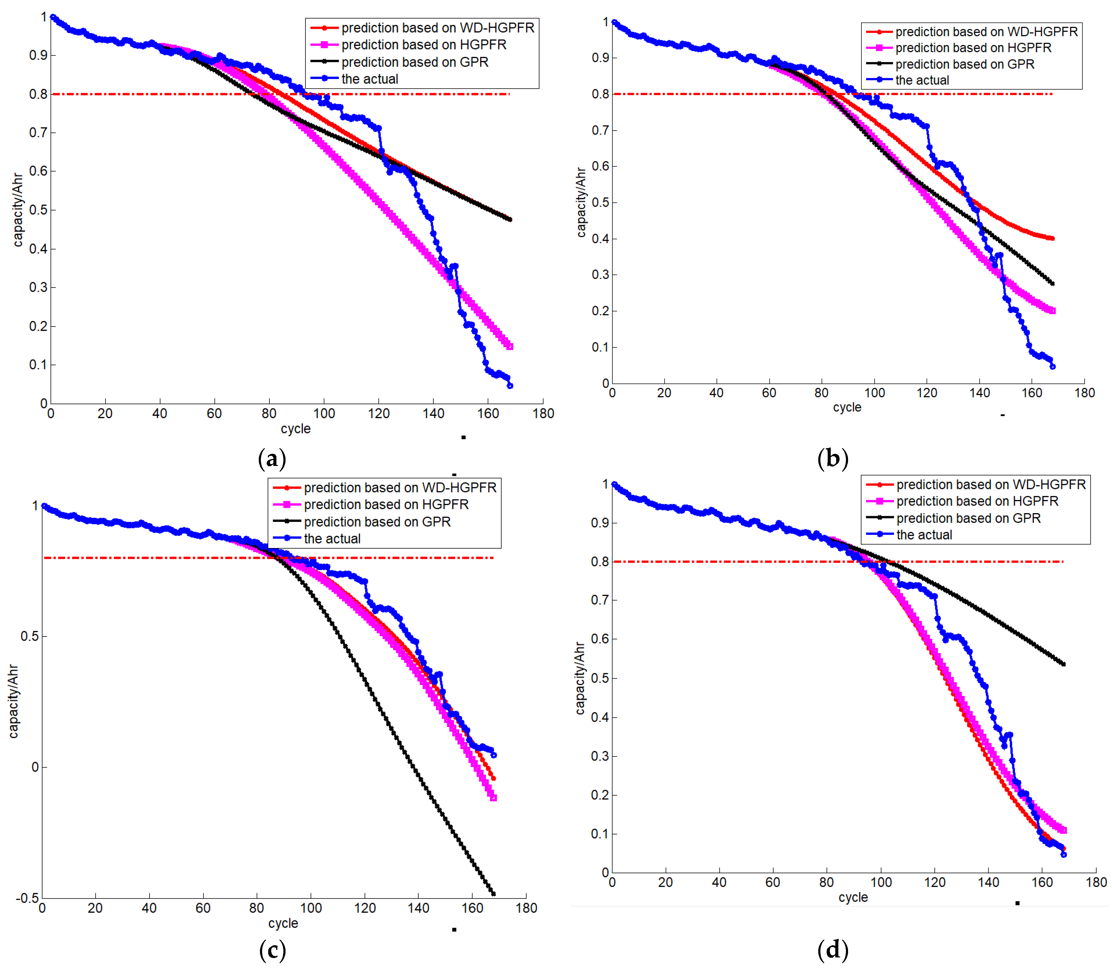
To clarify the performances with different model clearly, the Cell-33 battery data are applied, and the lengths of training data are set to 40, 60, 70, and 80, respectively. Figure 10 shows the prediction results using three different models with different lengths of training data for Cell-33 battery.

In Figure 10, it can be seen that, under the condition in which the length of training data and the same initialization of hype-parameter are the same, the performance of RUL prognostic results and trajectory fitting tendency processed by the proposed method are better than the HGFPR model and GPR model.

Table 2. Prognostic results and evaluation criteria using different methods with different lengths of training data.

Data Set	Start Point	WD-HGPFR			HGPFR			GPR
		Err	RMSE	MAPE	Err	RMSE	MAPE	Err	RMSE	MAPE
C-8	150	11.9%	0.0979	0.1036	14.2%	0.3980	0.4746	17.9%	0.4058	0.5318
	180	9.1%	0.0817	0.0952	9.9%	0.1935	0.2579	11.5%	0.3368	0.4238
	210	7.1%	0.0774	0.0853	8.7%	0.1309	0.1537	10.3%	0.2088	0.2607
	230	4.7%	0.0895	0.1299	6.3%	0.1371	0.1625	7.5%	0.1366	0.1452
C-21	70	9.7%	0.1363	0.1428	12.3%	0.1784	0.1908	14.2%	0.2355	0.3087
	90	7.8%	0.0933	0.1132	9.9%	0.1012	0.1398	10.4%	0.1177	0.1736
	110	6.4%	0.0767	0.0973	7.8%	0.0907	0.1124	11.0%	0.1325	0.2038
	130	5.2%	0.0663	0.0909	5.8%	0.0832	0.0922	7.2%	0.0912	0.1331
C-33	40	8.6%	0.0784	0.1637	15.1%	0.0947	0.1340	20.4%	0.1637	0.1921
	60	7.5%	0.0817	0.1053	12.9%	0.0992	0.1340	11.8%	0.1184	0.2191
	70	5.3%	0.0245	0.0369	7.5%	0.0463	0.0576	8.6%	0.3391	0.4790
	80	3.2%	0.0863	0.1989	4.3%	0.0954	0.2129	10.7%	0.2373	0.2717

lists other two battery cells prognostic results and evaluation criteria using HGPFR methods and GPR model with different lengths of training data. For the different end of life, the length of training is different.

As is shown in Table 2, it can be seen that the proposed model can achieve smaller values of RMSE and MAPE than HGFPR model and GPR model. This means that the proposed model in this paper can get a satisfied prediction accuracy. However, the Cell-8 is performed with the worst prediction result. The reason for this may be the fact that degradation trajectory of Cell-8 changes more than other two cells, so the optimized hype-parameter cannot be obtained. Nevertheless, with the increase of training data, the prediction accuracy of Cell-33 is higher, and the highest accuracy is 3.2%, which is acceptable. The proposed method can also perform well with lithium-ion battery data sets under different work conditions.

5. Conclusions

This paper tries to improve the performance for RUL prognostics of lithium-ion battery through the domain transformation model and the data-driven method. A fusion method of the WD method and the HGPFR model is proposed to remove the noise from the original data and obtain a higher accuracy RUL prediction. Contributions to this paper can be summarized in the following three terms: (1) To reduce the impact of noise and obtain higher accuracy RUL prediction results, the WD method is applied. (2) In consideration of the degradation characteristics of the lithium-ion battery data set, the selection of the wavelet de-noising method is performed with corresponding experiments analyses. This method can remove the noise form useful data effectively. Furthermore, the key features are also distilled. This guarantees the significance of the de-noise data. (3) The hybrid method obtained RUL prediction results with 95% confidence bounds, producing profound value with practical applications.

The data for carrying out the prediction model is from the DES and CALCE. It is representative of these sets of data to that are used to verify the method proposed in this paper. With different cells degradation data, the proposed method performed satisfactorily. Most of the predictions of relative errors are less than 7%. Furthermore, for the evaluation criteria, the proposed model can achieve smaller values of RMSE and MAPE than the HGFPR model. This means that the proposed model in this paper can achieve satisfied prediction accuracy. What is more, the hybrid method has features that express the confidence bounds during the prediction.

In the future, the update of the hybrid method is considered for the wider application and higher accuracy. The present WD-HGPFR method shows the satisfied performance with RUL prediction for the specific condition. Hence, it is meaningful to discover a method that updates the WD-HGPFR model as the prediction process functions for RUL prediction on dynamic conditions. At the same time, it is useful to compare the proposed approach with existing ones, such as RVM, EKF, etc. This will make sense of the wider applications and higher accuracy of the model.

References

- Song, Y.; Liu, D.; Hou, Y.; Peng, Y. Satellite lithium-ion battery remaining useful life estimation with an iterative updated RVM fused with the KF algorithm. Chin. J. Aeronaut. 2018, 31, 31–40. [Google Scholar] [CrossRef]
- Song, Y.; Liu, D.; Yang, C.; Peng, Y. Data-driven hybrid remaining useful life estimation approach for spacecraft lithium-ion battery. Microelectron. Reliab. 2017, 75, 142–153. [Google Scholar] [CrossRef]
- Liu, D.; Zhou, J.; Pan, D.; Peng, Y.; Peng, X. Lithium-ion battery remaining useful life estimation with an optimized Relevance Vector Machine algorithm with incremental learning. Measurement 2015, 63, 143–151. [Google Scholar] [CrossRef]
- Dalal, M.; Ma, J.; He, D. Lithium-ion battery life prognostic health management system using particle filtering framework. J. Risk Reliab. 2015, 225, 81–90. [Google Scholar] [CrossRef]
- Zhang, Y.; Xiong, R.; He, H. Evaluation of the model-based state-of-charge estimation methods for lithium-ion batteries. In Proceedings of the 2016 IEEE Transportation Electrification Conference and Expo (ITEC), Dearborn, MI, USA, 26–29 June 2016; pp. 1–8. [Google Scholar]
- Liu, D.; Zhou, J.; Liao, H.; Peng, Y.; Peng, X. A health indicator extraction and optimization framework for lithium-ion battery degradation modeling and prognostics. IEEE Trans. Syst. Man Cybern. Syst. 2015, 45, 915–928. [Google Scholar]
- Zhang, H.; Miao, Q.; Zhang, X.; Liu, Z. An improved unscented particle filter approach for lithium-ion battery remaining useful life prediction. Microelectron. Reliab. 2018, 81, 288–298. [Google Scholar] [CrossRef]
- Wei, Z.; Zou, C.; Leng, F.; Soong, B.H.; Tseng, K.J. Online model identification and state of charge estimate for lithium-ion battery with a recursive total least squares-based observer. IEEE Trans. Ind. Electron. 2018, 65, 1336–1346. [Google Scholar] [CrossRef]
- Zou, C.; Hu, X.; Wei, Z.; Tang, X. Electrothermal dynamics-conscious lithium-ion battery cell-level charging management via state-monitored predictive control. Energy 2017, 141, 250–259. [Google Scholar] [CrossRef]
- Lin, C.; Yu, Q.; Xiong, R.; Wang, L. A study on the impact of open circuit voltage tests on state of charge estimation for lithium-ion batteries. Appl. Energy 2017, 205, 892–902. [Google Scholar] [CrossRef]
- Zou, C.; Hu, X.; Wei, Z.; Wik, T.; Bo, E. Electrochemical estimation and control for lithium-ion battery health-aware fast charging. IEEE Trans. Ind. Electron. 2017, 65, 6635–6645. [Google Scholar] [CrossRef]
- Hu, X.; Li, S.; Peng, H. A comparative study of equivalent circuit models for Li-ion batteries. J. Power Sources 2012, 198, 359–367. [Google Scholar] [CrossRef]
- Lai, X.; Zheng, Y.; Sun, T. A comparative study of different equivalent circuit models for estimating state-of-charge of lithium-ion batteries. Electrochim. Acta 2017, 259, 566–577. [Google Scholar] [CrossRef]
- Skoog, S.; David, S. Parameterization of linear equivalent circuit models over wide temperature and SOC spans for automotive lithium-ion cells using electrochemical impedance spectroscopy. J. Energy Storage 2017, 14, 39–48. [Google Scholar] [CrossRef]
- Xiong, R.; Tian, J.; Mu, H.; Wang, C. A systematic model-based degradation behavior recognition and health monitoring method for lithium-ion batteries. Appl. Energy 2017, 207, 372–383. [Google Scholar] [CrossRef]
- Hu, C.; Jain, G.; Schmidt, C.; Strief, C.; Sullivan, M. Online estimation of lithium-ion battery capacity using sparse bayesian learning. J. Power Sources 2015, 289, 105–113. [Google Scholar] [CrossRef]
- Zou, C.; Manzie, C.; Nešić, D.; Kallapur, A.G. Multi-time-scale observer design for state-of-charge and state-of-health of a lithium-ion battery. J. Power Sources 2016, 335, 121–130. [Google Scholar] [CrossRef]
- Wei, Z.; Meng, S.; Tseng, K.J.; Lim, T.; Soong, H.; Skyllas-Kazacos, M. An adaptive model for vanadium redox flow battery and its application for online peak power estimation. J. Power Sources 2017, 344, 195–207. [Google Scholar] [CrossRef]
- Liu, D.; Luo, Y.; Peng, Y.; Peng, X.; Pecht, M. Lithium-ion battery remaining useful life estimation based on nonlinear ar model combined with degradation feature. In Proceedings of the Annual Conference of the Prognostics and Health Management Society, Minneapolis, MN, USA, 23–27 September 2012; Volume 3, pp. 1803–1836. [Google Scholar]
- Zhang, J.; Lee, J. A review on prognostics and health monitoring of Li-ion battery. J. Power Sources 2011, 196, 6007–6014. [Google Scholar] [CrossRef]
- Liu, D.; Wang, H.; Peng, Y.; Xie, W.; Liao, H. Satellite lithium-ion battery remaining cycle life prediction with novel indirect health indicator extractcion. Energies 2013, 6, 3654–3668. [Google Scholar] [CrossRef]
- Saha, B.; Goebel, K. Uncertainty management for diagnostics and prognostics of batteries using Bayesian techniques. In Proceedings of the IEEE Aerospace Conference, Big Sky, MT, USA, 1–8 March 2008; pp. 1–8. [Google Scholar]
- Hu, C.; Jain, G.; Tamirisa, P.; Gorka, T. Method for estimating capacity and predicting remaining useful life of lithium-ion battery. Appl. Energy 2014, 126, 182–189. [Google Scholar] [CrossRef]
- Sun, P.; Wang, Z. Research of the relationship between Li-ion battery charge performance and SOH based on miga-gpr method. Energy Procedia 2016, 88, 608–613. [Google Scholar]
- Li, F.; Xu, J. A new prognostics method for state of health estimation of lithium-ion batteries based on a mixture of Gaussian process models and particle filter. Microelectron. Reliab. 2015, 55, 1035–1045. [Google Scholar] [CrossRef]
- Liu, D.; Pang, J.; Zhou, J.; Peng, Y.; Pecht, M. Prognostics for state of health estimation of lithium-ion batteries based on combination Gaussian process functional regression. Microelectron. Reliab. 2013, 53, 832–839. [Google Scholar] [CrossRef]
- Wang, D.; Miao, Q. Smoothness index-guided bayesian inference for determining joint posterior probability distributions of anti-symmetric real laplace wavelet parameters for identification of different bearing faults. J. Sound Vib. 2015, 345, 250–266. [Google Scholar] [CrossRef]
- Diop, M.; Wright, E.; Toronov, V.; Lee, T. Improved light collection and wavelet de-noising enable quantification of cerebral blood flow and oxygen metabolism by a low-cost, off-the-shelf spectrometer. J. Biomed. Opt. 2014, 19, 57007. [Google Scholar] [CrossRef] [PubMed]
- Juš, K.; Tanko, V. Prognosis of gear health using Gaussian process model. In Proceedings of the IEEE Eurocon—International Conference on Computer as a Tool, Lisabon, Portugal, 27–29 April 2011; pp. 1–4. [Google Scholar]
- Rasmussen, C.E.; Williams, C.K.I. Gaussian Processes for Machine Learning; MIT Press: Cambridge, MA, USA, 2006. [Google Scholar]
- MacKay, D. Introduction to Gaussian Processes; Technical Report; Cambridge University: Cambridge, UK, 1997; Available online: http://wol.ra.phy.cam.ac.uk/mackay/README.html (accessed on 3 May 2018).
- Shi, J.Q.; Wang, B. Gaussian process functional regression modeling for batch data. Biometrics 2007, 63, 14–23. [Google Scholar] [CrossRef] [PubMed]
- Williard, N.; He, W.; Hendricks, C.; Pecht, M. Lessons learned from the 787 dreamliner issue on lithium-ion battery reliability. Energies 2013, 6, 4682–4695. [Google Scholar] [CrossRef]
- Williams, C.K.I.; Rasmussen, C.E. Gaussian processes for regression. In Advances in Neural Information Processing Systems 8; David, S.T., Michael, C.M., Michael, E.H., Eds.; MIT Press: Cambridge, MA, USA, 1996. [Google Scholar]
- Tao, C.; Julian, M.; Elaine, M. Gaussian process regression for multivariate spectroscopic calibration. Chem. Intell. Lab. Syst. 2007, 87, 59–71. [Google Scholar] [Green Version]
- Yunong, Z.; Leithead, W.E.; Leith, D.J. Time-series Gaussian process regression based on toeplitz computation of O(N2) operations and O(N)-level storage. In Proceedings of the 2005 European Control Conference on Decision and Control, Seville, Spain, 12–15 December 2005; pp. 3711–3716. [Google Scholar]
- Girard, A.; Murraysmith, R. Gaussian processes: Prediction at a noisy input and application to iterative multiple-step ahead forecasting of time-series. Lect. Notes Comput. Sci. 2003, 3355, 158–184. [Google Scholar]
- Christoph, R.B. Diagnosis and Prognosis of Degradation in Lithium-Ion Batteries. Ph.D. Thesis, Department of Engineering Science, University of Oxford, Oxford, UK, 2017. [Google Scholar]
- Birkl, C. Oxford Battery Degradation Dataset 1; University of Oxford: Oxford, UK, 2017. [Google Scholar]
- Fyfe, R.; Zuo, J.; Lin, J. Mechanical fault detection based on the wavelet de-noising technique. J. Vib. Acoust. 2004, 126, 9–16. [Google Scholar]
- Pecht, M.; Jaai, R. A prognostics and health management roadmap for information and electronics-rich systems. Microelectron. Reliab. 2010, 50, 317–323. [Google Scholar] [CrossRef]
- Liao, Y.; Fan, Y.; Cheng, F. On-line prediction of pH values in fresh pork using visible/near-infrared spectroscopy with wavelet de-noising and variable selection methods. J. Food Eng. 2012, 109, 668–675. [Google Scholar] [CrossRef]
- Bachner-Hinenzon, N.; Ertracht, O.; Lysiansky, M.; Binah, O.; Adam, D. Layer-specific assessment of left ventricular function by utilizing wavelet de-noising: A validation study. Med. Biol. Eng. Comput. 2011, 49, 3–13. [Google Scholar] [CrossRef] [PubMed]
- Chen, Y.; Miao, Q.; Zheng, B.; Wu, S.; Pecht, M. Quantitative analysis of lithium-ion battery capacity prediction via adaptive bathtub-shaped function. Energies 2013, 6, 3082–3096. [Google Scholar] [CrossRef]
- Wang, D.; Borthwick, G.; He, H. A hybrid wavelet de-noising and Rank-Set Pair analysis approach for forecasting hydro-meteorological time series. Environ. Res. 2018, 160, 269–281. [Google Scholar] [CrossRef] [PubMed]
- Wang, S.; Zhao, L.; Su, X.; Ma, P. Prognostics of lithium-ion batteries based on battery performance analysis and flexible support vector regression. Energies 2014, 7, 6492–6508. [Google Scholar] [CrossRef]
Figure 1.
The proposed hybrid method with WD method and HGPFR model.
Figure 2.
The measured capacity of raw data.
Figure 3.
Figure 4.
The de-noised results with these 2 different threshold values.
Figure 5.
De-noised results for four types of wavelet bases.
Figure 6.
Results de-noised by different kinds of wavelet bases.
Figure 7.
Prediction results using different models with different lengths of training data for Cell-1 battery. (a) RUL prediction results with 20 training data, (b) RUL prediction results with 30 training data, (c) RUL prediction results with 35 training data, and (d) RUL prediction results with 45 training data.
Figure 8.
Prediction results using proposed method with different lengths of training data for Cell-4 battery. (a) RUL prediction results with 20 training data, (b) RUL prediction results with 30 training data, (c) RUL prediction results with 35 training data, and (d) RUL prediction results with 40 training data.
Figure 9.
Prediction results using proposed method with different lengths of training data for Cell-7 battery. (a) RUL prediction results with 20 training data, (b) RUL prediction results with 30 training data, (c) RUL prediction results with 35 training data, and (d) RUL prediction results with 40 training data.
Figure 10.
Prediction results using different models with different lengths of training data for Cell-33 battery. (a) RUL prediction results with 40 training data, (b) RUL prediction results with 60 training data, (c) RUL prediction results with 70 training data, and (d) RUL prediction results with 80 training data.