A Novel Busbar Protection Based on the Average Product of Fault Components

Abstract

This paper proposes an original busbar protection method, based on the characteristics of the fault components. The method firstly extracts the fault components of the current and voltage after the occurrence of a fault, secondly it uses a novel phase-mode transformation array to obtain the aerial mode components, and lastly, it obtains the sign of the average product of the aerial mode voltage and current. For a fault on the busbar, the average products that are detected on all of the lines that are linked to the faulted busbar are all positive within a specific duration of the post-fault. However, for a fault at any one of these lines, the average product that has been detected on the faulted line is negative, while those on the non-faulted lines are positive. On the basis of the characteristic difference that is mentioned above, the identification criterion of the fault direction is established. Through comparing the fault directions on all of the lines, the busbar protection can quickly discriminate between an internal fault and an external fault. By utilizing the PSCAD/EMTDC software (4.6.0.0, Manitoba HVDC Research Centre, Winnipeg, MB, Canada), a typical 500 kV busbar model, with one and a half circuit breakers configuration, was constructed. The simulation results show that the proposed busbar protection has a good adjustability, high reliability, and rapid operation speed.

1. Introduction

As one of the most significant elements in electric power systems, the busbar takes on the crucial task of the collection and distribution power. The failures or maloperation of the busbar protection device may bring about serious consequences. Furthermore, with the expansion of the scale of power systems and the continuous rise of voltage levels, it is very important to equip fast, sensitive, and reliable busbar protection.

At present, the widely used busbar protection is the current differential protection [1,2,3], whose performance is affected by the current transformer (CT) saturation, CT ratio-mismatch, and so on. Moreover, the current differential protection requires trict sampling synchronization. In order to counteract the influence of the CT saturation, a series of algorithms for detecting the CT saturation are proposed in the works of [4,5,6,7], but these methods generally cause a delay in the operation time. Busbar protection techniques that are based on the transient current are described in the works of [8,9,10,11], and these techniques can achieve a fault detection before the CT saturation. However, they require a complex wavelet transform or mathematical morphology in order to extract the fault characteristics. In addition, the sensitivity and reliability of these protection methods are seriously influenced by a fault with the small inception angle. A novel traveling-wave-based amplitude integral busbar protection scheme is proposed by Zou et al. [12], and the simulation results demonstrate that it is rarely affected by the fault types, fault inception angles, CT saturation, etc., however, the high sampling frequency restricts the practicability of this method. In Song et al. [13], the authors proposed a new busbar protection method that is based on the polarity comparison of the superimposed current, as a result of only using the fault component current, so the noise disturbance has a negative influence on the reliability of this method.

A directional transmission line protection technique and a rapid busbar protection, using the average of superimposed components, are put forward in the work of Hashemi et al. and Song et al. [14,15], respectively. However, the authors only analyze and simulate a simple single busbar configuration in Song et al. [15]. Referring to their ideas, the paper presents an original busbar protection technique, according to the polarity differences of the average products on all of the branches that are connected to the busbar. The main principle can be depicted as described below. For a fault inside the busbar, during a specific duration of the post-fault, the detected average products on all of the lines that are linked to the faulted busbar are positive. For a fault occurring on any one of these lines, during a specific time of the post-fault, the average product on the faulted line is negative, while those on the other non-faulted lines are positive. Taking advantage of these characteristic differences, a novel busbar protection criterion is established. In order to testify to the effectiveness and practicability of the presented busbar protection, an effective 500 kV substation busbar model with one and a half circuit breakers configuration was built and extensive simulations were implemented. Moreover, some of the influencing factors have also been discussed.

2. Principle of Busbar Protection

2.1. Fault Analysis

A fault circuit of simple busbar structure is illustrated in Figure 1, where there are lines l₁ to l₃, which are connected to busbar B. R₁, R₂, and R₃ are the detection units at the start of each line. The forward direction of the current for each line is defined as flowing from the busbar to the line.

Supposing that each line is lossless, which does not produce a negative influence on fault analysis, and L₁, L₂, and L₃ represent the equivalent inductances of l₁, l₂, and l₃, respectively. On the basis of the superposition principle, the fault superimposed circuit can be modeled by a fault superimposed voltage source, which has same amplitude and opposite sign, compared with the pre-fault voltage of the fault point. The pre-fault voltage is set as V_F = U_msin(ωt + θ), and θ denotes the fault inception angle. The fault analysis is based on a single-phase system that is conducted, as shown below, for simplicity and convenience.

2.1.1. Internal Busbar Fault

For a single-phase to ground fault, which occurrs at f₁ on busbar B, the corresponding fault superimposed network is demonstrated in Figure 2a.

From Figure 2a, the fault component voltage Δu₁, fault component current Δi₁, and their corresponding average product, that is detected by R₁, are expressed as follows.

$$\Delta u_1(t)=-V_F=-U_m\sin (\omega t+\theta )$$

(1)

$$L_1\frac{d\Delta i_1(t)}{dt}=-V_F=-U_m\sin (\omega t+\theta )$$

(2)

From (2), Δi₁(t) can be obtained as follows:

$$\Delta i_1(t)=-\frac{U_m}{X_1}(\cos \theta -\cos (\omega t+\theta ))$$

(3)

So, the average values of Δu₁(t) and Δi₁(t) are as below:

$$\begin{array}{ll}ave(\Delta u_1(t))& =\frac{1}{T}{\displaystyle {\int }_0^t\Delta u_1(\tau )d}\tau \\ & =-\frac{U_m}{2\pi }(\cos \theta -\cos (\omega t+\theta ))\end{array}$$

(4)

$$\begin{array}{ll}ave(\Delta i_1(t))& =\frac{1}{T}{\displaystyle {\int }_0^t\Delta i_1(\tau )d}\tau \\ & =-\frac{U_m}{2\pi X_1}(\omega t\cos \theta -\sin (\omega t+\theta )+\sin \theta )\end{array}$$

(5)

Finally, the average product is deduced from Equations (4) and (5), as follows:

$$\begin{array}{ll}{S}_1& =ave(\Delta u_1(t))\times ave(\Delta i_1(t))\\ & =\frac{U_m{}^2}{4{\pi }^2{X}_1}(\cos \theta -\cos (\omega t+\theta ))\\ & \times (\omega t\cos \theta -\sin (\omega t+\theta )+\sin \theta )\end{array}$$

(6)

where X₁ = ωL₁, ave(Δu₁) and ave(Δi₁) denote the average values of the fault component voltage and fault component current, respectively. S₁ is equal to the product of ave(Δu₁) and ave(Δi₁). ω is the angle frequency, and T represents the power frequency cycle. Using Equations (1), (3) and (6), the waveforms of Δu₁, Δi₁, and S₁, under several typical fault inception angles, are depicted in Figure 3. All of the electric parameters, in Figure 3, are expressed by the per-unit form.

As shown in Figure 3, S₁ is positive during the specific interval of the post-fault, which means a backward fault for l₁. In other words, if 0 ≤ θ < π, S₁ is positive at 0 ≤ t < T(π − θ)/π and if π ≤ θ < 2π, S₁ is positive at 0 < t < T(2π − θ)/π. Here, T is equal to 20 ms.

Similarly, analyzing the average products that are detected by R₂ and R₃, show identical characteristics to those that are detected by R₁. In a word, for a fault occurring on the busbar, the average product that is detected on each line is positive within a specific time of the post-fault.

2.1.2. External Fault

For a single-phase fault at f₂ on l₁, the fault superimposed network is shown in Figure 2b, in which L₁₁ represents the equivalent inductance from busbar B to the fault location, and L₁ minus L₁₁ equals L₁₂. For l₁, the fault components and average product detected by R₁ can be written as below.

$$\Delta u_1(t)=-\frac{X_{2//3}{U}_m}{X\prime }\sin (\omega t+\theta )$$

(7)

$$\Delta i_1(t)=\frac{U_m}{X\prime }(\cos \theta -\cos (\omega t+\theta ))$$

(8)

Using Equations (7) and (8), the average product can be obtained, as follows:

$$\begin{array}{ll}{S}_1& =ave(\Delta u_1(t))\times ave(\Delta i_1(t))\\ & =-\frac{X_{2//3}{U}_m{}^2}{4{\pi }^2{X}^{\prime }{}^2}(\cos \theta -\cos (\omega t+\theta ))\\ & \times (\omega t\cos \theta +\sin \theta -\sin (\omega t+\theta ))\end{array}$$

(9)

where, X_2//3 = ωL_2//3, L_2//3 = L₂L₃/(L₂ + L₃), X’ = ωL’, and L’ = L₁₁ + L_2//3. According to the equations that are mentioned above, the waveforms of Δu₁, Δi₁, and S₁ are drawn in Figure 4.

From Figure 4, the following conclusions can be obtained, namely: if 0 ≤ θ < π, S₁ is negative for 0 ≤ t < T(π − θ)/π and if π ≤ θ < 2π, S₁ is negative for 0 < t < T(2π − θ)/π.

Similarly, for a fault that is occurring on l₂ or l₃, the average product that is detected by R₂ or R₃ has the identical characteristics to those that are detected by R₁. In summary, for a fault occurring on the line, during the specific period of the post-fault, the detected average product of the faulted line is negative, which denotes a forward fault, but the average products on the non-faulted lines that are linked to the same busbar are positive, which means backward faults.

2.2. Phase Mode Transformation

The analyses that are mentioned above are based on a single-phase power system. In an actual three-phase system, the electromagnetic coupling between phase and phase can be eliminated by the phase-mode transformation technique, such as the Clarke transformation and Karenbauer transformation. However, these transformation techniques have an inherent disadvantage, that is, the single mode component fails to express all of the fault types. Therefore, a new phase-mode transformation array T is applied here in Song [13].

$$T=\left(\begin{array}{ccc}1& 1& 1\\ -1& -4& 5\\ -1& 5& -4\end{array}\right)$$

(10)

By applying T into the three-phase system, the mode components can be obtained from the phase components,

$$\left(\begin{array}{l}{y}_0\\ y_1\\ y_2\end{array}\right)=\left(\begin{array}{ccc}1& 1& 1\\ -1& -4& 5\\ -1& 5& -4\end{array}\right)\left(\begin{array}{l}{y}_a\\ y_{{}_b}\\ y_c\end{array}\right)$$

(11)

where y_a, y_b, and y_c are either the fault component currents or fault component voltages. From Equation (11), it can be seen that y₁ or y₂ is capable of reflecting all of the fault types.

2.3. Busbar Protection Identification Criterion

In the light of the fault analyses that are mentioned above, during a certain period of the post-fault, the conclusions can be drawn as follows.

• For a fault occurring on the line, the average product of the fault component voltage and fault component current, at the beginning of this line, is negative; but if a backward direction fault to this line occurs, the average product of the fault component voltage and fault component current is positive. This conclusion is suitable for any one of the lines that are linked to the identical busbar.
• In case of a fault on the busbar, the average products of the fault component voltage and fault component current at the beginning of all of the lines that are linked to the faulted busbar are positive.

According to the aforementioned conclusions, a criterion that identifies the fault direction can be constructed as follows:

$$S_m=ave(\Delta u_m)\times ave(\Delta i_m)$$

(12)

where ave(Δu_m) and ave(Δi_m) denote the average values of the aerial mode voltage and aerial mode current that are detected at the beginning of the mth line, respectively. In practical application, they can be discrete, as follows:

$$ave(\Delta u_m)=\frac{1}{N}{\displaystyle \sum _{k=1}^j\Delta u_m(k)}$$

(13)

$$ave(\Delta i_m)=\frac{1}{N}{\displaystyle \sum _{k=1}^j\Delta i_m(k)}$$

(14)

where, j is the sample numbers that are used to compute, and N is the sample number in a per cycle. If S_m is negative, a forward fault would be identified for the mth line. Otherwise, if S_m is positive, the fault direction is backward. In the case of a busbar linked to the n lines, the corresponding busbar protection criteria can be expressed as follows:

$$\lambda ={\displaystyle \sum _{m=1}^{n}sign(S_m)}$$

(15)

where sign(S_m) denotes the sign of S_m, and if S_m > 0, sign(S_m) = 1; if S_m = 0, sign(S_m) = 0; and if S_m < 0, sign(S_m) = −1. If λ is equal to n, a fault inside the busbar would be identified, or else an external fault would be discriminated.

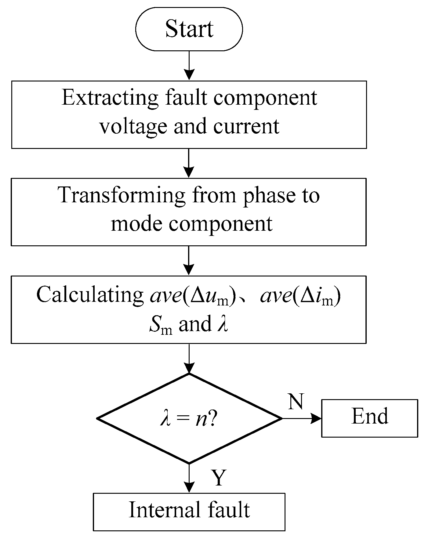
3. Identification Procedure of Busbar Protection

On the basis of the principle that is proposed in Section 2, for a busbar with n lines, the identification flowchart of the proposed protection is illustrated in Figure 5.

As shown in Figure 5, the procedure for identifying busbar fault is as follows:

• The protection adopts the startup elements, based on the change of the voltage and the current, and the protection starts when three successive samples satisfy Equations (16) or (17):

  $$\Delta i_p(k)=\left|i_p(k)-i_p(k-N)\right|\ge 0.2I_N$$

  (16)

  $$\Delta u_p(k)=\left|u_p(k)-u_p(k-N)\right|\ge 0.1U_N$$

  (17)

  where, p represents phase A, phase B, or phase C, i_p(k) and u_p(k) denote the kth sample of the fault current and voltage, respectively; Δi_p(k) and Δu_p(k) denote the kth sample of the fault component current and voltage, respectively; and I_N and U_N are the rated phase current and voltage, respectively. When one of all of the startup elements are connected to the bus operates, the relevant startup elements operate.
• Once a fault is detected, the busbar protection extracts the fault component voltage and fault component current for each line that is connected to the protected busbar at once.
• Then, the fault component voltage and fault component current of the three phases are transformed to the mode components, according to Equation (11), and the aerial mode y₁ will be used to calculate the average product.
• Further, using Equations (12)–(15), the ave(Δu_m), ave(Δi_m), S_m, and λ can be obtained.
• Finally, according to the value of λ, a fault inside or outside the busbar will be determined by the protection method.

4. Simulation and Analyses

4.1. Simulation Model

According to an effective 500 kV substation configuration and parameters, a busbar simulation model was built to testify to the effectiveness and practicability of the proposed busbar protection technique, as shown in Figure 6. Busbar I and busbar II were linked by three series circuit breakers and the model included four lines and two transformer branches. The researched objects were busbar I and busbar II. R₁, R₃, and R₅ formed a group to protect the busbar I. They utilized the currents of CT₁, CT₃, and CT₅, and the voltages of PT₁ (potential transformer), PT₃, and PT₅, respectively. While R₂, R₄, and R₆ extracted the currents of CT₂, CT₄, and CT₆ and the voltages of PT₂, PT₄, and PT₆, and then discriminated the running state of busbar II. The power lines adopted the frequency-dependent and transposition-uniform parameters. The length of each line is indicated in Figure 6. Defining the positive direction current for each line was the flow from the busbar to line. The sampling frequency that was used in the simulation was set at 4 kHz. Ten successive samples of the aerial components were used for the fault detection. The instant of the fault occurrence was generally at 0.5 ms without special explanation.

4.2. Adaptability Analysis of the Proposed Protection Principle

In Section 2, a busbar protection principle was proposed, and the theoretical analysis showed that the busbar protection criteria could discriminate between the internal faults and external faults for a single busbar configuration. However, whether the proposed protection principle was suitable for the complex busbar configurations or not, for example, that shown in Figure 6, needed further analysis. Note that the busbar I and busbar II were directly connected and very close because all of the middle circuit breakers were generally closed in the normal operation status.

4.2.1. Internal Fault

If a fault was to occur at f₁ on busbar I, the similar analysis as that of the single busbar configuration was as follows. Within the certain duration of the post-fault, the average products that were detected by R₁, R₃, and R₅ were all positive, which indicated a fault inside the busbar I. R₂, R₄, and R₆ should have all identified as the forward faults in theory, but it was unlikely that all of them could correctly identify the fault directions, because the busbar I and II were directly connected. Even so, the final identification result was still correct, because only if the discrimination results of the R₂, R₄, and R₆ were all backward faults, could the busbar II be considered as an internal fault.

4.2.2. External Fault

For a fault at f₂ on l₂, the theoretical analysis demonstrated that the average products that were detected by R₁ and R₂ were all negative during the specific time interval of the post-fault, so both the busbar I and busbar II were thought of as normal.

To summarize, the proposed busbar protection criterion should be fit for one and a half breakers of the busbar configuration. To verify the correctness of above analysis, the following simulations were executed.

4.3. Simulation of Typical Fault

4.3.1. Internal Fault

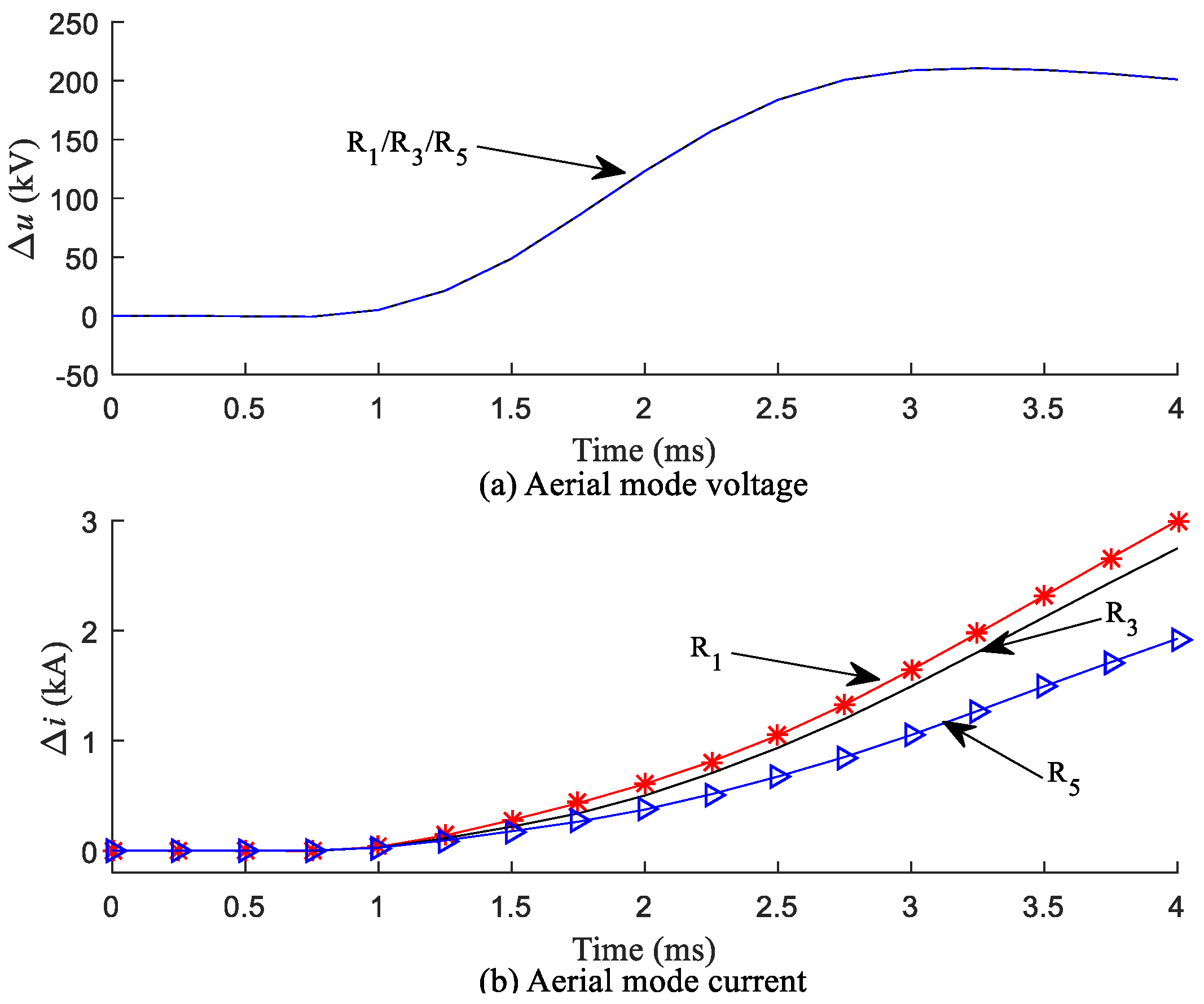
As shown in Figure 6, for a phase A grounding fault, at f₁ with a fault inception angle 30° and a fault resistance 25 Ω, Figure 7 and Figure 8 show the waveforms of the aerial mode voltage and aerial mode currents that were detected on each line of the busbars I and II, respectively. The corresponding average products are shown in

Table 1. Simulation results for a typical internal fault on busbar I.

Busbar	Protection Unit	S(kVA)	Fault Direction	λ	Identification Result
I	R1	1019.8	Backward	3	Internal Fault
	R3	892.7	Backward
	R5	650.6	Backward
II	R2	192.7	Backward	−1	External Fault
	R4	−106.5	Forward
	R6	−86.8	Forward

.

As shown in Figure 7 and Figure 8, within the specific time interval of the post-fault, the aerial mode voltages and currents for R₁, R₃, and R₅ were all positive. At the same time, the aerial mode voltages for R₂, R₄, and R₆ were also positive, however the aerial mode currents that were detected by R₂, R₄, and R₆ were not all positive. From Table 1, it can be seen that R₁, R₃, and R₅ had all identified the fault direction as backward, so a fault inside the busbar I could be determined. However, the detection units on busbar II verified that busbar II was normal. Therefore, the discrimination results were accurate.

4.3.2. External Fault

Assuming that a fault of the phase A grounding fault occurred at f₂ from busbar II at 20 km, the corresponding waveforms of the aerial mode components are depicted in Figure 9 and Figure 10, and the simulation data are listed in

Table 2. Simulation results for a typical external fault.

Busbar	Protection Unit	S (kVA)	Fault Direction	λ	Identification Result
I	R1	−360.7	Forward	1	External Fault
	R3	295.5	Backward
	R5	62.8	Backward
II	R2	−845.1	Forward	1	External Fault
	R4	422.3	Backward
	R6	419.9	Backward

.

From Figure 9 and Figure 10 and Table 2, it could be seen, within the short time of post-fault, that the sign of the aerial mode current for R₁ and R₂ was opposite to that of the aerial mode voltage, so R₁ and R₂ had identified the fault direction as forward. Even if the other protection units had verified that the fault directions were all backward, according to the criterion of the busbar protection, finally, an external fault was discriminated for both busbars I and II. Therefore, the discrimination results were all right.

4.4. Simulation for Fault with Diverse Initial Conditions

Generally, the performances of protection are affected by the fault initial conditions, such as the fault inception angle, fault resistance, and fault type [16]. The following simulations were carried out in order to evaluate the impact of the fault initial conditions on the method.

4.4.1. Different Fault Inception Angles

In general, for single-phase-grounding faults at f₁ on busbar I or at f₂ on l₂ with different fault inception angles,

Table 3. Simulation results of the different fault inception angles for the busbar I faults.

Unit	Ag 0°		Ag 15°		Bg 0°		Bg 200°		Cg 0°		Cg 310°
	S (kVA)	Result	S (kVA)	Result	S (kVA)	Result	S (kVA)	Result	S (kVA)	Result	S (kVA)	Result
R1	369.2	Internal	813.9	Internal	3632.2	Internal	19,666.7	Internal	7369.9	Internal	45,005.9	Internal
R3	316.8		704.0		3076.9		17,070.0		6286.4		39,859.1
R5	237.5		523.8		2220.8		12,244.6		4588.0		28,234.1
R2	66.8	External	148.5	External	721.8	External	3877.5	External	1422.7	External	8945.1	External
R4	−45.5		−95.5		−427.4		−2013.0		−868.7		−3974.4
R6	−22.1		−54.5		−306.3		−1886.1		−574.4		−4946.9

and

Table 4. Simulation results of the different fault inception angles for the external faults.

Unit	Ag 0°		Ag 30°		Bg 0°		Bg 60°		Cg 0°		Cg 200°
	S (kVA)	Result	S (kVA)	Result	S (kVA)	Result	S (kVA)	Result	S (kVA)	Result	S (kVA)	Result
R1	−83.3	External	−164.0	External	−833.2	External	−5163.7	External	−1653.4	External	−2456.1	External
R3	63.5		128.8		691.4		4268.7		1331.7		1995.9
R5	19.4		34.1		135.4		887.3		313.6		443.1
R2	−195.0	External	−386.6	External	−1994.1	External	−12,152.6	External	−3918.3	External	−5833.9	External
R4	91.1		184.3		987.7		6117.4		1902.3		2861.7
R6	103.4		200.9		998.7		6019.6		2005.2		2951.3

show the corresponding simulation data respectively.

The simulation data that are listed in Table 3 and Table 4 verified that the proposed technique could effectively discriminate between the internal faults and external faults with diverse fault inception angles. Moreover, the method could identify the faults with a zero inception angle in a high sensitivity.

4.4.2. Different Fault Resistances

Setting the phase A and phase B grounding faults at f₁ on busbar I with fault resistances of 50 Ω, 150 Ω, and 300 Ω, and the phase A and phase C grounding faults at f₂ on l₂ with fault resistances 0 Ω, 200 Ω, and 300 Ω, respectively, the simulation data are indicated in

Table 5. Simulation results of the different fault resistances for the busbar I faults and external faults.

Unit	ABg at f1						ACg at f2
	50 Ω		150 Ω		300 Ω		0 Ω		200 Ω		300 Ω
	S (kVA)	Result	S (kVA)	Result	S (kVA)	Result	S (kVA)	Result	S (kVA)	Result	S (kVA)	Result
R1	16,557.0	Internal	4037.7	Internal	1298.1	Internal	−3297.8	External	−314.0	External	−171.3	External
R3	14,646.4		3596.3		1159.9		2673.6		251.9		136.4
R5	10,350.9		2514.3		800.9		601.2		59.2		33.1
R2	3306.0	External	818.8	External	269.2	External	−7795.6	External	−734.7	External	−400.5	External
R4	−1461.5		−329.4		−98.6		3827.9		358.6		193.7
R6	−1847.4		−489.2		−169.9		3939.6		372.7		204.7

.

As shown in Table 4, as the fault resistance increased, the absolute values of the average products decreased to a certain extent, both for the internal faults and external faults. Nevertheless, the identification results were all correct.

4.4.3. Different Fault Types

For the different fault types at f₄ on busbar II, or at f₃ on l₃, the simulation data and identification results are shown in

Table 6. Simulation results of the different fault types for the busbar II faults.

Unit	Bg		Cg		ABg		ABCg		AB		AC
	S (kVA)	Result	S (kVA)	Result	S (kVA)	Result	S (kVA)	Result	S (kVA)	Result	S (kVA)	Result
R1	6167.3	External	1180.2	External	4004.9	External	7178.4	External	2325.5	External	1256.3	External
R3	1760.9		431.7		1173.4		2189.4		600.1		232.8
R5	−7935.3		−1598.3		−5176.3		−9334.9		−2925.3		−1505.9
R2	39,181.7	Internal	7819.1	Internal	25,531.1	Internal	46,328.2	Internal	14,427.4	Internal	7601.4	Internal
R4	28,278.0		5743.8		18,468.6		33,655.6		10,343.6		5340.0
R6	27,595.8		5381.1		17,929.2		32,573.2		10,193.4		5574.7

and

Table 7. Simulation results of the different fault types for the external faults.

Unit	Ag		Bg		ACg		BCg		AC		BC
	S (kVA)	Result	S (kVA)	Result	S (kVA)	Result	S (kVA)	Result	S (kVA)	Result	S (kVA)	Result
R1	318.9	External	1190.9	External	18,944.7	External	17,359.6	External	20,969.9	External	18,235.9	External
R3	−467.5		−1746.9		−28,122.1		−25,727.3		−31,130.8		−27,016.0
R5	147.3		549.7		9080.6		8278.6		10,057.5		8689.6
R2	213.6	External	786.2	External	12,540.1	External	11,431.9	External	13,886.4	External	11,997.6	External
R4	−284.4		−1074.5		−17,103.1		−15,728.8		−18,923.7		−16,533.4
R6	69.9		283.1		4484.1		4223.7		4953.6		4461.8

, respectively.

The simulation data shown in Table 6 and Table 7 indicates that the method could identify the faults with the different fault types exactly.

4.5. Other Influence Factors

4.5.1. Series Capacitor Compensation

In order to improve the EHV/UHV (Extra High Voltage/Ultra High Voltage) transmission capacity, series capacitors were generally installed in the long transmission lines. Therefore, it was essential to study the influence of the series capacitor compensation on the proposed technique. A series capacitor with a compensation coefficient of 40 percent was installed at the start of l_1, in Figure 7. The different faults were set at f₃, f₄, and f₅ and the simulation data is indicated in

Table 8. Simulation data for the series compensation.

Unit	f3		f4		f5
	S (kVA)	Result	S (kVA)	Result	S (kVA)	Result
R1	10,494.1	External	1254.9	External	−1205.6	External
R3	−15,591.1		305.3		786.2
R5	5044.0		−1571.6		423.6
R2	7007.6	External	7723.4	Internal	−439.6	External
R4	−9430.1		5484.6		284.8
R6	2379.6		5490.3		160.2

.

As shown in Table 8, whether the fault was on the compensated line or not, the proposed protection criterion could correctly discriminate all of these faults.

4.5.2. CT Saturation

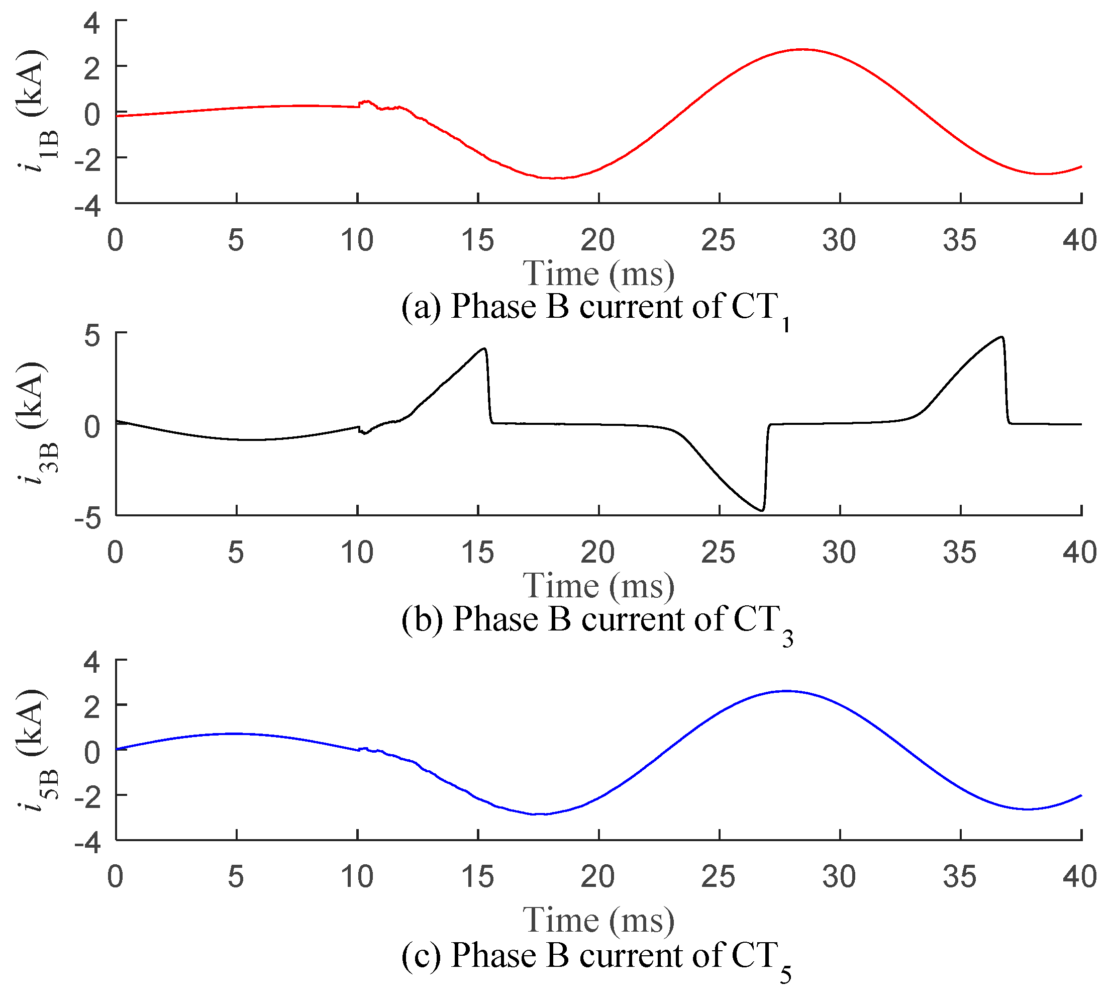
Generally speaking, the performance of the traditional busbar differential protection method is easily affected by CT saturation especially the serious CT saturation. Assuming a phase B grounding fault occurs at f₃ on l₃ with the phase B current of CT₃ seriously saturated to testify the effect of CT saturation on the proposed method. The waveforms of the phase B currents for CT₁, CT₃ and CT₅ are illustrated in Figure 11, and the differential currents of busbar I are shown in Figure 12. Figure 13 shows the waveforms of the calculated average products of busbar I, and

Table 9. Simulation results for a phase B fault on l₃.

Busbar	Protection Unit	S (kVA)	Fault Direction	λ	Identification Result
I	R1	248.5	Backward	1	External Fault
	R3	−371.6	Forward
	R5	125.4	Backward
II	R2	167.0	Backward	1	External Fault
	R4	−220.2	Forward
	R6	54.6	Backward

shows the corresponding simulation results. The instant of fault occurrence is 10 ms for Figure 11, Figure 12 and Figure 13.

From Figure 11, it can be seen that the phase B current of l₃ reached saturation after 5.16 ms of the post-fault. Meanwhile, Figure 12 shows the phase B differential current of busbar I, which increased from 0 to 5756 A. Consequently, the busbar differential protection of busbar I may maloperate. As shown in Figure 13 and

Table 10. Simulation results for a phase B fault on l₃.

Unit	Typical Internal Fault		Typical External Fault		Fault at f1
	S (kVA)	Result	S (kVA)	Result	S (kVA)	Result
R1	901.9	Internal	−16,383.0	External	1339.5	Internal
R3	797.9		13,572.1		2366.5
R5	577.9		4400.4		1689.4
R2	170.8	External	−37,689.2	External	1691.1	External
R4	−88.4		19,409.3		−783.8
R6	−82.8		18,264.1		−916.9

, it has been revealed that the CT saturation had no influence on the proposed busbar protection. This is because the identification criterion only used 2.25 ms of the data window of the post-fault, but at that time the CT saturation did not appear.

4.5.3. CVT Transfer Characteristic

The CVT (Capacitor Voltage Transformer) is currently widely used in the EHV/UHV power line, so the influence of the CVT transient transfer characteristic on the proposed algorithm could not be neglected. Setting the same fault conditions as the typical faults, in Section 4.3, and another phase B grounding fault at f₁ with the fault inception angle of 0°, and then, Table 10 shows the relevant simulation data.

As shown in Table 10, the proposed technique could identify these faults correctly, after taking the CVT transient transfer characteristic into account.

4.6. Operation Speed Analysis

The operation time of the busbar protection device basically included the filtering delay, phase-mode transformation, the calculation of the average product of aerial mode components, and the logical judgment, so it consumed little time. In view of the sampling frequency of 4 kHz, 10 consecutive samples, and the data window of 2.25 ms, the total time that used to detect a fault did not exceed 5 ms. Therefore, the novel busbar protection had a rapid operation speed.

5. Conclusions

This paper proposes a fast busbar protection method, based on the characteristic of the average product of the aerial mode components. Referring to an actual 500 kV substation, a simulation model was built and massive simulations were performed. From the theoretical analyses and simulation data, the following conclusions could be drawn:

• The busbar protection technique is applicable to both a single busbar configuration and one and a half breakers busbar configuration. Furthermore, the sampling frequency is set as 4 kHz, which is in accordance with the standard sampling frequency of the merging unit in the smart substation. Therefore, the method has a good adaptability.
• The performance of the proposed technique is hardly affected by the fault initial conditions, CT saturation, series compensation, and CVT transfer characteristic. Hence, the method has high reliability and sensitivity.
• The proposed technique has a rapid operation speed, and the operation time is usually less than 5 ms.

References

- Panfeng, W.; Xiaolong, Z.; Huihong, Y. A scheme of busbar protection in digital substation. Power Syst. Prot. Control 2009, 37, 48–51. [Google Scholar]
- Fengmei, C.; Xiaozhou, S.; Yingli, Q. Research on distributed busbar protection based on digital substation process level. Electr. Power Syst. 2008, 32, 69–72. [Google Scholar]
- Guibin, Z.; Xiaogang, W.; Houlei, G.; Baoji, Y. Distributed busbar protection of digital substation. Electr. Power Autom. Equip. 2010, 30, 94–97. [Google Scholar]
- Femandez, C. An Impedance-based CT saturation detection algorithm for bus-bar differential protection. IEEE Trans. Power Deliv. 2001, 16, 468–472. [Google Scholar] [CrossRef]
- Kang, Y.C.; Kang, S.H.; Crossley, P.A. Design, evaluation and implementation of a busbar differential protection relay immune to the effects of current transformer saturation. IEE Proc. Gener. Transm. Distrib. 2004, 151, 305–312. [Google Scholar] [CrossRef]
- Yong-Cheol, K.; Ui-Jai, L.; Sang-Hee, K.; Crossley, P. A busbar differential protection relay suitable for use with measurement type current transformers. IEEE Trans. Power Deliv. 2005, 20, 1291–1298. [Google Scholar] [CrossRef]
- Kang, Y.C.; Yun, J.S.; Lee, B.E. Busbar differential protection in conjunction with a current transformer compensating algorithm. IET Gener. Transm. Distrib. 2008, 2, 100–109. [Google Scholar] [CrossRef]
- Watanabe, H.; Shuto, I.; Igarashi, K. An enhanced decentralized numerical busbar protection relay utilizing instantaneous current values from high speed sampling. In Proceedings of the 2001 7th International Conference Developments in Power System Protection, Amsterdam, The Netherlands, 9–12 April 2001. [Google Scholar]
- Ge, Y.Z.; Dong, X.L.; Dong, X.Z. A new bus-bar protection based on current travelling wave and wavelet transform (1)-basic principle and criterion. Trans. China Electrotech. 2003, 18, 95–99. [Google Scholar]
- Li, W.; Wang, Q.; Du, Y.H. Extraction of transient character based on the mathematical morphology for distributed bus protection. Power Syst. Prot. Control 2009, 37, 11–15. [Google Scholar]
- Li, H.F.; Wang, G.; Li, X.H. A novel busbar protection based on transient current spectrum energy. Autom. Electr. Power Syst. 2005, 29, 51–54. [Google Scholar]
- Zou, G.B.; Gao, H.L. A travelling-wave-based amplitude integral busbar protection technique. IEEE Trans. Power Deliv. 2012, 27, 602–609. [Google Scholar] [CrossRef]
- Song, S.L.; Zou, G.B. A Novel Busbar Protection Method Based on Polarity Comparison of Superimposed Current. IEEE Trans. Power Deliv. 2015, 30, 1914–1922. [Google Scholar] [CrossRef]
- Hashemi, S.M.; Hagh, M.T.; Seyedi, H. Transmission-line protection: A directional comparison scheme using the average of superimposed components. IEEE Trans. Power Deliv. 2013, 28, 955–964. [Google Scholar] [CrossRef]
- Song, S.L.; Zou, G.B.; Gao, H.L. A fast busbar protection based on the average of superimposed components. In Proceedings of the International Conference on Electrical and Electronic Engineering (EEE), Hong Kong, China, 10–12 April 2014. [Google Scholar]
- Zou, G.B.; Gao, H.L. Fast pilot protection method based on waveform integral of traveling wave. Int. J. Electr. Power Energy. Syst. 2013, 50, 1–8. [Google Scholar] [CrossRef]
Figure 1.
Fault circuit of a simple busbar structure.
Figure 2.
The (a) fault superimposed network when a fault at f1 on busbar B occurs. The (b) fault superimposed network when a fault at f2 on l1 occurs.
Figure 3.
Δu1, Δi1, and S1 detected by R1 for an internal busbar fault.
Figure 4.
Δu1, Δi1, and S1 detected by R1 for a fault on l1.
Figure 5.
Identification flowchart of the busbar fault.