Task Space Trajectory Planning for Robot Manipulators to Follow 3-D Curved Contours


1
Korea Institute of Robotics & Technology Convergence, Pohang 37553, Korea
2
Department of Mechanical Engineering, Korea National University of Transportation, Chungju 27469, Korea
*
Authors to whom correspondence should be addressed.
Electronics 2020, 9(9), 1424; https://doi.org/10.3390/electronics9091424
Submission received: 24 July 2020
/
Revised: 30 August 2020
/
Accepted: 31 August 2020
/
Published: 2 September 2020
(This article belongs to the Special Issue Modeling, Control, and Applications of Field Robotics)
Abstract
:The demand for robots has increased in the industrial field, where robots are utilized in tasks that require them to move through complex paths. In the motion planning of a manipulator, path planning is carried out to determine a series of the positions of robot end effectors without collision. Therefore, it is necessary to carry out trajectory planning to determine position, velocity, and acceleration over time and to control an actual industrial manipulator. Although several methods have already been introduced for point-to-point trajectory planning, a trajectory plan which moves through multiple knots is required to allow robots to adapt to more complicated tasks. In this study, a trajectory planning based on the Catmull–Rom spline is proposed to allow a robot to move via several points in a task space. A method is presented to assign intermediate velocities and time to satisfy the velocity conditions of initial and final knots. To optimize the motion of the robot, a time-scaling method is presented to minimize the margin between the physical maximum values of velocity and acceleration in real robots and the planned trajectory, respectively. A simulation is then performed to verify that the proposed method can plan the trajectory for moving multiple knots without stopping, and also to check the effects of control parameters. The results obtained show that the proposed methods are applicable to trajectory planning and require less computation compared with the cubic spline method. Furthermore, the robot follows the planned trajectory, and its motion does not exceed the maximum values of velocity and acceleration. An experiment is also executed to prove that the proposed method can be applied to real robotic tasks to dispense glue onto the sole in the shoe manufacturing process. The results from this experiment show that the robot can follow the 3-D curved contour in uniform speed using the proposed method.
1. Introduction
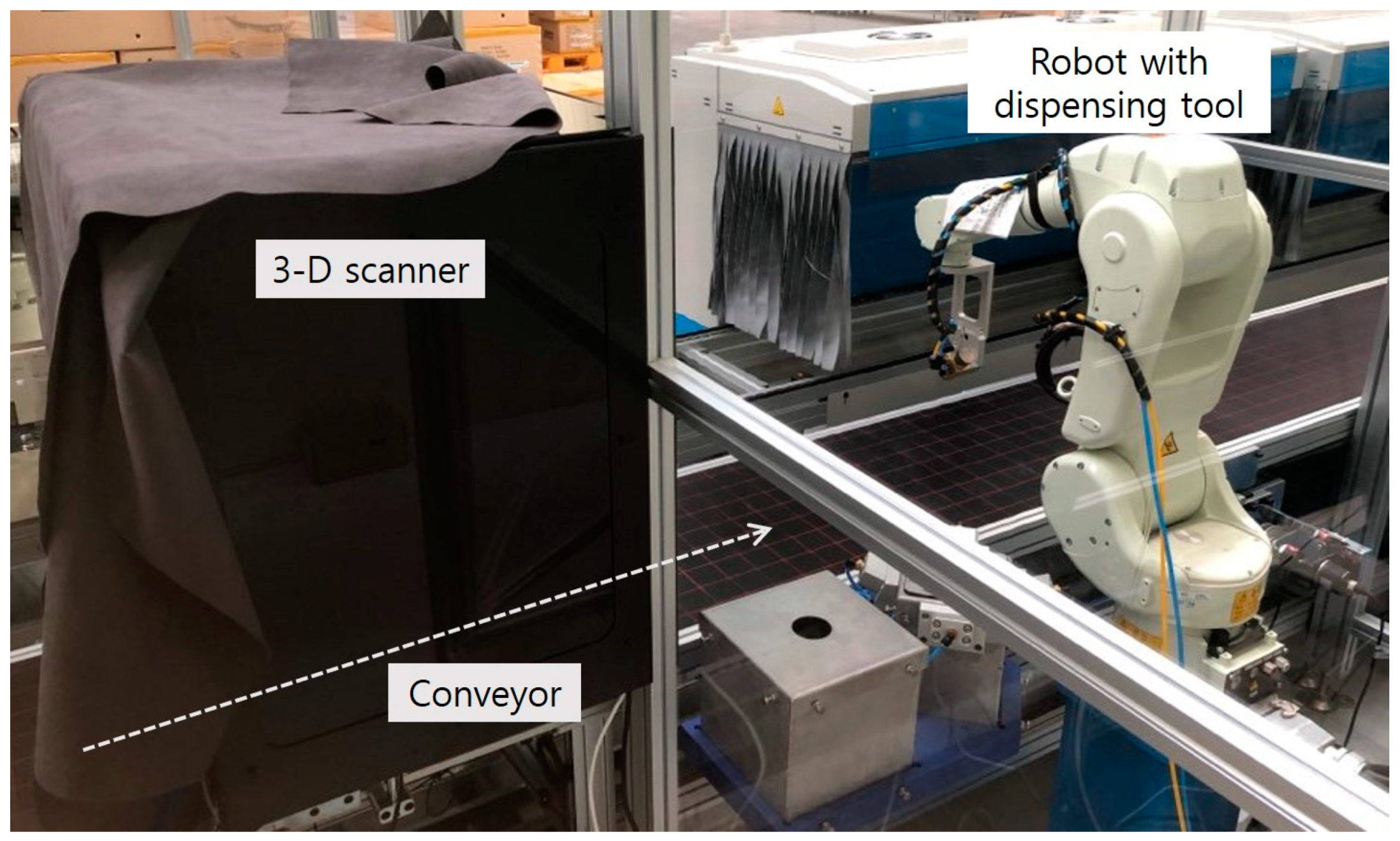
Owing to growing interest in industrial robots, various robots have been utilized in manufacturing sites. Previously, in the teaching process, skilled operators manually moved a robot and recorded its position in the robot controller. The recorded position was then replayed by performing a point-to-point or continuous-path motion in a real robot [1,2,3]. Using this teaching process, the robot can execute pick and place, loading and unloading, and assembly tasks in the manufacturing site. However, for the same robot to adapt to more complex and flexible tasks such as painting, polishing, welding, etc., the complicated and optimal paths or trajectory planning methods are required [4,5,6,7,8,9]. One of the core processes in a shoe manufacturing factory [10] is attaching a sole to the upper part of a shoe, after applying adhesive to the upper contour of the sole. If a robot is adapted to this gluing task, its Tool Center Point (TCP) should follow the 3-D contour path of the sole with a uniform dispensation of the glue. For the robot to move through this contour, a trajectory should be planned a priori. This trajectory is planned by connecting intermediate points on the contour obtained from the CAD data of the sole or from the point cloud scanned in the 3-D scanner while the target object is being moved by a conveyor, as shown in Figure 1.
If the robot moves several consecutive points without stopping at each point, a smooth spline path is required to avoid discontinuity of velocity. The points through which the robot passes are called knots or knot points. This spline method has been widely applied to create paths for many systems such as mobile robots [11], vehicles [12], unmanned aerial vehicles (UAVs) [13], and manipulators [14,15]. Actual examples of robotic tasks include welding, dispensing glue, and painting, where a manipulator must move continuously through multiple defined knots in a manufacturing site.
In the motion planning of the robot, path planning is used to find a series of the positions of robot end effectors without collision. However, in trajectory planning, it is necessary to move the real manipulator to determine the position, velocity, and acceleration of the robot over time. Sampling-based motion planning [16] is widely used in path planning to find a collision-free path. However, it cannot be used to derive closed-form solutions to plan this trajectory. To apply to industrial robots, closed-form solutions are required to assign a position, velocity, and acceleration to them at each sampling time. Consequently, previous studies used other methods such as B-spline, cubic spline, trigonometric spline, and Bezier spline to plan a trajectory for multi-points [17,18,19,20,21,22,23,24,25,26]. The spline trajectory planning method can be divided into trajectory planning in the joint space and trajectory planning in the task space (Cartesian coordinate space). In the joint space, the cubic spline method is primarily used to generate the trajectory of each joint such that the change in angle of each joint is connected without stopping during motion. The joint vector at each knot should be calculated using inverse kinematics before applying the trajectory planning method. In the concept of the trajectory planning in the task space, the time series of position in the task space are derived at every sampling time. Then the joint vectors at each sampling time are calculated with inverse kinematics and the robot controller moves joint angles. Basically, the operators intuitively assign and record each knot of the manipulator in the real manufacturing site. Therefore, it is necessary to propose a new method to plan spline trajectory in the task space.
In the task space, the Catmull–Rom spline can be used to plan the spline path [27] because it is simple and requires little computation. The Catmull–Rom spline is primarily used in computer graphics applications to draw paths that connect multiple points smoothly [28], in order to satisfy the continuity of velocity at each point [29]. At these points, Catmull–Rom can be applied to plan the trajectory of the robot manipulator. However, it is necessary to first derive the velocity and acceleration functions for the trajectory planning of the robot. A method is required to assign initial and final velocities while a systematic consideration is necessary to plan the trajectory for complicated industrial applications such as following a closed-loop contour at uniform speed. To apply this to the robot, it is necessary to maximize productivity by minimizing its cycle time [30]. Previous studies considered this problem and proposed a method for an optimal trajectory using jerk bounding [31,32] or by considering velocity and acceleration [33]. However, determining the jerk limit of a robot is difficult and counterintuitive [34]. Therefore, it is necessary to optimize the velocity and acceleration of the robot considering limit conditions such as maximum speed and acceleration.
In this study, a simple novel method is proposed to generate a spline trajectory in a task space to allow the robot to move through multiple knots. To help the basic Catmull–Rom spline adapt to the robot trajectory planning problem, the authors propose an iterative segmentation method for multiple knots and present a method that determines control points outside the trajectory, such that the initial and final velocities of the motion are zero. To minimize the operating time of the robot and stay within the physical limit value, an optimization method that considers the physical maximum velocity and acceleration of the robot is presented. The systematic planning process is presented for applications in complicated industrial tasks, to enable the robot to follow the 3-D contour at uniform speed. The proposed methods are evaluated via simulation in various cases and to compare computational load with the cubic spline method. They are also implemented with an experiment that involves dispensing adhesive uniformly to the upper contour of the sole of a shoe at a shoe manufacturing factory. The results show that the proposed trajectory planning in the task space can be applied to the robotic task in actual manufacturing processes.
Section 2 introduces related studies and a basic Catmull–Rom spline in detail. In Section 3, the method for creating the task space trajectory based on the Catmull–Rom spline is explained with the simulation. An experiment to test the proposed method on real industrial robotic tasks are described in Section 4. Finally, Section 5 contains the discussion and conclusion of this study.
2. Trajectory Planning via Spline Method
2.1. Related Works
Several studies have focused on trajectory planning using smooth functions to connect multiple knots [17,18,19,20,21,22,23,24,25,26]. There are two types of trajectory planning, namely, interpolation and approximation. When a series of knots is given, interpolation is the method used to pass a robot completely through the actual knots. The approximation method involves determining the smooth function from the knots but does not aid the passage through the actual knots [17,18].
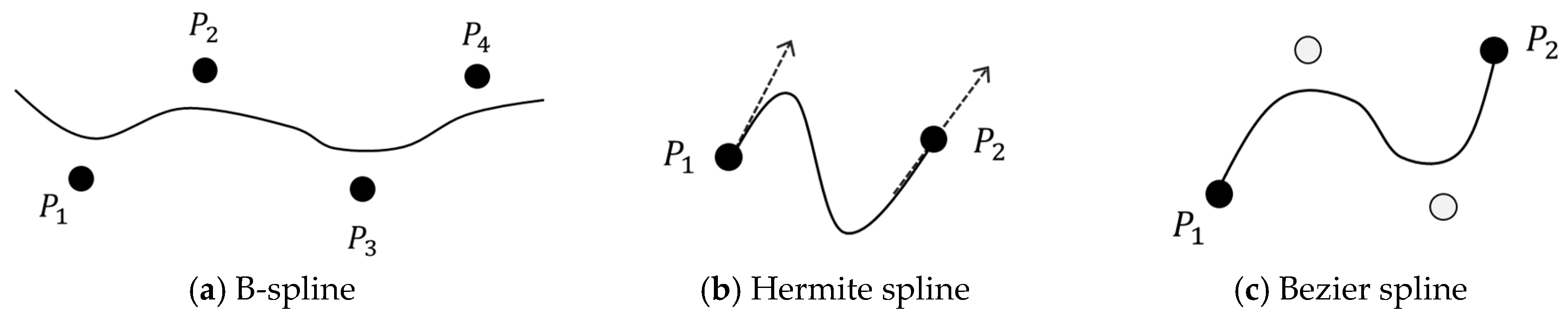
A commonly used approximation method in the robotics application is the B-spline [19,20,21]. B-splines blend the positions of control points without passing through any of them, as shown in Figure 2a. It is used in the computer graphics area, which has a curve that consists of the linear combination of B-spline basic functions, with control points determining the shape of the curve. B-spline is widely used because it can be easily and quickly modified when a local modification is necessary. Koch and Wang [19] applied B-spline to planning the joint trajectory of manipulators. Biagiotti and Melchiorri proposed a simple method to formulate B-spline-based trajectories with simplicity and low computational complexity [20]. Haron et al. proposed a new parameterization method that can handle collinear and two adjacent data points, including long distances between two consecutive data points [21]. Although previous research on B-spline has been published, it is basically just an approximation method and cannot be applied to a task that requires the curve to pass through waypoints.
The Hermite formulation is one of the popularly recognized functions used for interpolations. To obtain a Hermite spline as shown in Figure 2b, an operator must collinearly arrange consecutive tangents to satisfy velocity continuity [17]. Applying this method to robotic tasks is tedious because it requires all tangential vectors for all knots to be assigned. Previous research reported that the Bezier spline is well suited for robotic motion planning [16,22]. The smooth curve is constructed by adding two control points in the cubic Bezier curve case, as shown in Figure 2c. The 3rd order Bezier curve has continuity in velocity and acceleration by adding two control points. If more than two control points are placed inside the path, the order of the equation increases and the curve becomes smoother than it was before [22]. However, it is difficult to add and determine the positions of control points when multiple knots are given because control points can be arbitrarily placed. In addition, the path cannot pass the control points exactly.
The cubic spline in references [23,24] provides a simple method to generate a smooth robot trajectory. Here, the piecewise-cubic trajectory, which passes through the waypoints and satisfies velocity continuity can be determined. The cubic spline has been used for joint [3] and task space trajectory splines [23]. Kolter and Ng proposed a method for task space trajectory planning using cubic spline optimization. However, one setback of the cubic spline is its computational limitation because it needs additional processes to compute intermediate velocities in order to find the function of the curve [2,23]. A cubic spline interpolation with three control points was then proposed in reference [24] to overcome the Catmull–Rom spline using four points. They applied the proposed method to limited cases and compared it with the method using the Catmull–Rom. They mentioned that it could exhibit undesirable behaviors such as large overshoot compared with the case using the Catmull–Rom. Other methods such as trigonometric function and polar piecewise were also proposed [25,26]. However, they are not widely used because they can only be applied to specific types of robots or have limitations to their smoothness.
This study aimed to plan the trajectory for a robot to follow the 3-D contour of a sole at a shoe manufacturing factory. When intermediate points on the edge of the sole are given, it is necessary to adopt the interpolation method to connect all given waypoints on the Cartesian space. If the 3rd order Bezier spline is used for this case, two control points should be placed between every two neighboring knots. It is tedious to plan the trajectory and the trajectory can be changed depending on the positions of the control points. There was no interest in approximation in this study. Consequently, the planned trajectory meets certain requirements [24]. The first requirement was that it should be at least continuous. The continuity of the position and velocity at each point had to be satisfied. The second requirement was that it had to be an interpolating spline to pass through all given waypoints. The most used interpolating splines that satisfy these two requirements are Catmull–Rom splines. The Catmull–Rom satisfies the continuity of velocity at each point [27,28,29] and can be used intuitively in the task space. The Catmull–Rom spline makes use of positions on the knots alone without any other information such as tangent for velocity in Hermite.
To apply the Catmull–Rom spline to the trajectory planning of a robot, it is crucial to select two control points before and after the path connecting the two given points. In this study, iterative segmentation was proposed to interpolate consecutive points by assigning control points from neighboring knots without any arbitrary determination of control points. Additionally, the method used to select the first and final control points was addressed to satisfy the condition that requires both the initial and final velocities of the trajectory to be zero.
2.2. Catmull–Rom Spline
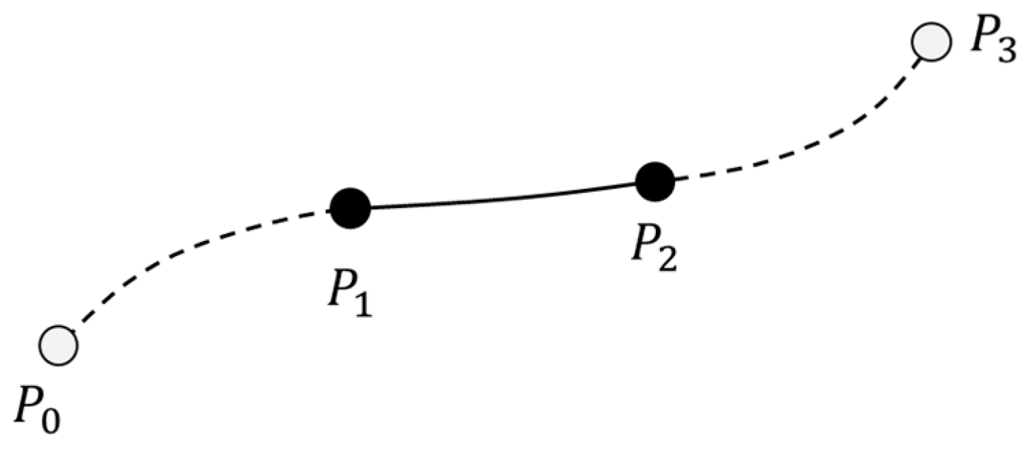
The Catmull–Rom spline method is used to interpolate the path between two given points ( and ). In the Catmull–Rom spline method, two virtual control points ( and ) are assigned before and after the path connecting the two given points ( and ), as shown in Figure 3. Because the curvature of the path changes with the two control points outside the path, the method used to set these control points must be considered.
When the position of the robot is at time , it is referred to as , and the constraint conditions for this position and its velocity are expressed in Equations (1) and (2), respectively. When is 0.5 in the Catmull–Rom spline case in reference [26], the tangents of and are determined from the difference between the neighboring two points as defined in Equation (2).
To create an actual trajectory, it is necessary to determine the time at each midpoint (knot). In reference [28], the parameterization of the Catmull–Rom curve is defined using the parametric value in Equation (3). In this study, time was replaced with , and the time at each point could be determined by in Equation (4). As a parameter, was used for determining the time at each point using a value between zero and one. In the case of a zero value, all sections between two neighboring points are referred to as uniform splines of the same time. When is set to one, they are referred to as chordal splines proportional to the relative distance. However, in a uniform spline case, self-intervention can be generated. This is not appropriate because a large acceleration may be generated by a small radius of curvature owing to the rapid change of path when the robot follows this trajectory. In a chordal spline case, a moving distance becomes long in a relatively gentle path, which is disadvantageous. Another case is the centripetal spline case, which has a value of 0.5.
When the time at each point is determined using Equation (4), the position of the trajectory with respect to time is expressed in Equation (5). For simplicity, the equations are represented by parameters of and . is a function of time determined by position, and , and time, and , of the neighboring two knots. is a function of time determined by and , and and .
where,
To derive this trajectory, velocity and acceleration should be solved. The velocity function in Equation (6) is derived by differentiating the position function defined in Equation (5) with respect to time, and the acceleration function in Equation (7) can be obtained by differentiating Equation (6) with respect to time.
where,
where,
3. Trajectory Planning for Multiple Knots
3.1. Iterative Segmentation for Multiple Knots
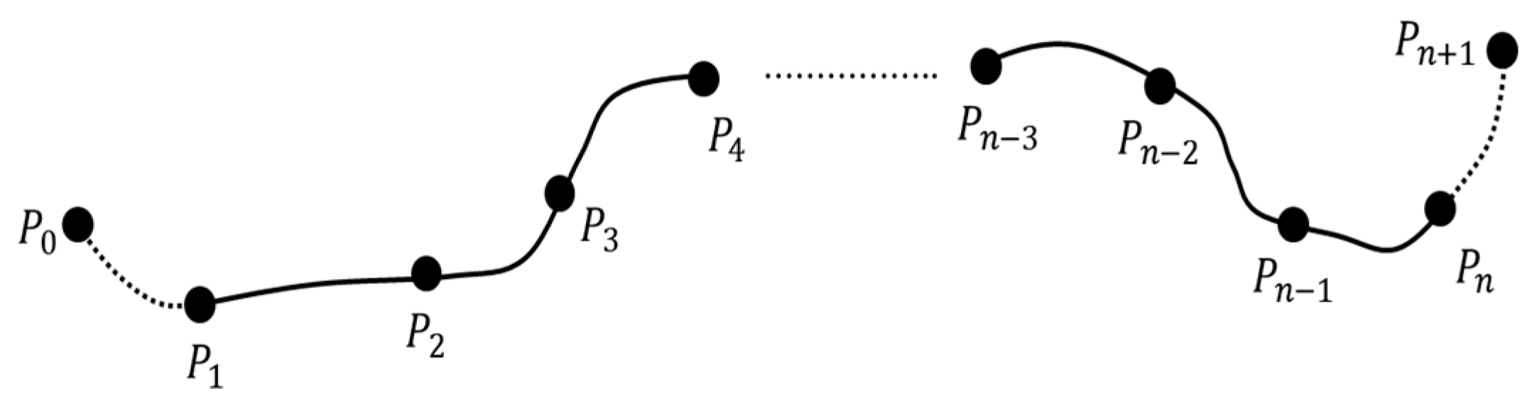
The Catmull–Rom spline is basically utilized to find paths in order to connect two points. Therefore, the Catmull–Rom spline method should be sequentially applied by connecting two consecutive neighboring points to generate a trajectory via multiple knots. Figure 4 shows an example of n knots starting at up to .
To connect and in the first segment, two control points are required. One control point can be designated as the next knot . For the other control point, a virtual control point can be selected using the constraint that maintains the velocity at at zero because is the starting position in the overall path. From Equation (2), the velocity at is zero when is equal to , as expressed in Equation (8).
To derive the path in the subsequent segment, two control points are placed using the points that immediately precede and follow them. When the last segment connects to , similar to the first segment, the virtual control point can be replaced with , such that the velocity at becomes zero in Equation (9). Therefore, the first control point and last control point of the entire trajectory can be determined. Equations (5)–(7) can be applied repeatedly to obtain the position, velocity, and acceleration of the entire trajectory.
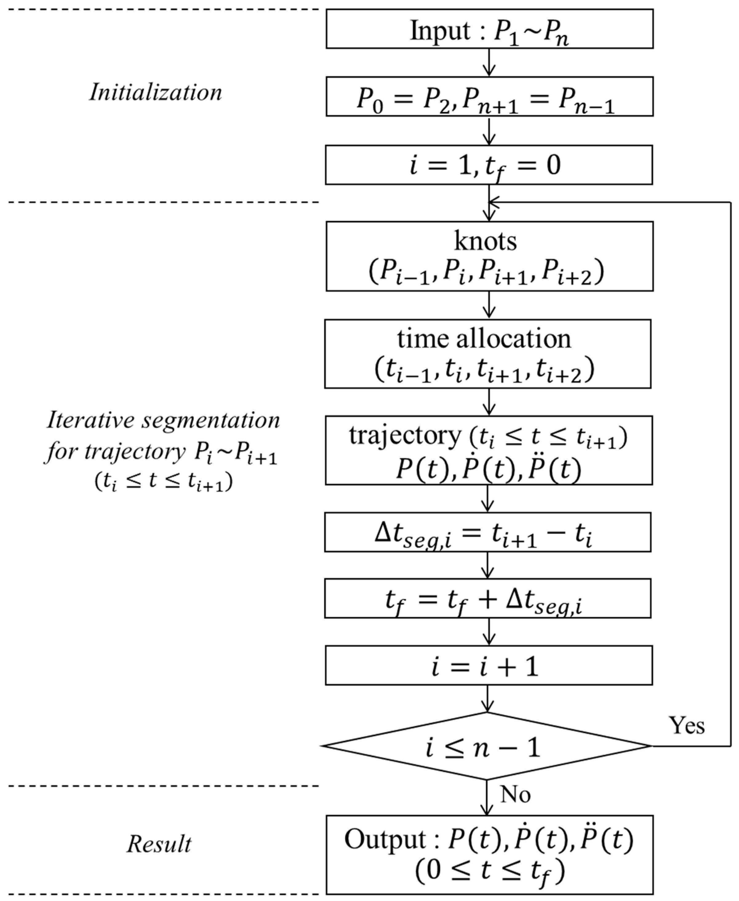
The process to plan trajectory from to is represented as a flowchart in Figure 5. Two virtual control points, and , are assigned using (8) and (9) when the n multiple knots are given. Every four knots are selected as a segment from to , and trajectory from to are iteratively calculated using Equations (4)–(7). Then position, velocity, and acceleration for the entire path can be derived as a result and final motion time can be found as . Simulation to evaluate the proposed method is performed with MATLAB in the computer operated by Windows operating system. The source code for the algorithm is implemented as a script language in MATLAB without using a toolbox.
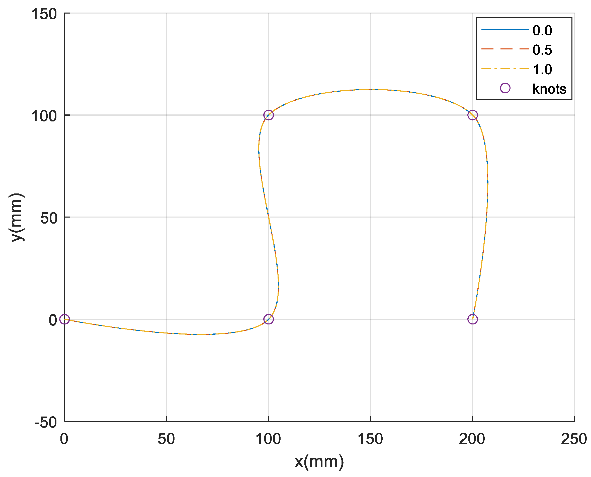
The simulations used to move multiple knots in the task space are executed using data in Table 1. The first simulation is implemented to show trajectory planning when all segments have an equal distance with knots in the task #1. In the second simulation, each segment has a different distance as knots in the task #2.
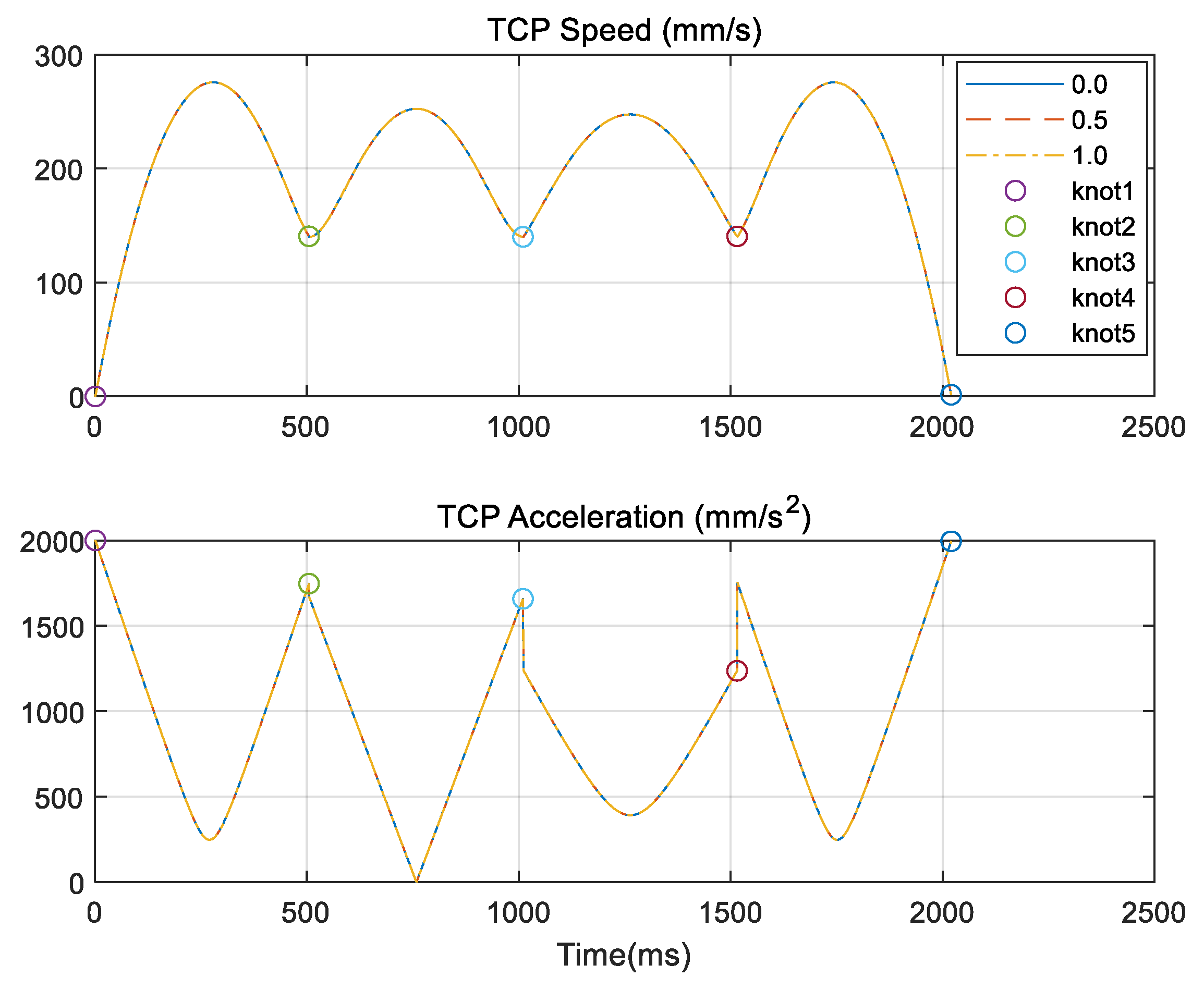
The target path in the task #1 consists of five points, and the distance between two points in each segment is 100 mm. The result of the planned path using the proposed method is shown in Figure 6. The given knots are represented as a circle at each point, and each line corresponds to the case when in Equation (3) is changed from 0 to 1. The velocity and acceleration of the TCP of the robot are shown in Figure 7. The results show that the three trajectories are exactly the same even when a different is applied. The velocity at the initial or final point is zero, and the trajectory exhibits continuity in velocity at each point. This shows that the trajectory remains consistent regardless of the value of , provided all segments are uniform in length.
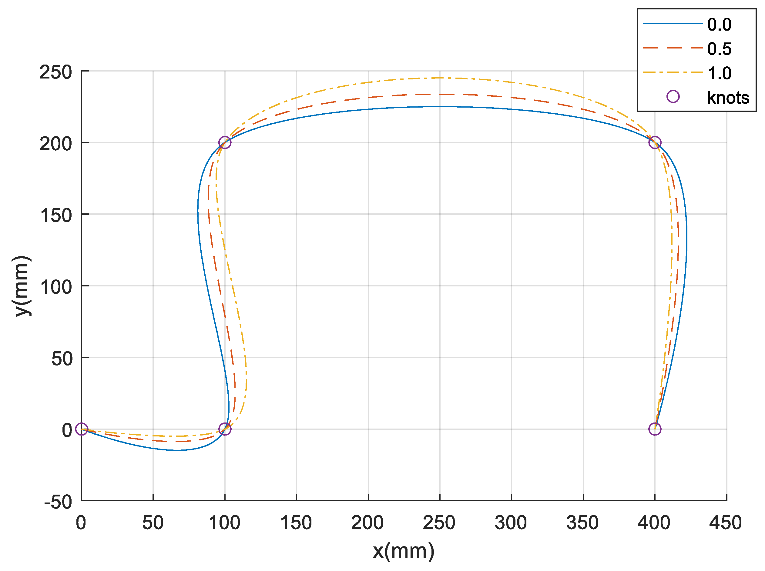
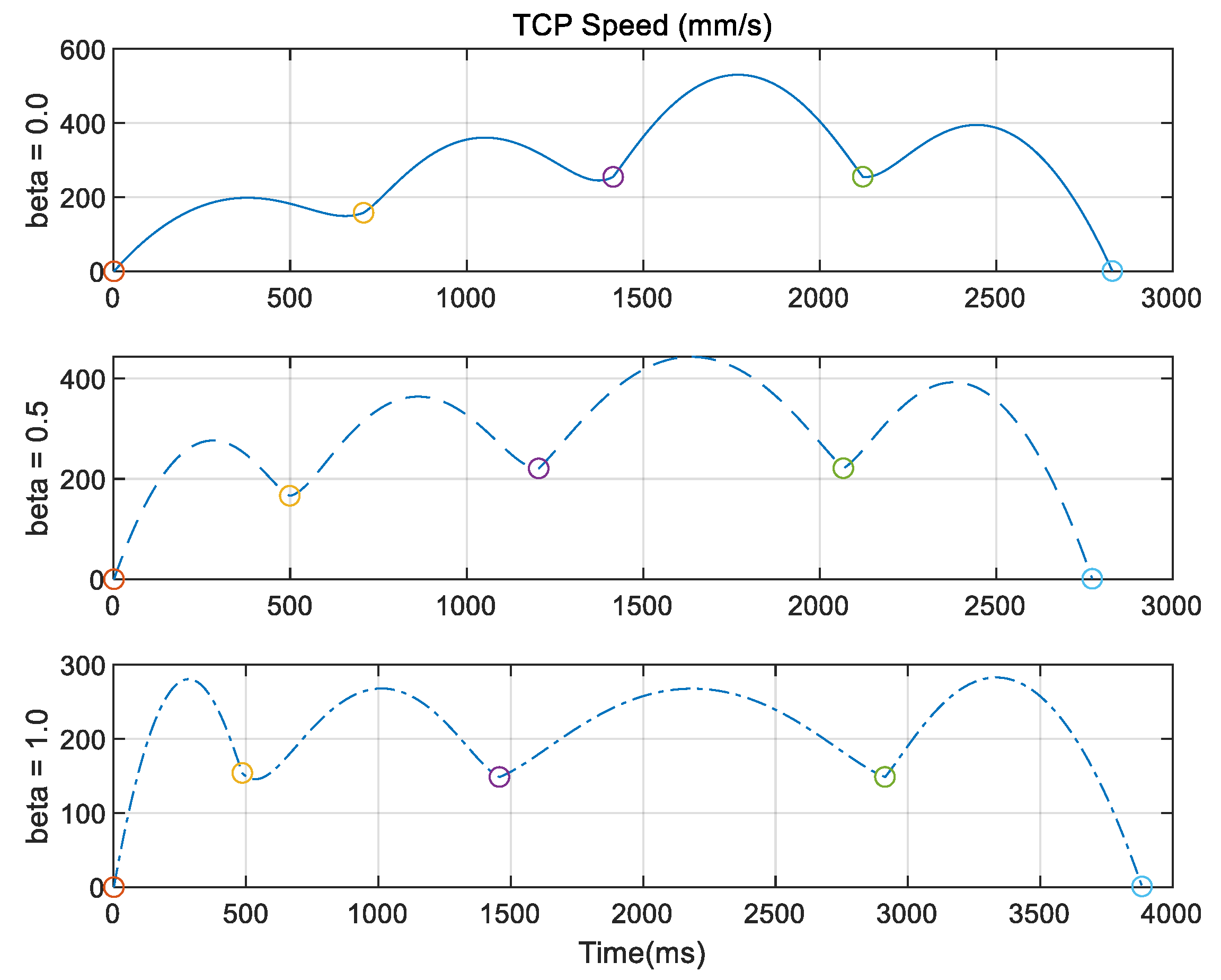
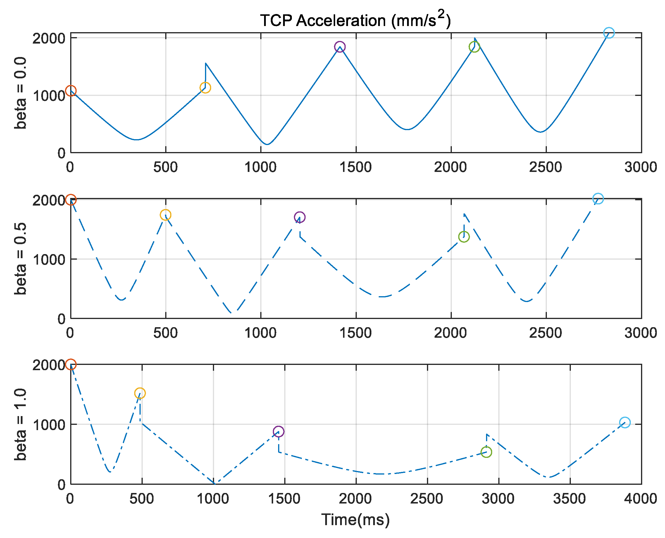
In the second simulation with the task #2, each segment has its own distance, from 100 mm to 300 mm. The result of the planned path is shown in Figure 8 and its velocity and acceleration profiles are represented in Figure 9 and Figure 10, respectively. As shown in these figures, the path and trajectory change according to the value of . As shown in the third segment with the longest distance between points 3 and 4, a long motion time is required and this motion follows the long path in the chordal case (). This occurs because the time in each segment is proportional to the relative distance between two points. However, the deviation in the velocity at each segment is relatively small when is one. Therefore, if the robot is required to move at a relatively uniform speed to execute the spline motion, can be chosen as one.
3.2. Comparison with Cubic Spline
The proposed method based on the Catmull–Rom spline is compared with the previous spline method used in the interpolation. The representative method is the planning using a cubic spline curve. It has a piecewise-cubic trajectory, which passes through the multiple waypoints and satisfies velocity continuity at each waypoint. The simulation is implemented using knots in the task #1 and the task #2 to show computational efficiency and shape of the curve.
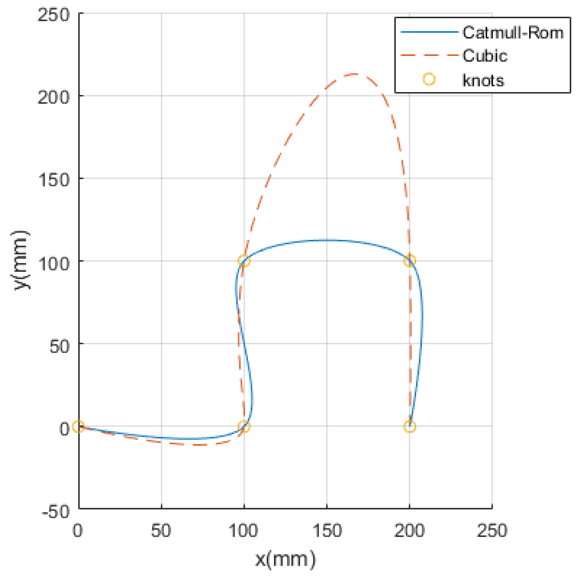
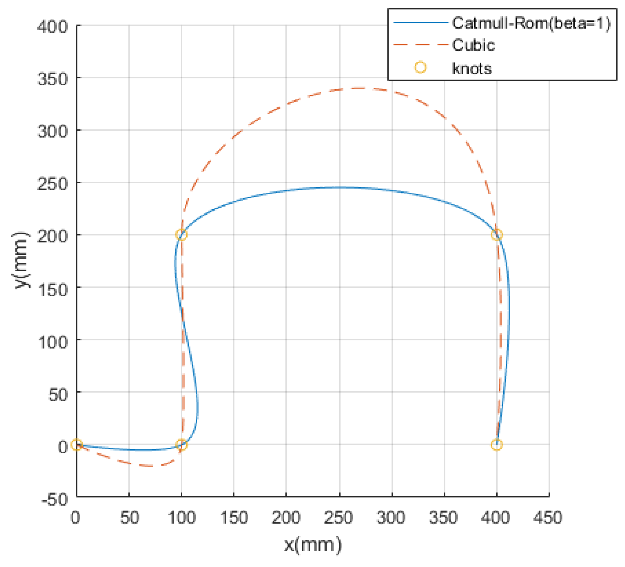
In Figure 11 and Figure 12, the difference between the two results can be shown. The paths are compared in Figure 11 when knots in the task #1 are used for planning. A large overshoot exists between the third and fourth waypoints when the cubic spline is applied. Figure 12 shows the paths from knots in the task #2 and a large overshoot can be shown in the same segment. It means that the curve using cubic spline can exert large overshoot as mentioned in reference [24].
The computation time is measured while these simulations are executed to compare computational efficiency for two methods. This simulation is performed with MATLAB in the computer operated by Windows 10. It has an Intel Core i7 4 GHz CPU with 32 GB RAM. The 20 simulations are performed, and the average time and standard deviation are listed in Table 2. The results show that it takes less time in about 5.7~5.8 ms when the Catmull–Rom is used compared with cubic spline. Therefore, it can be concluded that the proposed method requires less computation.
3.3. Optimization of Velocity and Acceleration
Because the trajectory generated by the iterative segmentation procedure is determined by the time passed by each point in Equation (4), the physical maximum velocity and acceleration of the actual robot are not considered in the magnitudes of the velocity and acceleration. To minimize the operating time of the robot and maintain its physical limit value, it is important that velocity and acceleration would cause the trajectory to move lower and closer to the maximum velocity and acceleration to which the robot can move.
The points where the velocity and acceleration of the robot are maximum in the trajectory are those points where the derivatives of its position and velocity are zero. The time corresponding to the trajectory of the actual robot movement in one segment is between and . The maximum velocity and acceleration in each segment can be estimated from Equations (6) and (7). When these values are determined in the entire segments, the maximum velocity and maximum acceleration can be predicted in the entire trajectory.
To optimize the velocity and acceleration of motion and enable the robot to follow the planned trajectory, the maximum velocity and the maximum acceleration in the task space of the real robot should be determined. If the initial and final velocities in the trajectory are zero, the maximum velocity and maximum acceleration of the robot can be changed according to the ratio of the motion time. The parameters and representing this ratio can be calculated using Equation (10) because the velocity is linear with time and acceleration is proportional to the square of time. By determining the maximum ratio value in Equation (11) and multiplying it by the motion time , the optimized motion time can be obtained, as expressed by Equation (12). Hence, by redistributing the motion time according to this ratio, the actual velocity and acceleration of the robot can be approximated to the physical maximum value, and the motion of the robot can be optimized.
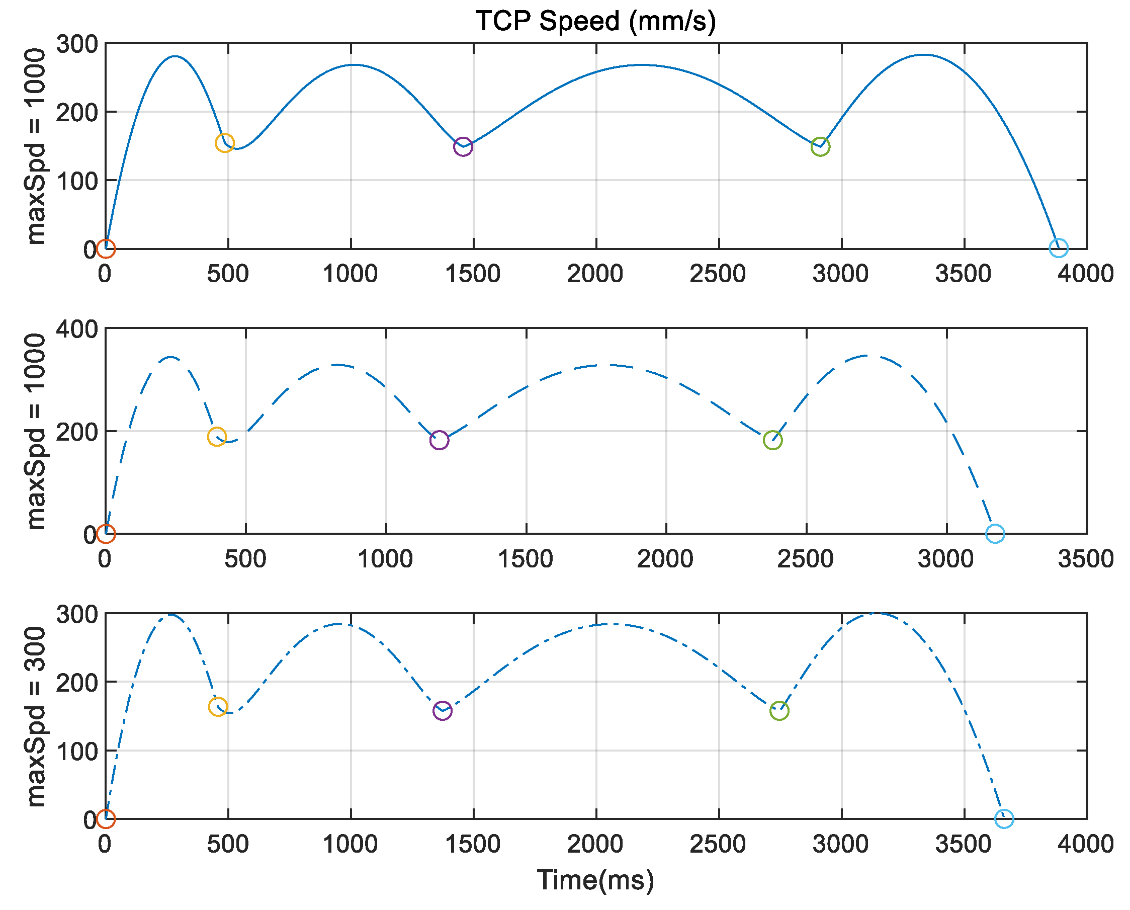
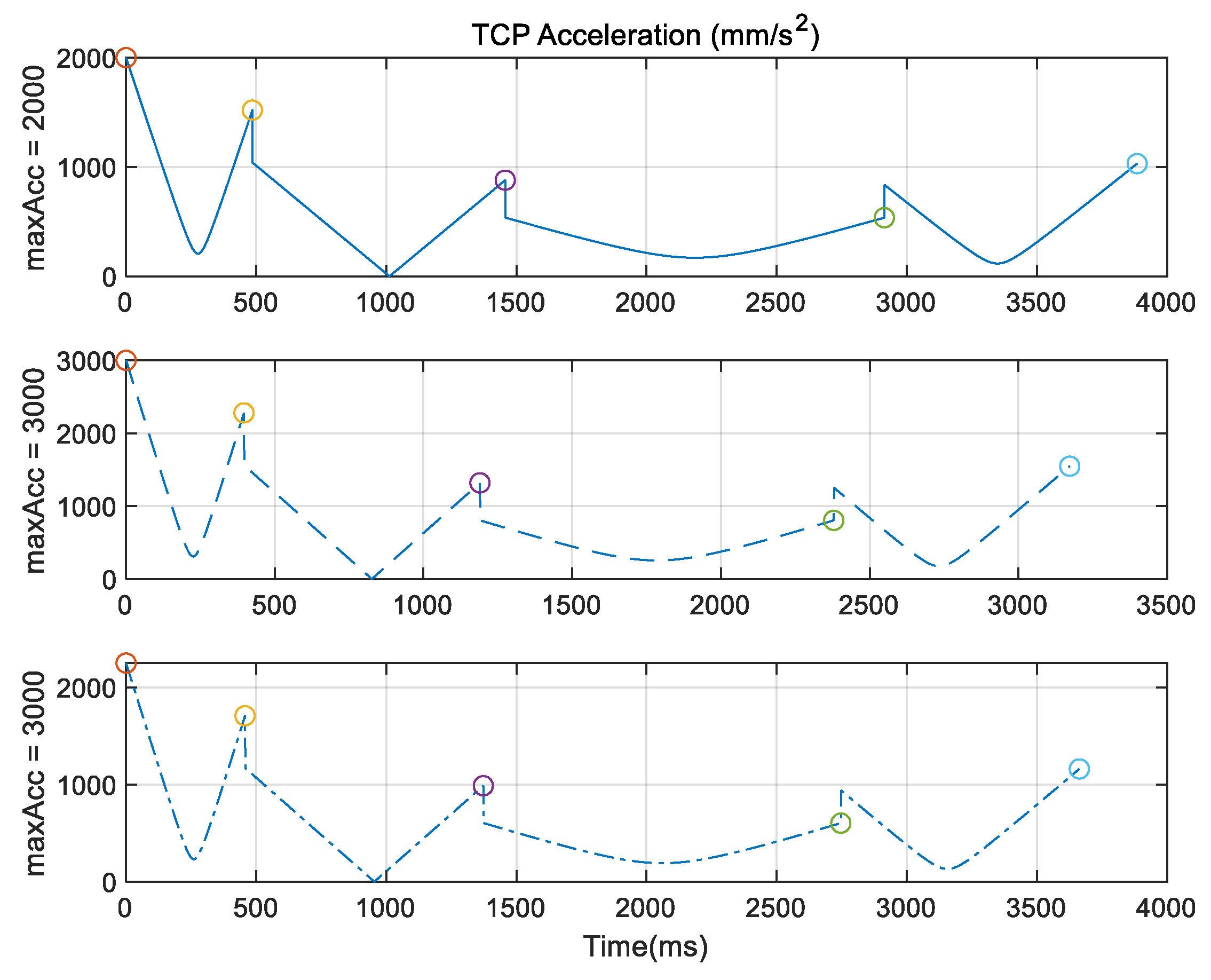
The effect of optimizing the time of motion is evaluated in the simulation with task #2. To evaluate the optimization of the motion time, three cases are compared with the knots in task #2 and is set to 0, as shown in Table 3. The resulting velocity and acceleration are shown in Figure 13 and Figure 14, respectively. In the first case, the maximum velocity is less than 300 . However, the maximum acceleration is 2000 when time is zero and is equal to . The is then changed to 3000 in the second case. Subsequently, the maximum acceleration in the planned trajectory becomes 3000 and motion time is decreased by approximately 0.7 s. This means that motion is optimized by satisfying the acceleration limit. In the third case, is set at 300 to verify the effect of the velocity limit. The third plot in Figure 13 shows that the maximum velocity in the trajectory is equal to , whereas maximum acceleration is less than , as shown in the third plot in Figure 14. This shows that motion is optimized by limiting the maximum velocity of the robot.
4. Experiments in 3-D Industrial Task
4.1. Target Task
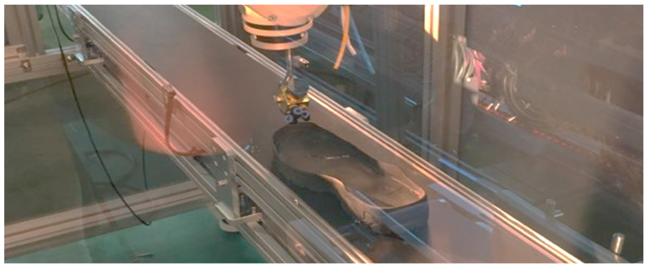
One of the tasks performed at a shoe manufacturing site is attaching a sole to the upper part of a shoe, after dispensing adhesive on the upper contour of the sole. As shown in Figure 15, the robot targets the path generation problem and applies the adhesive evenly to the outer edge of the shoe sole. The generation of spline trajectory is executed based on the point data on the outer path of the sole, which were measured using a 3-D scanner. The target sole is approximately 290, 105, and 25 mm in length, width, and height, respectively.
4.2. Experiment to Validate the Effect on the Number of Points
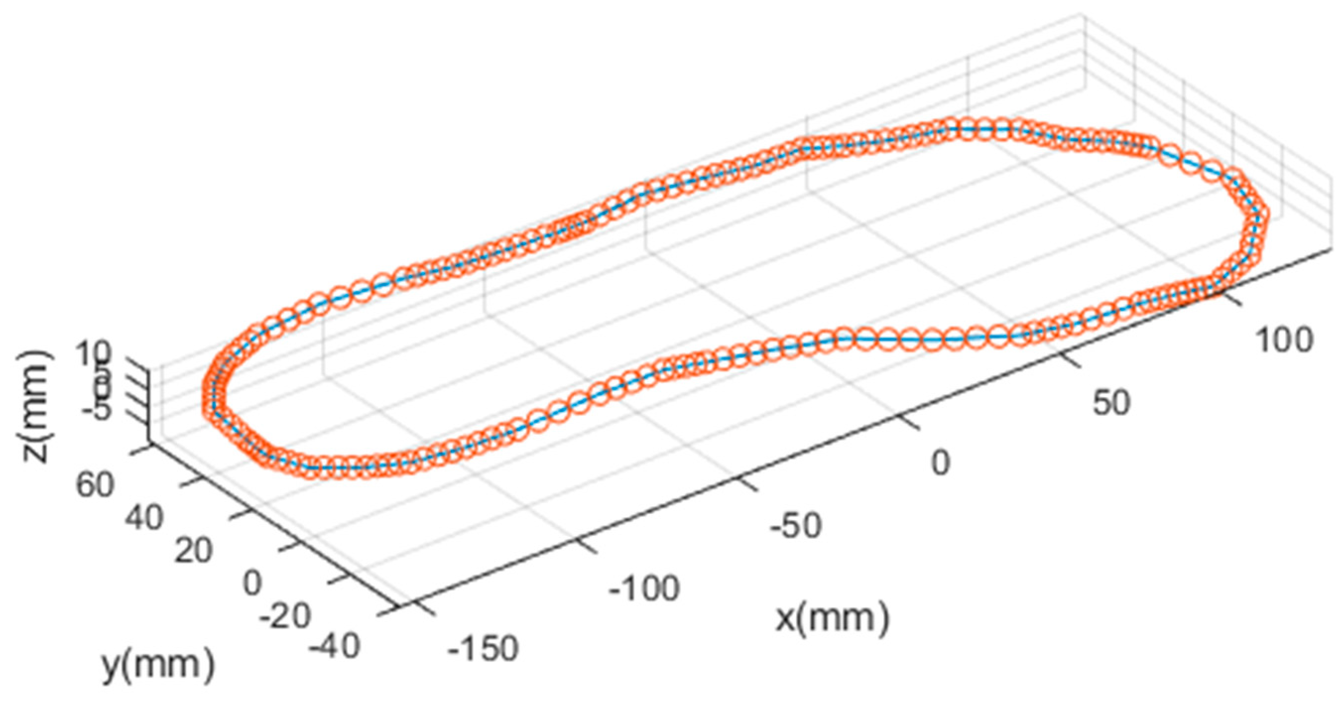
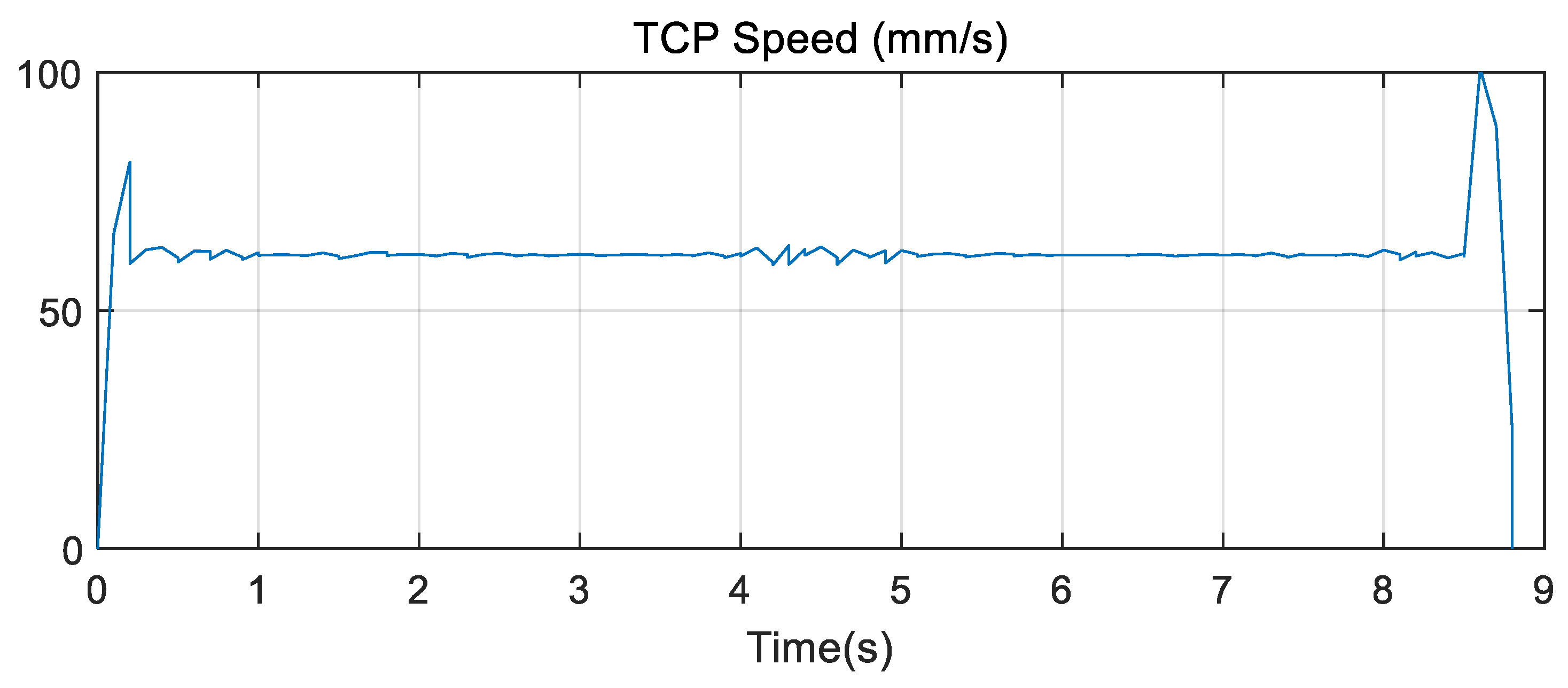
The measured data from the 3-D scanner are the 3-D positions of 169 points, and they are represented as circles in Figure 16. The solid line in Figure 15 is the resulting path that is mapped out based on the proposed spline method. The velocity profile in the trajectory is shown in Figure 17. The initial and final values of the velocity are both zero, consequently, velocity is nearly uniform. To validate the impact on the number of points, the experiment was conducted with a reduced number of points.
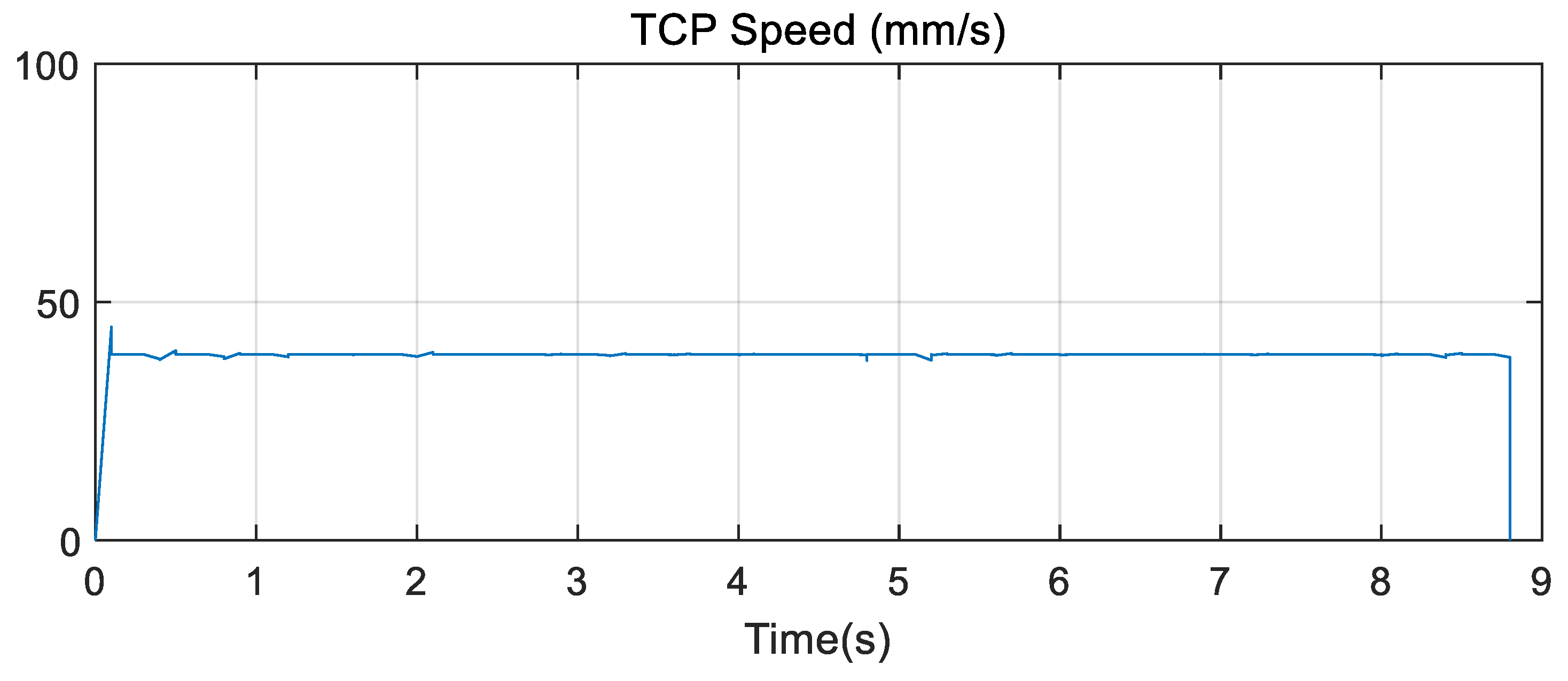
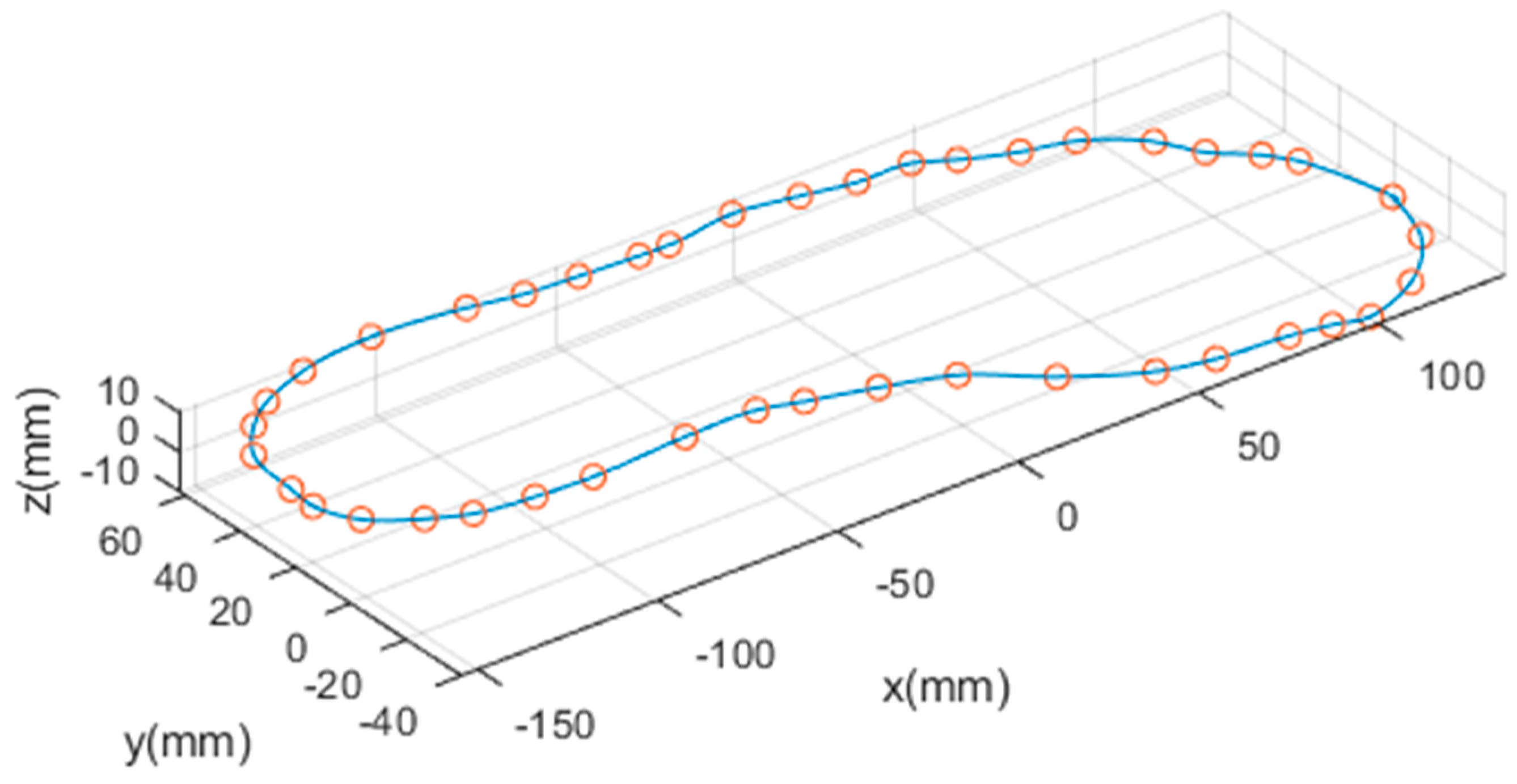
The second test involved planning the trajectory based on reduced point data that were sampled from 262 scanned points. In this case, 43 points were selected and the planned path is illustrated in Figure 18. The overall path appears similar to that in Figure 16. The velocity profile is shown in Figure 19, showing a slight variation when compared with the profile in Figure 16. It is inferred that velocity is relatively uniform because the segment between two neighboring points is sufficiently small in the first case.
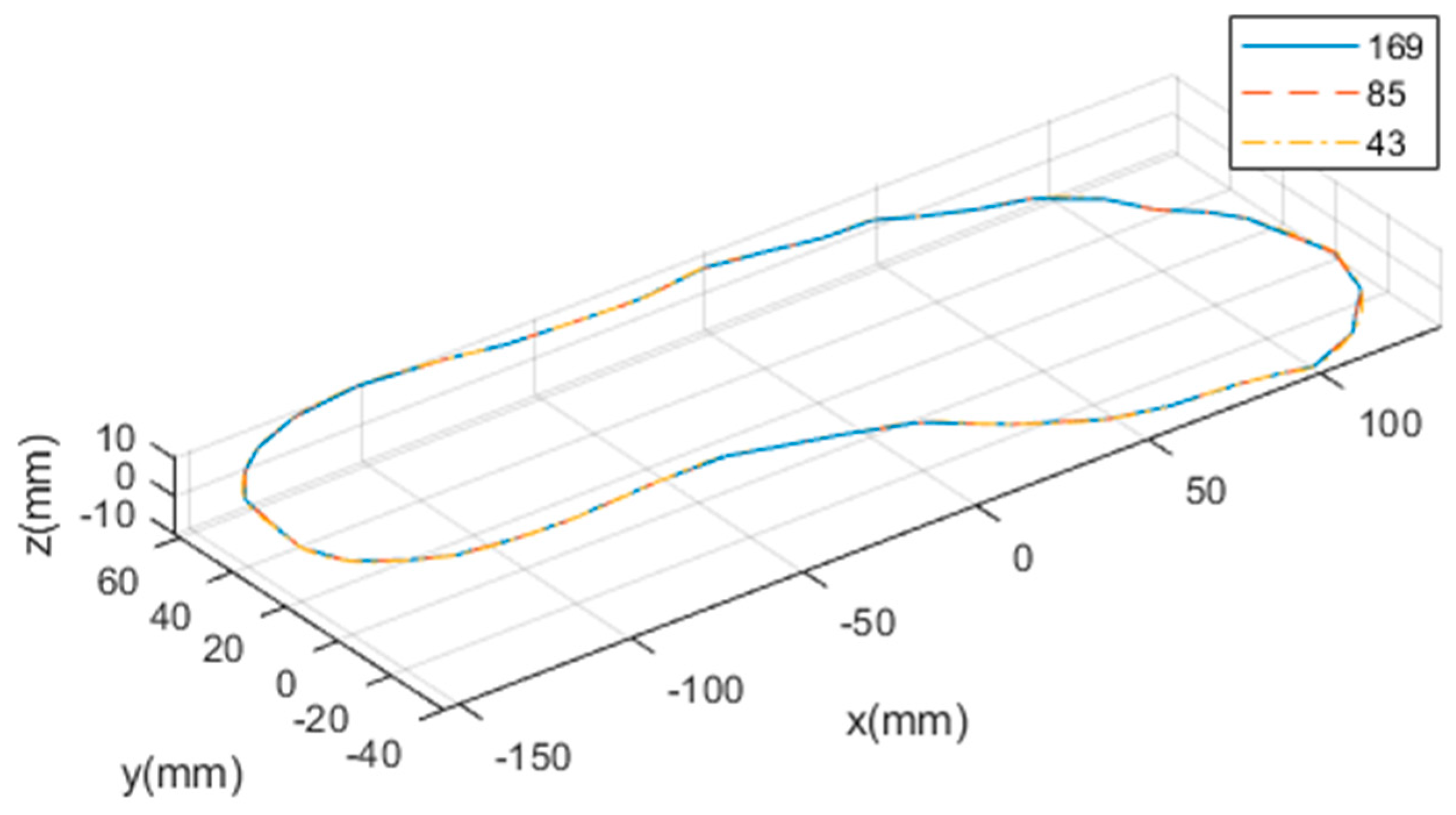
Three paths are shown in Figure 20 to comprehensively compare the planned paths from different numbers of points. The solid and dashed lines are almost the same in the entire path. However, the dotted lines formed when 43 points are used for planning are not matched with the other path in some parts. The maximum positional difference between the case with 169 points and that with 43 points is approximately 2 mm. However, the maximum positional difference between the case with 169 points and that with 85 points is less than 1 mm.
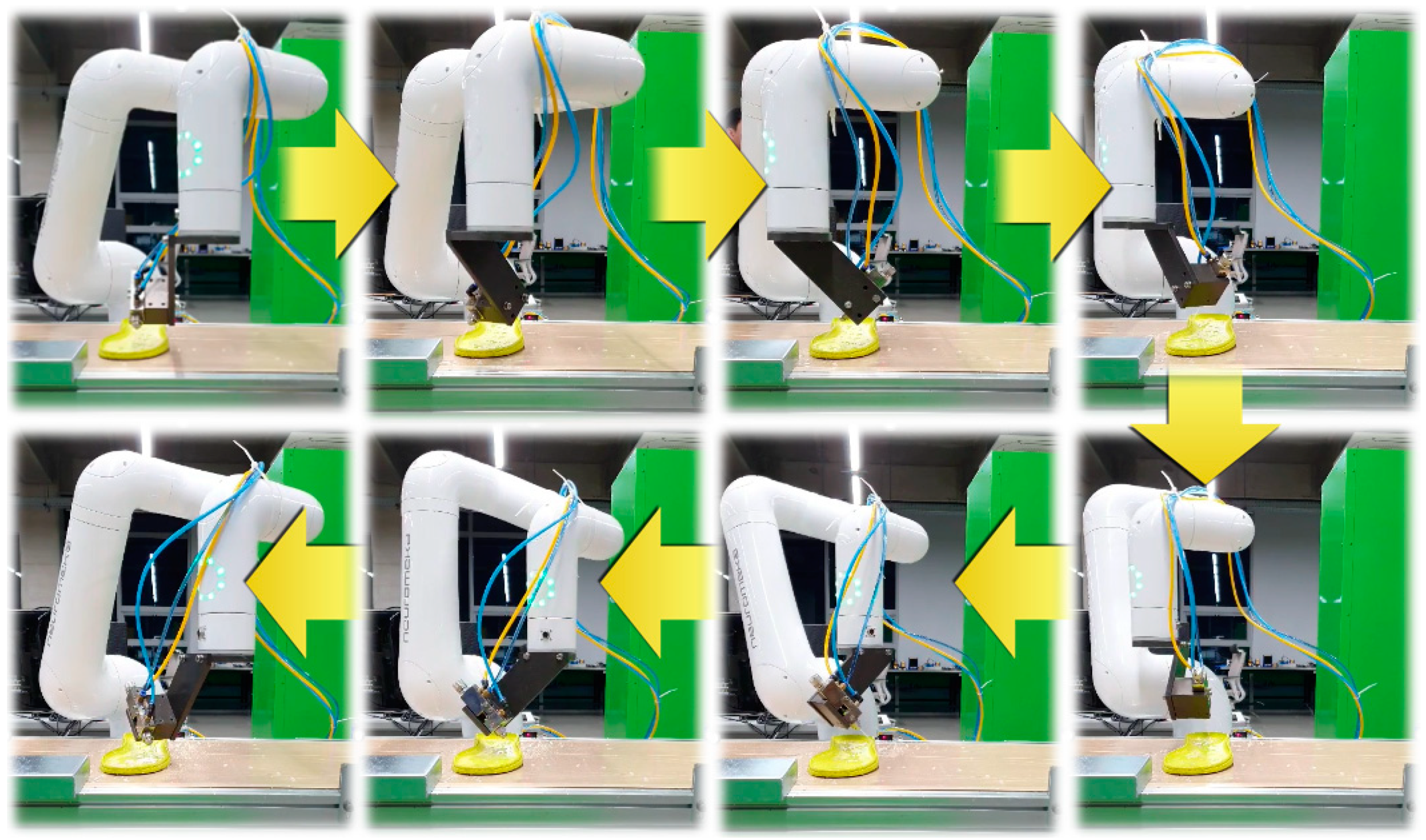
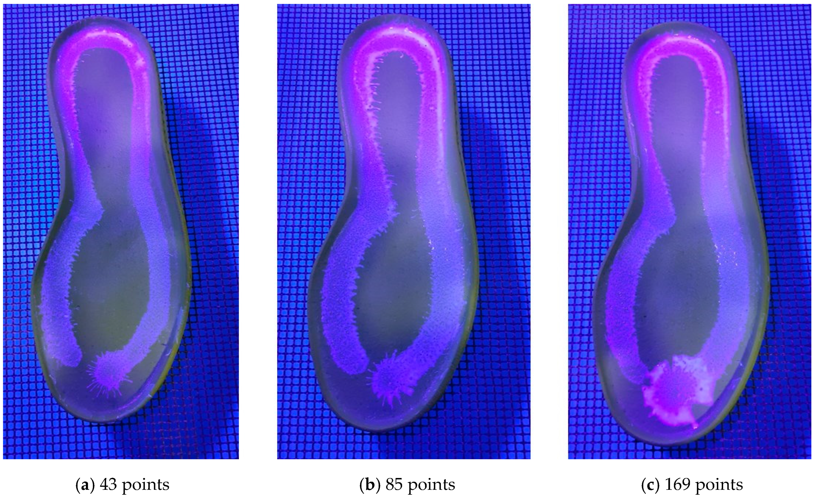
An experiment was implemented to evaluate the proposed spline method and verify that it can be applied to the robotic task in manufacturing sites. The planned trajectory was transferred to the industrial robot with a dispensing tool and the experiment was conducted to check the variation of dispensing qualities according to the number of points. The experimental setup consisted of the glue dispensing tool and the 6-DOF(Degree of Freedom) manipulator, Indy-7, supplied from Neuromeka in Korea as shown in Figure 21. Figure 21 is a snapshot of the scene, where the TCP of the robot performs dispensing. The glue was sprayed through the nozzle at the tip of the dispensing tool while the robot was moving. The color of the glue was transparent. Therefore, the result can be examined through the blue light as shown in Figure 22. Three tests were conducted and the results are shown in Figure 22. It can be shown that glue is well sprayed along the contour of the sole and there is little deviation when three cases are compared. Therefore, the experimental results show that there is not much different depending on the number of points. By considering this result, it is advantageous to take advantage of a small number of points for rapid production.
4.3. Experiment to Validate the Uniform Distribution
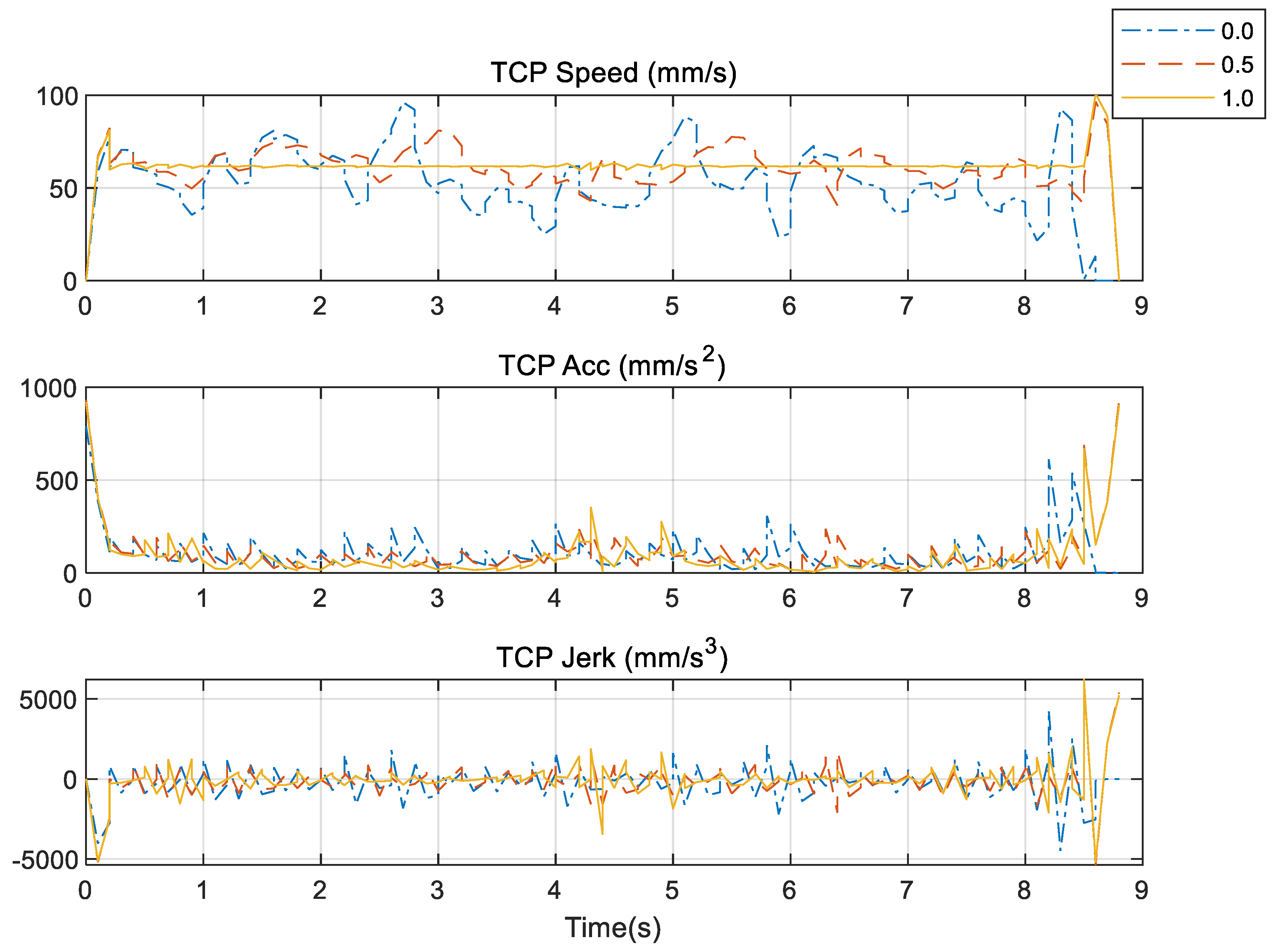
When dispensing adhesives on shoes, the uniform distribution of adhesives is very important, and to satisfy this condition, the operation involving a robot should follow a trajectory that can guarantee the uniform speed of the robot end-effector. The time at each knot is assigned by the chordal case () in Equation (4). Then, the moving time between two neighboring points is made proportional to the distance between these two points. To evaluate and check the effect of the time allocation between knots, the experiments are conducted by changing the value of in Equation (4). The target points are the 3-D positions of 43 points, and they are represented as circles in Figure 18. The three cases depending on the value of were applied and the results of TCP speed, acceleration, and jerks are shown in Figure 23. The solid line in Figure 23 is the resulting trajectory when was set to 1. It is shown that the initial and final values of velocity are both zero, and the TCP speed had uniform value in the entire path.
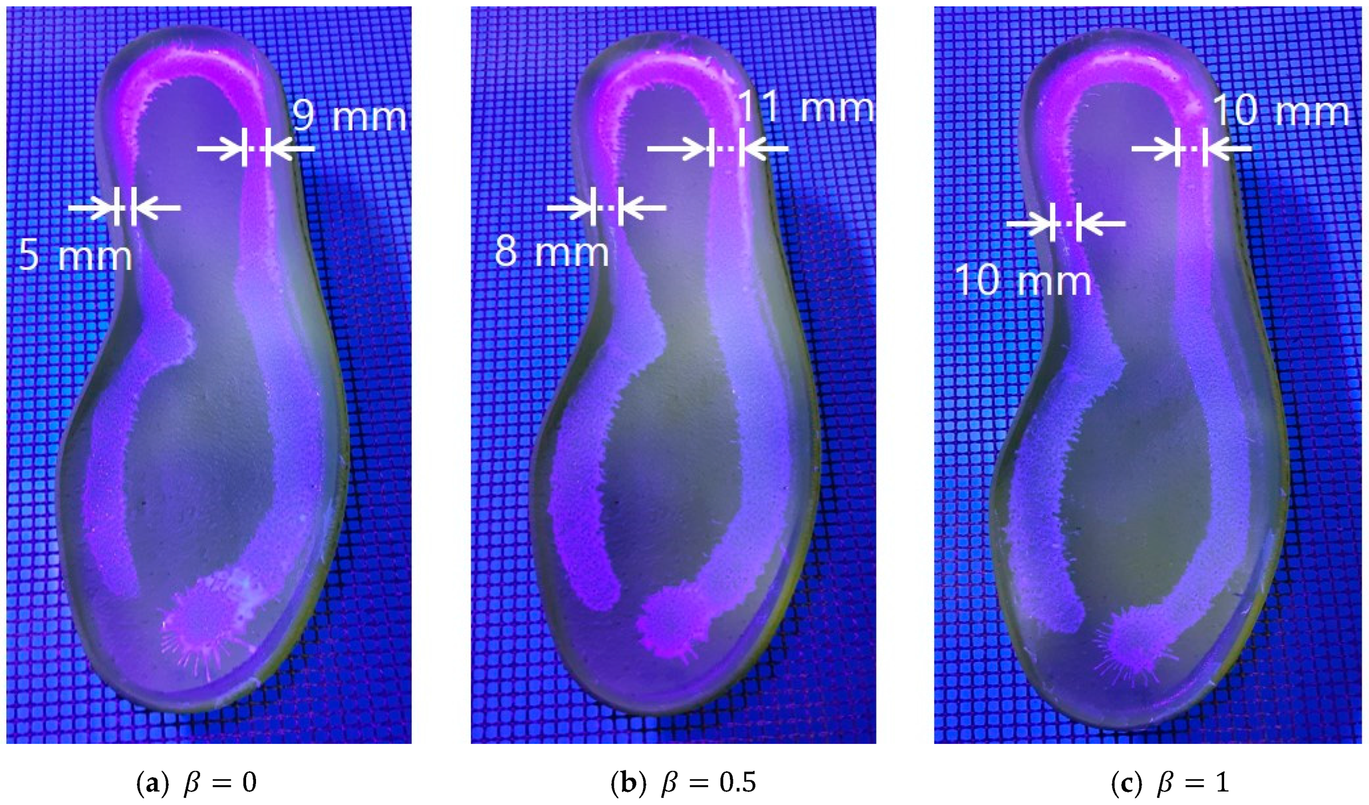
The resultant products are shown in Figure 24. It is verified that the adhesive is evenly dispensed on the desired contour when is 1, as shown in Figure 24c. In the case of Figure 24a when is 0, narrow and non-uniform sections are visible and maximum 4 mm deviation exists in width. Similar results are shown when is 0.5 in Figure 24b. Finally, the experimental results show that the proposed method with timing by the chordal case can generate a spline trajectory for uniform dispensing. The movie for this experiment can be accessed on the website in reference [35].
.
5. Conclusions
In this study, the authors proposed a method for generating the trajectory of a robot using the spline method, which allows the robot to move several points without stopping in a task space. The basic interpolation was based on the Catmull–Rom spline, which satisfied the continuity of velocity at each knot. To adapt a basic Catmull–Rom spline to the robot trajectory planning problem, a method was proposed to select control points outside the trajectory such that the initial and final velocities of the robot were zero. The simulation results demonstrated that the trajectory did not change with respect to time at each knot when the relative distance between two neighboring points was constant for the entire path. However, when the relative distance was varied and the chordal Catmull–Rom spline applied, the robot moved at a relatively uniform speed to execute a spline motion, in which the time in each segment was determined to be proportional to the relative distance between two points.
By proposing the motion time redistribution method based on the maximum velocity and acceleration of the robot, the motion time of the actual robot could be optimized. This was verified via simulations using various maximum velocities and accelerations.
The proposed method is applicable to various robotic tasks requiring a robot to move continuously through multiple assigned points. To evaluate this, an experiment is executed to follow a 3-D curved contour. The target task is for the robot manipulator to dispense adhesive uniformly on the upper contour of the sole at a shoe manufacturing factory. The experimental results show that the proposed trajectory planning in the task space can be applied to the robotic task in the real manufacturing process.
Although the simulation and experimental results demonstrated that the proposed method was applicable to the robotic trajectory problem, this method could not guarantee the continuity of acceleration, and the curvature constraint in the cases where the knots consist of sharp curves should be considered. In the future, this method will be more applied to various complicated robotic tasks, and a method will also be studied to guarantee the continuity of acceleration and the constraints of physical curvature.
Author Contributions
Conceptualization, M.J., S.Y.C., and M.J.H.; Methodology, J.K., S.Y.C., and M.J.H.; Data Curation, J.K., S.H.P., and S.Y.C.; Software, J.K., S.Y.C., and M.J.H.; Experiment, J.K., S.H.P., and M.J.; Analysis, J.K., M.J., S.Y.C., and M.J.H.; Writing—Original Draft Preparation and Revision, J.K., S.Y.C., and M.J.H.; Supervision, S.Y.C. and M.J.H.; Funding Acquisition, M.J. and M.J.H. All authors have read and agreed to the published version of the manuscript.
Funding
This work was supported in part by the National Research Foundation of Korea (NRF) grants funded by the Korean government (MSIT) (No. NRF-2019R1F1A1052895) and in part by the Ministry of Trade, Industry & Energy (MOTIE, Korea) under the Industrial Technology Innovation Program. No. 20001593, “Development of sole manufacturing and assembly system for smart shoe factory”.
Conflicts of Interest
The authors declare no conflict of interest.
References
- Biagiotti, L.; Melchiorri, C. Trajectory Planning for Automatic Machines and Robots, 2nd ed.; Springer: Berlin/Heidelberg, Germany, 2008; pp. 62–76. ISBN 978-3-540-85628-3. [Google Scholar]
- Guan, Y.; Yokoi, K.; Stasse, O.; Khaddar, A. On robotic trajectory planning using polynomial interpolations. In Proceedings of the IEEE International Conference on Robotics and Biomimetics (ROBIO), Shatin, China, 5–9 July 2005; pp. 111–116. [Google Scholar] [CrossRef]
- Available online: http://www.diag.uniroma1.it/~deluca/ (accessed on 31 January 2020).
- Chen, W.; Li, X.; Ge, H.; Wang, L.; Zhang, Y. Trajectory Planning for Spray Painting Robot Based on Point Cloud Slicing Technique. Electronics 2020, 9, 908. [Google Scholar] [CrossRef]
- Lan, J.; Xie, Y.; Liu, G.; Cao, M. A Multi-Objective Trajectory Planning Method for Collaborative Robot. Electronics 2020, 9, 859. [Google Scholar] [CrossRef]
- Mohsin, I.; He, K.; Li, Z.; Du, R. Path Planning under Force Control in Robotic Polishing of the Complex Curved Surfaces. Appl. Sci. 2019, 9, 5489. [Google Scholar] [CrossRef] [Green Version]
- Augustine, J.; Mishra, A.K.; Patra, K. Mathematical Modeling and Trajectory Planning of a 5 Axis Robotic Arm for Welding Applications. In Proceedings of the 3rd International Conference on Production and Industrial Engineering, Jalandhar, India, 29–31 March 2013. [Google Scholar] [CrossRef]
- Park, S.; Lee, M.C.; Kim, J. Trajectory Planning with Collision Avoidance for Redundant Robots Using Jacobian and Artificial Potential Field-based Real-time Inverse Kinematics. Int. J. Control. Autom. Syst. 2020, 18, 2095–2107. [Google Scholar] [CrossRef]
- Cimurs, R.; Suh, I.H. Time-optimized 3D Path Smoothing with Kinematic Constraints. Int. J. Control. Autom. Syst. 2020, 18, 1277–1287. [Google Scholar] [CrossRef]
- Kim, M.; Kim, J.; Shin, D.; Jin, M. Robot-based Shoe Manufacturing System. In Proceedings of the 18th International Conference on Control, Automation and Systems (ICCAS), Daegwallyeong, Korea, 17–20 October 2018; pp. 1491–1494. [Google Scholar]
- Bu, X.; Su, H.; Zou, W.; Wang, P. Curvature continuous path smoothing based on cubic bezier curves for car-like vehicles. In Proceedings of the IEEE International Conference on Robotics and Biomimetics (ROBIO), Zhuhai, China, 6–9 December 2015; pp. 1453–1458. [Google Scholar] [CrossRef]
- Zhu, Z.; Schmerling, E.; Pavone, M. A convex optimization approach to smooth trajectories for motion planning with car-like robots. In Proceedings of the IEEE International Conference on Decision and Control (CDC), Osaka, Japan, 15–18 December 2015; pp. 835–842. [Google Scholar] [CrossRef] [Green Version]
- Wang, X.; Jiang, P.; Li, D.; Sun, T. Curvature Continuous and Bounded Path Planning for Fixed-Wing UAVs. Sensors 2017, 17, 2155. [Google Scholar] [CrossRef]
- Dupac, M. Smooth trajectory generation for rotating extensible manipulators. Math. Methods Appl. Sci. 2018, 41, 2281–2286. [Google Scholar] [CrossRef]
- Pacheco, R.R.; Hounsell, M.S.; Rosso, R.S.U., Jr.; Leal, A.B. Smooth trajectory tracking interpolation on a robot simulator. In Proceedings of the Latin American Robotics Symposium and Intelligent Robotics Meeting, Sao Bernardo do Campo, Brazil, 23–28 October 2010; pp. 13–18. [Google Scholar] [CrossRef]
- Elbanhawi, M.; Simic, M. Sampling-based robot motion planning: A review. IEEE Access 2014, 2, 56–77. [Google Scholar] [CrossRef]
- de Boor, C. A Practical Guide to Splines; Springer: New York, NY, USA, 2001; pp. 40–43. ISBN 0-387-95366-3. [Google Scholar]
- Dyllong, E.; Visioli, A. Planning and real-time modifications of a trajectory using spline techniques. Robotica 2003, 21, 475–482. [Google Scholar] [CrossRef]
- Koch, P.E.; Wang, K. The introduction of B-splines to trajectory planning for manipulators. ModelingIdentif. Control 1988, 9, 69–80. [Google Scholar] [CrossRef] [Green Version]
- Biagiotti, L.; Melchiorri, C. B-spline based filters for multi-point trajectories planning. In Proceedings of the IEEE International Conference on Robotics and Automation (ICRA), Anchorage, AK, USA, 3–7 May 2010; pp. 3065–3070. [Google Scholar] [CrossRef] [Green Version]
- Haron, H.; Rehman, A.; Adi, D.I.S.; Lim, S.P.; Saba, T. Parameterization Method on B-Spline Curve. Math. Probl. Eng. 2012, 640742. [Google Scholar] [CrossRef] [Green Version]
- Xu, Z.; Wei, S.; Wang, N.; Zhang, X. Trajectory Planning with Bezier Curve in Cartesian Space for Industrial Gluing Robot. Lect. Notes Comput. Sci. 2014, 8918, 146–154. [Google Scholar] [CrossRef]
- Kolter, J.Z.; Ng, A.Y. Task-space trajectories via cubic spline optimization. In Proceedings of the IEEE International Conference on Robotics and Automation (ICRA), Kobe, Japan, 12–17 May 2009; pp. 1675–1682. [Google Scholar] [CrossRef] [Green Version]
- Ogniewski, J. Cubic Spline Interpolation in Real-Time Applications using Three Control Points. Comput. Sci. Res. Notes 2019, 1–10. [Google Scholar] [CrossRef]
- Visioli, A. Trajectory planning of robot manipulators by using algebraic and trigonometric splines. Robotica 2000, 18, 611–631. [Google Scholar] [CrossRef]
- Dupac, M. A combined polar and Cartesian piecewise trajectory generation and analysis of a robotic arm. Comput. Math. Methods 2019, 1, e1049. [Google Scholar] [CrossRef] [Green Version]
- Catmull, E.; Rom, R. A class of local interpolating splines. Comput. Aided Geom. Des. 1974, 317–326. [Google Scholar] [CrossRef]
- Yuksel, C.; Schaefer, S.; Keyser, J. Parameterization and applications of Catmull-Rom curves. Comput. Aided Des. 2011, 43, 747–755. [Google Scholar] [CrossRef] [Green Version]
- DeRose, T.D.; Barsky, B.A. Geometric continuity, shape parameters, and geometric constructions for Catmull-Rom splines. ACM Trans. Graph. (TOG) 1988, 7, 1–41. [Google Scholar] [CrossRef] [Green Version]
- Bazaz, S.A.; Tondu, B. Minimum time on-line joint trajectory generator based on low order spline method for industrial manipulators. Robot. Auton. Syst. 1999, 29, 257–268. [Google Scholar] [CrossRef]
- Broquere, X.; Sidobre, D.; Nguyen, K. From motion planning to trajectory control with bounded jerk for service manipulator robots. In Proceedings of the IEEE International Conference on Robotics and Automation (ICRA), Anchorage, AK, USA, 3–7 May 2010; pp. 4505–4510. [Google Scholar] [CrossRef]
- Huang, J.; Hu, P.; Wu, K.; Zeng, M. Optimal time-jerk trajectory planning for industrial robots. Mech. Mach. Theory 2018, 121, 530–544. [Google Scholar] [CrossRef]
- Tondu, B.; Bazaz, S.A. The Three-Cubic Method: An Optimal Online Robot Joint Trajectory Generator under Velocity, Acceleration, and Wandering Constraints. Int. J. Robot. Res. 1999, 18, 893–901. [Google Scholar] [CrossRef]
- Yoon, H.J.; Chung, S.Y.; Kang, H.S.; Hwang, M.J. Trapezoidal Motion Profile to Suppress Residual Vibration of Flexible Object Moved by Robot. Electronics 2019, 8, 30. [Google Scholar] [CrossRef] [Green Version]
- Available online: https://youtu.be/I6UyaKXRmGs (accessed on 20 August 2020).
Figure 1.
Dispensing robot and 3-D scanner in a shoe manufacturing process.

Figure 2.
Concepts of B-, Hermite, and Bezier splines.

Figure 3.
Single path used to connect and using Catmull–Rom spline.

Figure 4.
Path for multiple knots from to .

Figure 5.
Flowchart of process to plan trajectory for multiple knots from to .

Figure 6.
Path for five knots according to in the task #1.

Figure 7.
Velocity and acceleration according to in the task #1. TCP—Tool Center Point.

Figure 8.
Path for five knots according to in the task #2.

Figure 9.
Velocity according to in the task #2.

Figure 10.
Acceleration according to in the task #2.

Figure 11.
Path for five knots in the task #1 when two different methods are applied.

Figure 12.
Path for five knots in the task #2 when two different methods are applied.

Figure 13.
Velocity when assigned maximum velocity is changed.

Figure 14.
Acceleration when assigned maximum acceleration is changed.

Figure 15.
Dispensing glue on contour of sole using robot.

Figure 16.
Scanned points and path mapped out using 169 points.

Figure 17.
TCP speed in the trajectory using 169 points.

Figure 18.
Sampled points and mapped out path using 43 points.

Figure 19.
TCP speed in trajectory planned using 43 points.

Figure 20.
Paths planned using 169, 85, and 43 points.

Figure 21.
Adhesive dispensing test of shoe midsole.

Figure 22.
Test result for adhesive dispensing of shoe midsole depending on the number of the knots.
Figure 22.
Test result for adhesive dispensing of shoe midsole depending on the number of the knots.

Figure 23.
TCP speed, acceleration, and jerk in trajectory planned using 43 points.

Figure 24.
Test result for adhesive dispensing of shoe midsole depending on the value of .


Table 1.
Position (X, Y, Z) in mm of knots.
| knot | Task #1 | Task #2 |
|---|---|---|
| 1 | (0, 0, 0) | (0, 0, 0) |
| 2 | (100, 0, 0) | (100, 0, 0) |
| 3 | (100, 100, 0) | (100, 200, 0) |
| 4 | (200, 100, 0) | (400, 200, 0) |
| 5 | (200, 0, 0) | (400, 0, 0) |
Table 2.
Computation time for the trajectory planning in ms.
| Time | Task #1 | Task #2 | ||
|---|---|---|---|---|
| Catmull–Rom | Cubic | Catmull–Rom | Cubic | |
| Average | 20.7 | 26.6 | 21.8 | 27.1 |
| Standard deviation | 2.8 | 4.1 | 2.7 | 3.9 |
Table 3.
Maximum velocity and acceleration of robot.
| Case | ||
|---|---|---|
| 1 | 1000 | 2000 |
| 2 | 1000 | 3000 |
| 3 | 300 | 3000 |
© 2020 by the authors. Licensee MDPI, Basel, Switzerland. This article is an open access article distributed under the terms and conditions of the Creative Commons Attribution (CC BY) license (http://creativecommons.org/licenses/by/4.0/).
Share and Cite
MDPI and ACS Style
Kim, J.; Jin, M.; Park, S.H.; Chung, S.Y.; Hwang, M.J. Task Space Trajectory Planning for Robot Manipulators to Follow 3-D Curved Contours. Electronics 2020, 9, 1424. https://doi.org/10.3390/electronics9091424
AMA Style
Kim J, Jin M, Park SH, Chung SY, Hwang MJ. Task Space Trajectory Planning for Robot Manipulators to Follow 3-D Curved Contours. Electronics. 2020; 9(9):1424. https://doi.org/10.3390/electronics9091424
Chicago/Turabian StyleKim, Juhyun, Maolin Jin, Sang Hyun Park, Seong Youb Chung, and Myun Joong Hwang. 2020. "Task Space Trajectory Planning for Robot Manipulators to Follow 3-D Curved Contours" Electronics 9, no. 9: 1424. https://doi.org/10.3390/electronics9091424
Note that from the first issue of 2016, this journal uses article numbers instead of page numbers. See further details here.