Series Arc Fault Detection Method Based on Category Recognition and Artificial Neural Network

Abstract

The influence of a series arc on line current is different with different loads, which makes it difficult to accurately extract arc fault characteristics suitable for all loads according to line current signal. To improve the accuracy of arc fault detection, a series arc fault detection method based on category recognition and an artificial neural network is proposed on the basis of analyzing the current characteristics of arc faults under different loads. According to the waveform of current and voltage, the load is divided into three types: Resistive category (Re), resistive-inductive category (RI), and rectifying circuit with a capacitive filter category (RCCF). Based on the wavelet transform, the characteristics of line current in the time domain and frequency domain when the series arc occurs under different types of loads are analyzed, and then the time and frequency indicators are taken as the inputs of the artificial neural network to establish three-layer neural networks corresponding to three types of loads to realize the detection of the series arc fault of lines under different categories of loads. To avoid the neural network falling into a local optimum, the initial weight and threshold of the neural network are optimized by a genetic algorithm, which further improves the accuracy of the neural network in arc identification. The experimental results show that the proposed arc detection method has the advantages of high recognition rate and a simple neural network model.

1. Introduction

Arc faults are an important factor causing electrical fires. At present, many countries have been paying more attention to protection against arc faults and have formulated corresponding product standards. For example, the United States formulated UL1699 [1], the International Electrotechnical Commission formulated IEC62606 [2], and China formulated GB14287.4 [3] and GB/T31143 [4]. The difficulty of arc fault protection lies in the accurate detection of series arc faults. Therefore, in recent years, many scholars have done much research on the accurate detection of series arc faults.

When the arc fault occurs, the current signals of lines with different loads have various time-frequency characteristics [5,6]: The randomness and fluctuation of the current signal increase and the periodicity in the strict definition is lost. There will be a “zero off” phenomenon at the zero crossing point (namely, where the current waveform shows an obvious shoulder phenomenon); in addition, multiple pulse currents may occur within a period, leading to a significant increase in the high-frequency components of current signals.

The pulse current can be considered a singular point in the current signal, and the random high-frequency component of the current signal makes the current signal nonstationary. The wavelet transform has its unique advantages in dealing with the signal containing singularities or nonstationary signals [7]. Therefore, using the wavelet transform to detect arc faults in series has become a hot research area. Current wavelet transform processing methods can be summarized as follows. In a half period or a full period, the mean value, forward difference, standard deviation, effective value and energy value of approximate or detailed signal after current wavelet transform are used as quantitative indicators to identify arc faults [8,9,10,11,12,13,14,15,16,17]. Reference [8] proposed a detection method that takes the average value of reconstructed current signal after wavelet decomposition and the high frequency coefficient of the difference as the indicator. Reference [12] analyzed the energy characteristics of the current frequency band using the db3 wavelet and determined whether an arc fault occurred by comparing the energy ratio of each frequency band. Reference [14] used the discrete wavelet transform to analyze high-frequency current signals. In reference [17], Wavelet parameters are inserted to process the arc current waveform of arc fault, and then the characteristic parameters and frequency range of the current signal are extracted for detection. In addition, there are also some studies on the load voltage and current waveform when the arc faults occur. For example, reference [18] detected the drop mode change signals of voltage and current through wavelet transform and extracted the root mean square of voltage and current as the indicators. These methods are based on the wavelet transform, which can be applied to many categories of loads and improve the reliability of detection. However, the indicator threshold values above are set artificially, and the setting of threshold values lacks flexibility and reliability.

Artificial neural networks (ANNs) have been a research hotspot in the field of artificial intelligence since the 20th century. They have many advantages, such as self-learning and fast search for optimal solutions, and have attracted extensive attention from many scholars. The influence of the artificial setting can be effectively avoided by using an intelligent algorithm to set the threshold of indicators adaptively [19,20,21,22,23,24]. Reference [19] conducted sparse coding of current time-domain signals and trained the fully connected neural network for discrimination. Reference [20] used the discrete wavelet transform to obtain the spectrum characteristics of current data, and then input the values of spectrum energy into the back-propagation neural networks (BPNN) for training. In reference [21], in-class density, standard deviation and sample difference in current frequency domain signals were taken as inputs of the SOM neural network, and particle swarm optimization was used to optimize the weights of the neural network. In reference [22], the current signal was filtered and converted into a grayscale image in chronological order, and then input into the time domain visual convolutional neural network for training. Reference [24] took the Fourier coefficient and small wave characteristic of current signal as the input of the deep neural network. These methods connected the artificial neural network with the time-frequency indicators of arc fault detection and improved the accuracy of arc fault detection to different degrees. However, most of them adopted complex structures with multiple hidden layers, so there are a large number of neurons, and the operations are relatively complicated. As the load types increase, the disadvantages of such methods become increasingly obvious.

In fact, the effect of arc fault on current waveform is different for different loads. Therefore, it is difficult to find uniform characteristics to identify arc faults. For resistive loads, a shoulder characteristic of the line current can be used as a characteristic parameter. However, for some other loads, the line current without an arc fault can also have a shoulder characteristic, such as the diode rectifier circuit or the SCR voltage regulator circuit. Therefore, on the basis of category recognition, the analysis of line current characteristics is beneficial to improving the accuracy of arc fault identification. In recent years, a number of papers have proposed an arc fault detection method based on this idea. For example, Reference [25] proposed a method to extract feature quantities from the first, third, and fifth harmonics of the current for category recognition. These methods can improve the accuracy of arc fault identification through category recognition and can reduce the use of training data compared with the method of arc fault identification after using data training neural network directly. However, the standard of category recognition is easily interfered with by harmonics of the power grid and harmonics of electric appliances when they work normally, so there is room for further optimization.

Based on this idea, this paper proposes a series arc fault detection method based on category recognition and artificial neural network. According to the waveform of voltage and current and their phase relationship, the load is classified into the resistive category (Re), resistive-inductive category (RI), and rectifying circuit with a capacitive filter category (RCCF). Moreover, the classification standard has strong anti-interference ability and is not easily affected by power grid harmonics. Therefore, the characteristic indicators extracted based on the current signal wavelet transform are more representative, which lays a theoretical foundation for greatly simplifying the artificial neural network. For different load categories, the simple “2-5-1” three-layer artificial neural network can produce better results. Experiments show that this method can cover more load types, has higher accuracy of arc fault detection, and can effectively prevent misjudgment.

2. Influence of Arc Fault on Current Signal under Different Loads

When an arc fault occurs in the circuit, the waveform of the current signal changes significantly, and the waveforms of different categories of loads have different characteristics.

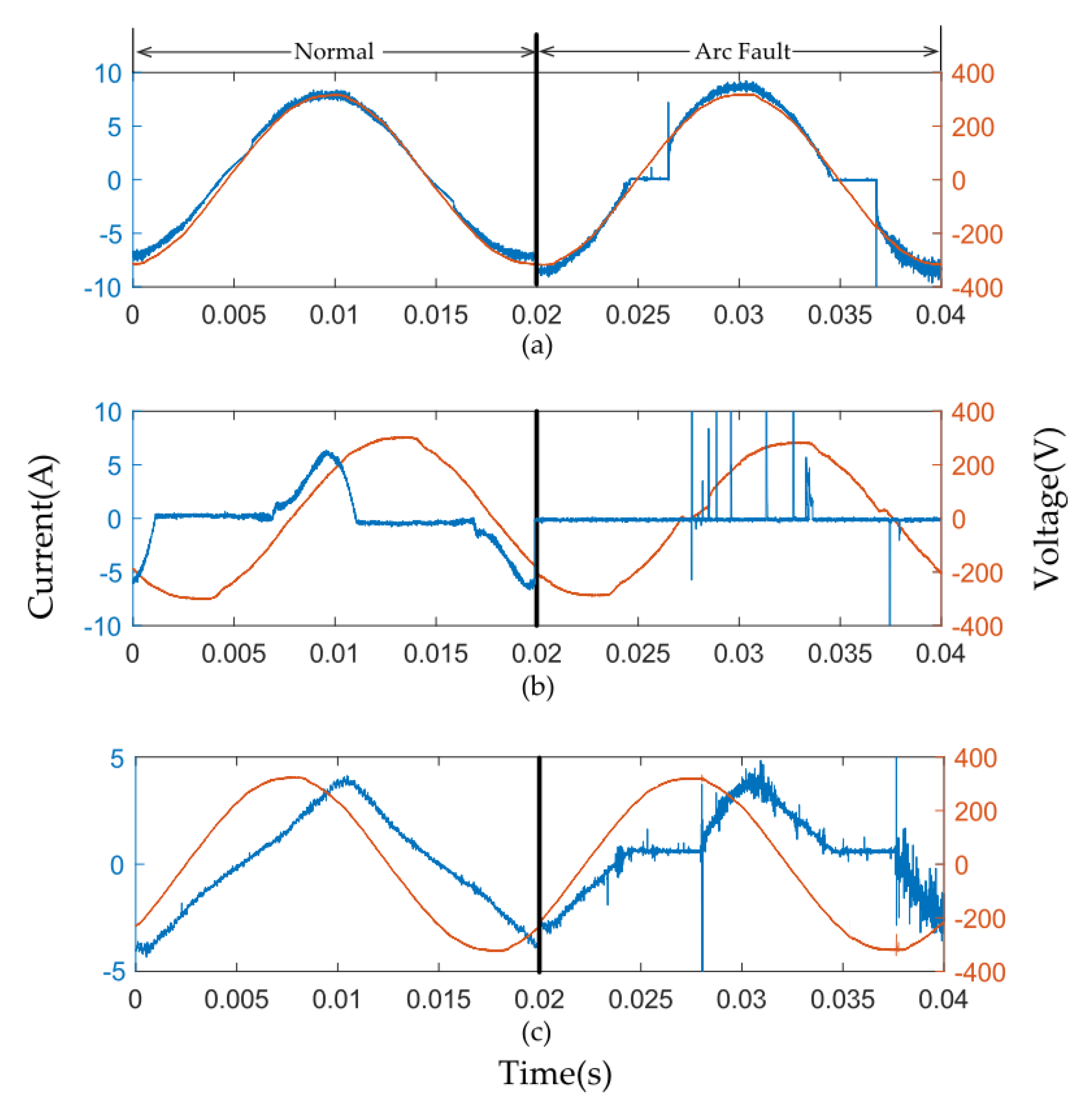
For the resistive category (Re), Figure 1a shows that there is no shoulder in the waveform during the normal state. In the event of a fault, when the arc gap voltage is less than the air gap breakdown voltage, the air is not broken down and the current is zero. When the arc gap voltage exceeds the breakdown voltage, the air is broken down, an arc is generated immediately, the current suddenly changes to a certain numerical value, after which the arc keeps burning, and the current changes with the voltage. When the arc gap voltage is less than the breakdown voltage, the arc extinguishes, the current becomes zero, and the cycle repeats. During the period when the arc gap voltage is less than the breakdown voltage, the current remains at zero; therefore, the current waveform has an obvious shoulder phenomenon at the time of an arc fault.

For the rectifying circuit with a capacitive filter category (RCCF), under normal conditions, when the voltage across the capacitor is lower than the rectifying side voltage, the capacitor is charged, and the current is generated on the power supply side. When the voltage across the capacitor is higher than the rectifying side voltage, the capacitor discharges to the load, and the current of the side of supply power is zero, so there is a shoulder phenomenon during the normal state. To improve the current waveform, such loads are usually added with an inductive filter after the rectifier circuit to slow down the slope when the capacitor is charged. In the fault state, when the arc voltage exceeds the breakdown voltage and an arc is generated, most of the current will charge the capacitor in the load, and the current value will increase rapidly at the moment of charging. At the same time, because the value of the capacitor is generally small, the rising speed of the voltage across the capacitor is higher than the rising speed of the rectifying side voltage, which causes the arc gap voltage to fall rapidly and descend below the breakdown voltage; the arc extinguishes, and the current drops to zero, which is expressed as a pulse current. As the supply voltage rises, the arc gap will be broken down again, the current also appears as a pulse, etc. At this time, there is a certain randomness to whether the diode is turned on. The reason is as follows [26]: Due to the uncertainty of the arc gap distance, the arc extinction voltage is also uncertain under a certain current. After the arc gap is broken, if the arc gap voltage is always greater than the arc extinguishing voltage during the rise of the capacitor voltage, the arc will not extinguish, and the diode will remain turned on. If the arc gap voltage is less than the arc extinguishing voltage, the arc will extinguish, and the diode will not be turned on. Therefore, Figure 1b shows that such a load may have multiple pulse currents in a half period when an arc fault occurs, and the number of pulse currents is not fixed.

For the resistive-inductive category (RI), there is no shoulder phenomenon in the normal state. There is a parasitic capacitance between the turns of the inductive coil of the resistance–inductance load, which can be equivalently connected in parallel with the load. When an arc fault occurs, the arc extinguishes near the zero-crossing time of the current, and the arc gap equivalent resistance is approximately infinite. At this time, the supply voltage will be applied to both ends of the arc gap. The arc gap can only be broken after the arc voltage exceeds the breakdown voltage. The current charges the parasitic capacitance and generates a pulse current (the principle is the same as the RCCF category); that is, when the load is resistive-inductive, pulse currents may occur at the shoulder. The analysis here is consistent with Figure 1c.

The above is a brief summary and analysis of the shoulder phenomenon and mutation phenomenon caused by the arc fault under different categories of loads. In addition, there is a common feature of the above load categories, which is the randomness of the current waveform at the time of an arc fault. During the generation of the arc, the burning of the arc is accompanied by the volatilization of the electrode. The volatilization of the electrode causes the arc gap distance to change, so the arc resistance also changes. According to Ohm’s Law of the whole circuit, when the power supply voltage remains unchanged and the resistance of the arc changes continuously, the current will also fluctuate as shown in Figure 1. If the current is analyzed in the frequency domain, there will be a high frequency noise component, and random characteristics in the frequency domain will be exhibited.

3. Detection Method

The flow of the detection method is shown in Figure 2. This paper will explain each step in accordance with the detection sequence.

3.1. Basis for Dividing the Half Period

The standard of arc fault detection UL1699 requires that when there are more than eight half periods within 0.5 s, the arc fault circuit breaker should perform protection. GB14287.4 requires 14 arcs within 1 s; the detector should issue an alarm signal. GB/T31143 requires that when the line current reaches 75 A, there are 12 half periods of the arc fault within 1 s, and the arc fault protector should be protected by breaking. Using the half period as the time unit to detect whether there is an arc fault that is beneficial to calculating the number of half cycles of the arc existing per unit time, which can better meet the requirements of the related standards.

When an arc fault occurs, the current waveform has the characteristics of randomness and loses periodicity in the strict definition, so the time unit cannot be divided by the current waveform. The waveform of the power supply voltage is almost not affected by the load. Therefore, the time unit can be divided according to the voltage waveform. Figure 3 shows that the period between two adjacent zero-crossing points in the voltage waveform can be divided into a half period.

3.2. Wavelet Transform to Process Signals

The wavelet transform is convenient for detecting the information of sudden points (singular points) in the signal [7]. Therefore, the wavelet transform is used to process the current waveform.

3.2.1. Choosing the Wavelet Base

Daubechies 3 (db3) has a good denoising effect [27]. It is characterized by orthogonality and sensitivity to irregular signal [12]. Therefore, when performing the wavelet transform on the non-stationary signal with much noise information, db3 is suitable for wavelet analysis.

3.2.2. Frequency Band Distribution of the Wavelet Transform

Mallat algorithm is a fast wavelet transform algorithm. Based on the theory of multi-resolution analysis, Mallat proposes the Fast Wavelet Transform (FWT) algorithm, Mallat algorithm [28]. Mallat’s core recursive formulas are shown in Formulas (1) and (2):

$${\overline{a}}_{i+1}(k)={\displaystyle \sum _{j=-\infty }^{\infty }{\overline{a}}_i(j)h(j-2k)}$$

(1)

$${\overline{d}}_{i+1}(k)={\displaystyle \sum _{j=-\infty }^{\infty }{\overline{d}}_i(j)h(j-2k)}$$

(2)

${\overline{a}}_i\left(k\right)$ is the discrete approximation coefficient, ${\overline{d}}_i\left(k\right)$ is the discrete detail coefficient, and h(k) is the filter satisfying the two-scale difference equation.

A previous study found [29] that the frequency range of the current arc is 2–100 kHz, and it is not smooth. Reference [15] found that the amplitude fluctuation of 2.4–39 kHz is more obvious by analyzing the spectrum of different levels after wavelet decomposition. Reference [30], through incandescent lamps, hand drills, fluorescent lamps and other loads, performed spectrum analysis to determine that the high frequency band of the study is below 400 kHz. Therefore, this paper selects 3–100 kHz as the research frequency band; that is, the signal after wavelet transformation should include this frequency band.

To obtain the detailed signal and approximate signal of each layer of decomposition according to the discrete coefficients of wavelet decomposition ${\overline{a}}_i\left(k\right)$ and ${\overline{d}}_i\left(k\right)$ reconstruction, the frequency ranges of the two types of signals are:

$$\{\begin{array}{l}{d}_i(k):[2^{-(i+1)}{f}_s,2^{-i}{f}_s]\\ a_i(k):[0,2^{-(i+1)}{f}_s]\end{array}$$

(3)

$f_s$ is the sampling frequency. Taking the sampling frequency of 200 kHz as an example, the frequency band and spectrum of each layer of wavelet decomposition are shown in

Table 1. Wavelet decomposition frequency segment.

Layer Number	Approximate Signal Concentration Frequency Band (kHz)		Detail Signal Concentration Frequency Band (kHz)
1	a1	0–50	d1	50–100
2	a2	0–25	d2	25–50
3	a3	0–12.5	d3	12.5–25
4	a4	0–6.25	d4	6.25–12.5
5	a5	0–3.125	d5	3.125–6.25

and Figure 2 and Figure 3, respectively. According to the research frequency band, the number of decomposition layers of wavelet transform is determined as five layers.

Figure 4 and Figure 5 show that, after the original signal is decomposed and reconstructed, the amplitude of the approximate signal is much greater than the detailed signal. In addition, the frequency spectrum of the detailed signal of the first layer is concentrated at 50–100 kHz, and the frequency spectrum of the approximate signal is concentrated within 50 kHz. The frequency spectrum of the detailed signal of the second layer is concentrated at 25–50 kHz, and the frequency spectrum of the approximate signal is concentrated within 25 kHz, etc., consistent with the theoretical frequency band distribution presented in Table 1.

As the frequency band of the signal decreases, the noise content decreases, and the waveform backbone becomes clear. Table 1 shows that the fifth layer approximate signal (a5) has the lowest frequency. In addition, Figure 6 shows that after wavelet decomposition, the waveform backbone of the a5 signal is more obvious than that of the original signal, reducing the influence of the interference signal.

In summary, after the original signal is decomposed and reconstructed by the wavelet transform, two different signals are generated: The detailed signal allows focus on the time-frequency characteristics of the waveform and can be used to detect whether the current signal contains a pulse mutation or high-frequency components; the approximate signal can effectively filter out the interference signal and keep the waveform backbone of current, which is convenient to calculate the current indicator such as the “shoulder proportion”.

3.3. Category Recognition

3.3.1. Primary Classification

According to the analysis in Section 2, under the normal state, the current waveforms of the resistive category and the resistive inductive category have no shoulder characteristics. The current waveforms of the rectifying circuit with a capacitive filter category has a shoulder characteristic. Therefore, the load category is divided into two types: Normal with shoulder and normal without shoulder.

By performing wavelet decomposition and reconstruction on the current waveform when various loads are normal, the fifth layer approximate signal a5 is selected to calculate the shoulder ratio of the current signal.

The shoulder always occurs near the zero-crossing point of the current, and the amplitude x_mid about the shoulder is roughly determined as:

$$x_{mid}=\frac{x_{max}+x_{min}}{2}$$

(4)

x_max, x_min are the maximum and minimum currents in a half cycle of power frequency, respectively.

To generalize the results, it is necessary to determine the detection bandwidth of the shoulder: On the basis of mid, the up and down fluctuation does not exceed 5% of the amplitude. Points within this range are considered shoulder points:

$$[x_{mid}-(x_{max}-x_{min})\times 0.05]\le \widehat{x}\le [x_{mid}+(x_{max}-x_{min})\times 0.05]$$

(5)

$$\epsilon =\frac{\mathrm{the} \mathrm{number} \mathrm{of} \widehat{x}}{\mathrm{n}}\times 100\%$$

(6)

n is the number of sampling points in a half cycle of power frequency, and $\epsilon$ is the “shoulder proportion”.

For the three categories of loads, 100 sets of data under normal condition are selected respectively to calculate the proportion of shoulder.

The load examples in Figure 7 show that the loads can be divided into two types (normal with shoulder and normal without shoulder) when thresholds are selected from 4% to 42%. In order to leave a certain margin, the threshold is set as 10%:

$$\begin{array}{l}\epsilon \ge 10\%—\mathrm{normal} \mathrm{with} \mathrm{shoulder}\\ \epsilon <10\%—\mathrm{normal} \mathrm{without} \mathrm{shoulder}\end{array}$$

(7)

3.3.2. Secondary Classification

For a normal load type without shoulder, the voltage and current of the resistive category are in the same phase, and the voltage of the resistive-inductive category leads the current. Therefore, this can be further classified by the phase relationship of the voltage and current signals.

The maximum value of the voltage signal and the current signal within a certain half period are selected to compare the time sequence of the difference between the two:

$$\Delta =\frac{|m_{\mathrm{umax}}-m_{\mathrm{imax}}|}{\mathrm{n}}$$

(8)

n is the number of sampling points in the half cycle of the power frequency, and m is the maximum sampling point label, $\Delta$ is the “phase difference”.

For the loads without shoulder under normal condition, 100 sets of data are also selected respectively to calculate the phase difference.

The load examples in Figure 8 show that the loads can be divided into two types (resistive-inductive category and the resistive category) when thresholds are selected from 1% to 17%. In order to leave a certain margin, the threshold is set as 10%:

$$\begin{array}{l}\Delta \ge 10\%,\mathrm{RI}\\ \Delta <10\%,\mathrm{Re}\end{array}$$

(9)

The load can be classified according to the above classification criteria, as shown in

Table 2. Category recognition.

Primary Classification	Secondary Classification
Normal without shoulder	Resistive category (Re)
	Resistive-inductive category (RI)
Normal with shoulder	Rectifying circuit with a capacitive filter category (RCCF)

.

3.4. Time-Frequency Indicators Selection

Comprehensive use of multiple time-frequency indicators will be more convincing and reliable. In terms of resistive category (Re), the current shoulder ratio increases significantly when arc faults occur. Therefore, “shoulder proportion” is selected as the time domain indicator. In addition, the current of the resistive-inductive category (RI) and rectifying circuit with a capacitive filter category (RCCF) will show more current pulses during faults. Thus, “degree of fluctuation” is quantified. For the frequency domain indicator, the current of all load categories will have a phenomenon of increasing high-frequency components during the fault, and “average energy” is selected to quantify.

The selected indicators are shown in

Table 3. Selection of load indicators and comparison of characteristics.

Category	Time Domain Indicator	Frequency Domain Indicator
Re	Shoulder proportion	Average energy
RI	Degree of fluctuation
RCCF

. The selection methods of the “effective value of the current”, “degree of fluctuation”, and “average energy” are described as follows.

3.4.1. Effective Value of the Current

By calculating the root-mean-square of the approximate signal a5 after wavelet decomposition and reconstruction of the current signal, the effective value of the current is obtained:

$$\alpha =\sqrt{\frac{x_1{}^2+x_2{}^2+x_3{}^2+\dots +x_{\mathrm{n}}{}^2}{\mathrm{n}}}$$

(10)

x is the data column, $\alpha$ is the effective value, and n is the number of sampling points in a half cycle of power frequency.

3.4.2. Degree of Fluctuation

The forward differential of the current a5 signal after wavelet reconstruction is:

$$\begin{array}{l}z(i)=x(i+1)-x(i)\\ (i=1\dots n-1)\end{array}$$

(11)

Then, the differential series is summed to reflect the relativity of the current fluctuation and then divided by the effective value of the current signal half cycle to obtain the fluctuation degree:

$$\gamma =\frac{{\displaystyle \sum _{i=1}^{\mathrm{n}-1}|z(i)|}}{\alpha }$$

(12)

z is the differentiated data, $\gamma$ is the degree of fluctuation, and $\alpha$ is the effective value.

3.4.3. Average Energy

Table 1 shows that the detailed signal is more suitable for analyzing the high-frequency characteristics of current signal when a fault occurs. In addition, the load examples in Figure 9, Figure 10 and Figure 11 show that, after wavelet decomposition, the amplitude of each layer of the five-layer detailed signal of the load is greater than that of the normal time.

Synthesizing the five layers of detailed information of wavelet decomposition, the “average energy” is selected as the frequency domain indicator of all loads. That is, after the decomposition of the five layers of the wavelet, the energies of the detailed signals d₁, d₂, d₃, d₄, and d₅ of different layers are averaged:

$$\eta =\frac{{\displaystyle \sum _{i=1}^{\mathrm{n}}{\mathrm{d}}_1{(i)}^2+{\mathrm{d}}_2{(i)}^2+{\mathrm{d}}_3{(i)}^2+{\mathrm{d}}_4{(i)}^2+{\mathrm{d}}_5{(i)}^2}}{\mathrm{n}}$$

(13)

$\eta$ is average energy, ${\mathrm{d}}_{\mathrm{n}}$ is the layer n of the detailed signal, and n is the number of sampling points in a half cycle of power frequency.

3.5. Construction and Optimization of an Artificial Neural Network

3.5.1. Establishing the BP Neural Network

After the current waveform of the load is quantified by the indicators, it can be further identified by setting a threshold. However, if the thresholds of multiple indicators for different loads and the weights between different indicators are artificially set, since the indicators will randomly fluctuate, this can easily lead to misjudgment. Therefore, artificial neural networks are used to adaptively find the optimal thresholds and weights.

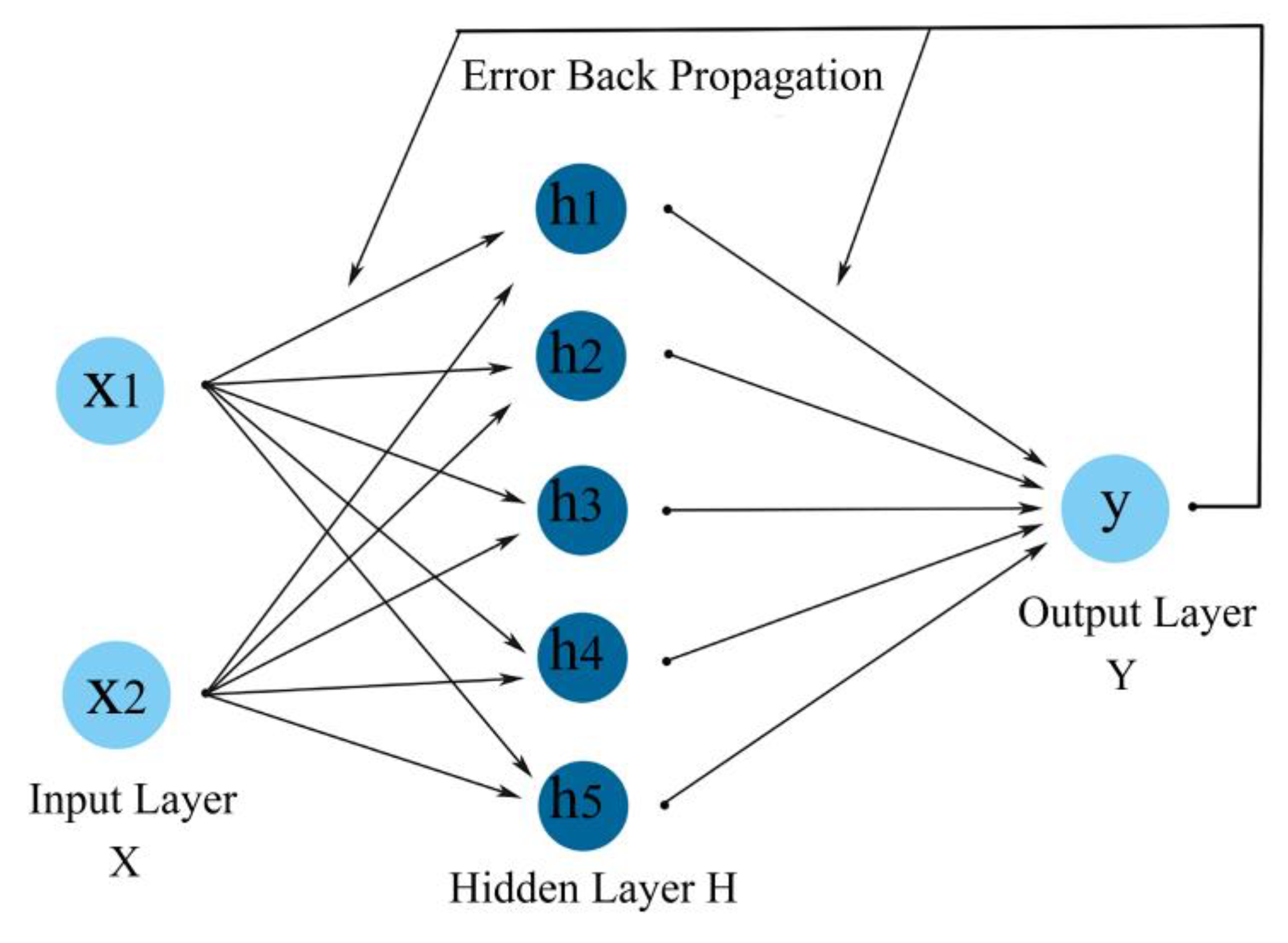
The error back propagation neural network (BP neural network) is a multilayer feedforward neural network. The basic idea is to use the gradient search technique to continuously modify the weights and thresholds between layers to minimize the error between the actual output value of the network and the expected output value [31]. In this paper, a more accurate and reasonable category recognition is carried out, and obvious characteristic indicators are found for each load category, which lays a theoretical foundation for the simplification of artificial neural networks. Therefore, the three-layer BP neural network of “input layer-hidden layer-output layer”, as shown in Figure 12, is used for various load categories.

The BP neural network has a strong multivariate mapping ability and can be used for binary pattern recognition. According to Table 3, this paper takes the time-frequency indicators of different loads as the input of this type of load neural network; the results of identifying the arc fault adopt the binary output of “arc fault 1” and “normal operation 0”, so the number of neurons in the input layer(m₁) is 2, and the number of neurons in the output layer(m₂) is 1. The number of hidden layer neurons can be determined according to the empirical formula:

$$m_2{=2\times m}_1+1=5$$

(14)

There are many types of training kernel functions for BP neural networks. To meet the needs of binary 0–1 output, the transfer function of hidden layer neurons uses the S-type tangent function Tansig, and the transfer function of output layer neurons uses the S-type logarithmic function Logsig. The training kernel function selects the Trainlm function based on the Levenberg-Marquardt algorithm.

The data used to train the network should be normalized in advance, and the data column should be normalized to the interval [0,1] to eliminate the influence of the order of magnitude and unit. The normalization method used in this paper is the maximum-minimum method:

$$x_{kh}=\frac{x_k-{x^{\prime }}_{\mathit{min}}}{{x^{\prime }}_{\mathit{max}}-{x^{\prime }}_{\mathit{min}}}$$

(15)

$x_{\mathit{min}}$ is the minimum value of the data, $x_{\mathit{max}}$ is the maximum value of the data, and $x_h$ is the normalized value of the data.

According to the load category, the BP neural network builds three structures as “2-5-1”. Using the normalized data to train the network, the output of neurons in the output layer is in the range of [0,1]. To generalize the training results, the output values y is organized as follows:

$$y=\{\begin{array}{l}0,(y<0.5,\mathrm{normal})\\ 1,(y\ge 0.5,\mathrm{arcing})\end{array}$$

(16)

3.5.2. Genetic Algorithm Optimized Neural Network

For BP, the neural network is based on the gradient information of error function, when the initial value is not selected properly or the gradient information is hard to get, the BP neural network may be helpless. Before officially training the BP neural network, the genetic algorithm is used to find the optimal initial value, which can improve the performance of the neural network [32]. The algorithm flow [33] is shown in Figure 13:

The “2-5-1” network adopted in this paper has a total of $2\times 5+5\times 1=15$ weights and $5+1=6$ thresholds, and the number of parameters to be optimized is $15+6=21$. Each parameter uses 10-bit binary coding, so the length of the individual in the genetic algorithm is 210 bits. The norm of the error of the test sample is used as an indicator to measure the quality of the network, and the individual’s fitness value is calculated by the error norm. The larger the individual’s fitness value, the better the individual.

The other parameters of the genetic algorithm are shown in

Table 4. Genetic algorithm parameter settings.

Population Size	Genetic Algebra	Mutation Probability	Crossover Probability	Generation Gap
20	50	0.01	0.7	0.95

.

Therefore, BP neural networks optimized by GA (GA-BP networks) of the resistive category, resistive-inductive category, and rectifying circuit with a capacitive filter category were established.

4. Experimental Verification

4.1. Experimental Device and Experimental Object Selection

According to the UL1699 standard of the American arc fault circuit breaker, the arc fault generating device was independently built in the laboratory.

Figure 14a shows the laboratory test platform. The digital oscilloscope model is a Tektronix DPO3054. A TCP0030 current probe is used for current signal acquisition, and a P5200A/50 MHz high-voltage differential probe is used to collect the voltage signals. The arc generator consists of a stationary electrode and a moving electrode; one electrode is a carbon-graphite rod and the other electrode is a copper rod. As shown in Figure 14b, by adjusting the stepping motor, adjusting the distance between the copper rod and the carbon rod to generate an arc, the input voltage is 220 V. Current waveforms during the normal state and under an arc fault state are recorded with an oscilloscope (the sampling frequency is 200 kHz).

Several loads are randomly selected as the test objects, as shown in

Table 5. Experimental loads and their categories.

Experimental Load	Category
Pure resistance (15 Ω) Fluorescent lamp (80 W in total) Halogen lamp (300 W)	Resistive category (Re)
Electric drill (600 W)	Resistive-inductive category (RI)
Air conditioner (4500 W) Computer host (two sets of 500 W in total) Tungsten filament lamp (conduction angle 60°)	Rectifying circuit with a capacitive filter category (RCCF)

. The current waveforms of the load measured in the laboratory under the normal state and fault state are shown in Figure 15, which shows that after the series arc occurs, different categories of load current waveforms show different characteristics, which is consistent with the previous theory.

4.2. Category Recognition Results

Category recognition is performed before using GA-BP neural networks for detection. According to the classification method described in Section 3.3, category recognition of the sample data, the results are shown in

Table 6. Category recognition results.

Category	Number of Samples	Classification Accuracy%
Re	210	100%
RI	210	100%
RCCF	210	100%
Total	630	100%

:

Category recognition is based on the voltage waveforms and current waveforms under normal situation. For different categories of loads, the waveforms vary greatly as shown in Figure 1. Therefore, category recognition is easy to achieve a high accuracy. As Table 6 shows, a total of 630 sets of data were used in the category recognition test, which achieved a high accuracy rate.

4.3. Fault Arc Identification Results

There are currently no generally accepted mathematical rules regarding the division of data sets for the development of artificial neural networks. Only some empirical rules divide the collected data into training sets, test sets, and validation sets, or training sets and test sets [34]. Generally, the ratio of the training set to the test set is roughly 7:3; for example, reference [35] recommended that 65% of the data be used to train the neural network and 35% of the data should be used for test verification. Therefore, for each load category, this paper selects 70% of the data as training samples and 30% of the data as test samples.

The time-frequency indicators of various loads in the training samples according to Table 3 are calculated, and the corresponding neural network is trained. Then, the 630 sets of test samples are tested one by one according to the arc fault detection method shown in Figure 2.

The experimental results are shown in

Table 7. Fault arc identification results.

Load Categories		Training Samples 70%			Test Samples 30%			Comprehensive Accuracy
		Normal Group	Arc Group	Total	Normal Group	Arc Group	Total	BP Networks	GA-BP Networks
Re	Pure resistance	75	75	450	30	30	180	90.79% 1 ~ 93.65%	99.21%
	Fluorescent lamp
	Halogen lamp
RCCF	Air conditioner	75	75		30	30
	Computer host
	Tungsten Filament lamp (with dimmer)
RI	Electric drill	75	75		30	30

¹ The back propagation (BP) networks’ accuracy will fluctuate for multiple trainings with the same data.

, which demonstrates that the method proposed in this paper can efficiently identify the generation of arcs. The comprehensive accuracy of the BP networks fluctuates between 90.79% (572 out of 630 tests) and 93.65% (590 out of 630 tests). At the same time, the recognition accuracy of the GA-BP neural networks is 99.21% (625 out of 630 tests), which proves that the genetic algorithm can effectively improve the recognition accuracy of the neural network for arc generation.

The accuracy of the not optimized neural networks will fluctuate because the initial threshold and weight of the BP neural network are random numbers, so it can easily to fall into a local optimum during the training process. The weight and threshold obtained at this time are not the most appropriate parameters, leading to a decrease in accuracy. Before the BP neural network training, the genetic algorithm is used to find the optimal initial value, which can avoid this problem. Next, through the BP neural network training, the global optimal threshold and weight can be obtained, so the accuracy of the GA-BP neural networks will remain constant. In addition, Figure 16 shows that the comprehensive recognition results of the GA-BP neural networks are relatively concentrated, while the comprehensive recognition results of the BP neural networks are relatively dispersed. Therefore, the use of the genetic algorithm to optimize the BP neural network has a significant effect on improving the stability of accuracy.

5. Comparison with Previous Detection Methods

Starting from the four major aspects of the category recognition method, neural network structure, optimization of the neural network and detection accuracy of arc recognition, the similarities and differences of the four representative methods previously mentioned and the methods proposed in this paper are compared.

Table 8. Comparison of detection methods.

	Reference [25]	Reference [21]	Reference [24]	Test Method in This Paper
Method framework	Select the 1st, 3rd, and 5th harmonics to extract the frequency domain feature quantities for category recognition, combine the time domain feature values to train a fully connected neural network	Extract frequency domain indicators, train SOM neural network	Use Fourier coefficients and wavelet eigenvalues as input for deep neural networks	Two-level category recognition based on current and voltage waveforms, combine wavelet transform to extract time-frequency eigenvalues, train BP neural network
Recognition standard	Extract feature quantity from 1.3.5 harmonic	Not mentioned	Not mentioned	The relationship of load current, voltage waveform, and current waveform
Recognition category	RE, CI, SW			Re, RI, RCCF
Neural network structure	4-5-5-2, 2-5-5-4, 5-12-12-4	49-36-10	607-16-32-16-1	2-5-1
Neural network optimization	Not mentioned	Use particle swarm optimization to optimize initial value of neural network	Not mentioned	Use genetic algorithm to optimize initial value of neural network
Detection accuracy	99.00%	95.00%	95.61%	99.21%

shows that, in terms of category recognition method, the recognition standards of reference [25] are susceptible to interference from grid harmonics and can only be established under certain circumstances. The recognition standards mentioned in this paper are not subject to harmonics interference. It is simple and easy to implement; in terms of neural network structure, this paper greatly simplifies the neural network on the basis of category recognition. There is only one hidden layer, there are two input neurons and one output neuron, and the three neural networks after category recognition have the same structure. In terms of neural network optimization, this paper uses genetic algorithms to optimize the initial value of the network. Compared with other methods, it ensures that the recognition accuracy is stable. In terms of the accuracy of arc detection, the method proposed in this paper is based on category recognition and a simplified network structure, achieving 99.21% accuracy, and the test data includes various load categories, making the results more general and reliable.

In addition, the software accuracy top limitation in the GA-BP is the amount and type of training data. If the type and amount of training data are increased, the accuracy will be further improved. However, training time will also increase.

It should be noted that the focus of this paper is to propose a detection method. Based on the measured data, MATLAB is used to run the algorithm program on the laptop. The CPU of the laptop is Intel(R) Core(TM) i5-6300HQ [email protected]. In addition, as

Table 9. The time required for the detection method.

Category of GA-BP Network	Training Time(s)	Running Time of Detection Function(s)
Re	372.34	0.009
RI	382.36	0.011
RCCF	403.23	0.010

shows, the training time of GA-BP network is less than 403.23 s, and the running time of the detection function is less than 0.011 s. In practice, if we want to realize the above with MCU or DSP, we can refer to reference [25] or reference [26].

6. Conclusions

Based on the summary of arc volt-ampere characteristics, this paper analyzes the characteristics of different categories of loads when the arc is faulty. Then, a series arc fault detection method based on category recognition and artificial neural network are proposed. First, two-level classification of the loads is based on the voltage waveforms and current waveforms, and then the quantitative indicators are selected according to the characteristics of different categories of loads. The data of indicators are used to train the artificial neural network corresponding to the category of loads, which will be used to detect the arc. Taking the half period as the time unit, within the time specified by the detection standard, when an arc is detected, the number of arcs generated is increased by one, and finally the count result is integrated. When the count value reaches the threshold specified by the standard, it is considered that an arc fault has occurred; at this time, the protection equipment cuts off the circuit.

In summary, the arc fault identification method mentioned in this paper is novel and unique, with clear ideas. After experimental verification, the accuracy of arc identification is high, which means that the method can be further promoted and applied.

References

- Underwriters Laboratories Inc. UL Standard for Arc-Fault Circuit-Interrupters, 2nd ed.; Underwriters Laboratories Inc.: New York, NY, USA, 2011. [Google Scholar]
- International Electrotechnical Commission. General Requirements for Arc Fault Detection Devices; IEC 62606; International Electrotechnical Commission: Geneva, Switzerland, 2017. [Google Scholar]
- General Administration of Quality Supervision, Inspection and Quarantine of China; Standardization Administration of China. Electrical Fire Monitoring System–Part 4: Arcing Fault Detectors (GB14287.4-2014); Standards Press of China: Beijing, China, 2014. [Google Scholar]
- General Administration of Quality Supervision, Inspection and Quarantine of China; Standardization Administration of China. General Requirements for Arc Fault Detection Devices (AFDD) (GB/T31143); Standards Press of China: Beijing, China, 2014. [Google Scholar]
- Artale, G.; Cataliotti, A.; Cosentino, V.; Privitera, G. Experimental Characterization of Series Arc Faults in AC and DC Electrical Circuits. In Proceedings of the 2014 IEEE International Instrumentation and Measurement Technology Conference: Instrumentation and Measurement for Sustainable Development, I2MTC 2014, Montevideo, Uruguay, 12–15 May 2014; Institute of Electrical and Electronics Engineers Inc.: Montevideo, Uruguay, 2014; pp. 1015–1020. [Google Scholar]
- Kumpulainen, L.; Hussain, G.A.; Rival, M.; Lehtonen, M.; Kauhaniemi, K. Aspects of arc-flash protection and prediction. Electr. Power Syst. Res. 2014, 116, 77–86. [Google Scholar] [CrossRef]
- Sifuzzaman, M.; Islam, M.; Ali, M. Application of Wavelet Transform and its Advantages Compared to Fourier Transform. J. Phys. Sci. 2009, 13, 121–134. [Google Scholar]
- Duan, P.; Xu, L.; Ding, X.; Ning, C.; Duan, C. An Arc Fault Diagnostic Method for Low Voltage Lines Using the Difference of Wavelet Coefficients. In Proceedings of the 2014 9th IEEE Conference on Industrial Electronics and Applications, Hangzhou, China, 9–11 June 2014; pp. 401–405. [Google Scholar]
- Zhao, Y.; Zhang, X.; Dong, Y.; Li, W. Characteristics Analysis and Detection of AC Arc Fault in SSPC based on Wavelet Transform. In Proceedings of the 2016 IEEE International Conference on Aircraft Utility Systems (AUS), Beijing, China, 10–12 October 2016; pp. 476–481. [Google Scholar]
- Yin, Z.; Wang, L.; Zhang, Y.; Gao, Y. A Novel Arc Fault Detection Method Integrated Random Forest, Improved Multi-scale Permutation Entropy and Wavelet Packet Transform. Electronics 2019, 8, 396. [Google Scholar] [CrossRef] [Green Version]
- Li, W.; He, K.; Liu, W.; Zhang, X.; Dong, Y. A fast arc fault detection method for AC solid state power controllers in MEA. Chin. J. Aeronaut. 2018, 31, 1119–1129. [Google Scholar] [CrossRef]
- She, Z.; Yang, L.; Hu, D. Detection Method of Series Arc Fault Based on Wavelet Transform. In Proceedings of the 2018 13th World Congress on Intelligent Control and Automation (WCICA), Changsha, China, 4–8 July 2018; pp. 1026–1030. [Google Scholar]
- Lu, Q.; Wang, T.; He, B.; Ru, T.; Chen, D. A new series arc fault identification method based on wavelet transform. In Proceedings of the IECON 2017-43rd Annual Conference of the IEEE Industrial Electronics Society, Beijing, China, 29 October–1 November 2017; pp. 4817–4822. [Google Scholar]
- Ilman, A. Low Voltage Series Arc Fault Detecting With Discrete Wavelet Transform. In Proceedings of the 2018 International Conference on Applied Engineering, Batam, Indonesia, 3–4 October 2018; pp. 1–5. [Google Scholar]
- Ji, H.-K.; Wang, G.; Kim, W.-H.; Kil, G.-S. Optimal Design of a Band Pass Filter and an Algorithm for Series Arc Detection. Energies 2018, 11, 992. [Google Scholar] [CrossRef] [Green Version]
- Wang, Y.; Zhang, F.; Zhang, S.; Yang, G. A novel diagnostic algorithm for AC series arcing based on correlation analysis of high-frequency component of wavelet. COMPEL-Int. J. Comput. Math. Electr. Electron. Eng. 2017, 36, 271–288. [Google Scholar] [CrossRef]
- Nan, C.; Yixing, T.; Qian, Z. Experimental Research about the Current Characteristic of the Fault Arc in Series based on Wavelet Analysis. Procedia Eng. 2014, 84, 736–741. [Google Scholar] [CrossRef]
- Kostyantyn, K.; Bei, G.; Joel, A. A low-cost power-quality meter with series arc-fault detection capability for smart grid. IEEE Trans. Power Deliv. 2013, 28, 1584–1591. [Google Scholar]
- Wang, Y.; Zhang, F.; Zhang, S. A New Methodology for Identifying Arc Fault by Sparse Representation and Neural Network. IEEE Trans. Instrum. Meas. 2018, 67, 2526–2537. [Google Scholar] [CrossRef]
- Wu, C.; Hung, C.; Liu, Y. Smart Detection Technology of Serial Arc-Fault on Low Voltage Power Lines. Adv. Mater. Res. 2013, 734, 3190–3193. [Google Scholar] [CrossRef]
- Qu, N.; Chen, J.; Zuo, J.; Liu, J. PSO–SOM Neural Network Algorithm for Series Arc Fault Detection. Adv. Math. Phys. 2020, 2020, 1–8. [Google Scholar] [CrossRef]
- Yang, K.; Chu, R.B.; Zhang, R.C.; Xiao, J.C.; Tu, R. A Novel Methodology for Series Arc Fault Detection by Temporal Domain Visualization and Convolutional Neural Network. Sensors 2020, 20, 162. [Google Scholar] [CrossRef] [PubMed] [Green Version]
- Calderón, E.; Schweitzer, P.; Weber, S. A double ended AC series arc fault location algorithm for a low-voltage indoor power line using impedance parameters and a neural network. Electr. Power Syst. Res. 2018, 165, 84–93. [Google Scholar] [CrossRef]
- Siegel, J.; Pratt, S.; Sun, Y.; Sarma, S. Real-time Deep Neural Networks for internet-enabled arc-fault detection. Eng. Appl. Artif. Intell. 2018, 74, 35–42. [Google Scholar] [CrossRef] [Green Version]
- Wang, Y.; Zhang, F.; Zhang, X.; Zhang, S. Series AC Arc Fault Detection Method Based on Hybrid Time and Frequency Analysis and Fully Connected Neural Network. IEEE Trans. Ind. Inform. 2019, 15, 6210–6219. [Google Scholar] [CrossRef]
- Lu, Q.W.; Ye, Z.Y.; Zhang, Y.L.; Wang, T.; Gao, Z.X. Analysis of the Effects of Arc Volt—Ampere Characteristics on Different Loads and Detection Methods of Series Arc Faults. Energies 2019, 12, 323. [Google Scholar] [CrossRef] [Green Version]
- Kanwaljot, S.S.; Baljeet, S.K.; Ishpreet, S.V. Medical Image Denoising in the Wavelet Domain Using Haar and DB3 Filtering. Int. Refereed J. Eng. Sci. 2012, 1, 1–8. [Google Scholar]
- Yang, H.; Zhao, D. Application of Wavelet Transform to Image Compression Based on Mallat Algorithm. In Proceedings of the 2013 Asia-Pacific Computational Intelligence and Information Technology Conference (APCIIT), Shanghai, China, 28 December 2013; pp. 193–199. [Google Scholar]
- Spyker, R.; Schweickart, D.L.; Horwath, J.C.; Walko, L.C.; Grosjean, D. An evaluation of diagnostic techniques relevant to arcing fault current interrupters for direct current power systems in future aircraft. In Proceedings of the Electrical Insulation Conference and Electrical Manufacturing Conference, Indianapolis, IN, USA, 23–26 October 2005; pp. 146–150. [Google Scholar]
- Bao, G.; Jiang, R.; Gao, X. Novel Series Arc Fault Detector Using High-frequency Coupling Analysis and Multi-indicator Algorithm. IEEE Access 2019, 7, 92161–92170. [Google Scholar] [CrossRef]
- Jin, W.; Li, Z.; Wei, L.; Zhen, H. The improvements of BP neural network learning algorithm. In Proceedings of the 5th International Conference on Signal Processing Proceedings. 16th World Computer Congress 2000(WCC 2000-ICSP 2000), Beijing, China, 21–25 August 2000; pp. 1647–1649. [Google Scholar]
- Ding, S.F.; Su, C.Y.; Yu, J.Z. An optimizing BP neural network algorithm based on genetic algorithm. Artif. Intell. Rev. 2011, 36, 153–162. [Google Scholar] [CrossRef]
- Han, Z.; Huang, X. GA-BP in Thermal Fatigue Failure Prediction of Microelectronic Chips. Electronics 2019, 8, 542. [Google Scholar] [CrossRef] [Green Version]
- Growe, G. Comparing Algorithms and Clustering Data: Components of the Data Mining Process. Master’s Thesis, Grand Valley State University, Allendale, Michigan, 2000. [Google Scholar]
- Looney, C.G. Advances in feedforward neural networks: Demystifying knowledge acquiring black boxes. IEEE Trans. Knowl. Data Eng. 1996, 8, 211–226. [Google Scholar] [CrossRef]
Figure 1.
Current waveforms under different loads. (a) Halogen lamp. (b) Computer host. (c) Electric drill.
Figure 2.
Flow chart of the test method.
Figure 3.
Divide half periods by voltage signal.
Figure 4.
Spectral analysis of detailed signals.
Figure 5.
Spectral analysis of approximate signals.
Figure 6.
The half-period comparison of the original signal and the approximate signal of the load.
Figure 7.
The proportion of shoulder for the three categories of loads.
Figure 8.
The phase difference for the two categories of loads.
Figure 9.
Wavelet decomposition comparison of a fluorescent lamp.
Figure 10.
Wavelet decomposition comparison of an electric drill.
Figure 11.
Wavelet decomposition comparison of an air conditioner.
Figure 12.
Schematic of a neural network.
Figure 13.
Genetic algorithm optimization flow chart.
Figure 14.
Series arc fault test. (a) Laboratory test platform. (b) Experimental circuit diagram.
Figure 15.
Load current waveforms. (a) Pure resistance. (b) Fluorescent lamp. (c) Halogen lamp. (d) Electric drill. (e) Tungsten filament lamp. (f) Air conditioner. (g) Computer host.
Figure 16.
Comparison of effects before and after genetic algorithm (GA) optimization.