A Segmentation Enhancement Method for the Low-Contrast and Narrow-Banded Substances in CBCT Images

Abstract

Due to its low contrast, narrow banded, and emerged to the output imaging attribute scale, facial skin tissue is difficult to extract from dental cone-beam computed tomography (CBCT) reconstructions. Furthermore, there is a challenge of balancing the indication and patient-specific factors and imaging dosage to make it both safe and diagnostically effective for successful treatment planning. These issues make a new frontier for facial skin and soft tissue diagnostic applications driven by sparse dental and low-dose CBCT data. In this study, a new segmentation enhancement method for low-contrast and narrow-banded substances is proposed based on our previous work on selective anatomy analysis iterative reconstruction (SA2IR). The purpose of the proposed method is to segment facial skin tissue based on combinatorial optimization and previously known facial soft tissue structure anatomy. Our results using this method indicated that the skin thickness was much more easily and more quickly identified than with conventional ultrasonic scanning methods. This method holds the potential to be an assisting tool for studying linage of anthropometrics, forensics, human archaeology, and some narrow medico-dental applications.

1. Introduction

In advance of the non-destructive principles, cone-beam computed tomography (CBCT) is employed as an effective assistive tool in medicine, sciences, and industries. One of the most mature applications is accounted for in digital dentistry [1,2]. This has been proven for the flexible integrability to dental computer-aided frameworks, thus, CBCT has been recommended by worldwide dental organizations [3,4], with the strong clinical evidence in various protocols, such as oral and dental implantology [5,6], endodontics [7], periodontics [8] and other applications in maxillofacial and orthognathic surgeries orthodontics [9].

In addition to these impressive applications, CBCT is also recommended for use as a novel assistive tool in other medical branches, such as human craniofacial anthropometrics [10], archaeology [11] and forensics [12]. In comparison to conventional invasive methods, CBCT opens new frontiers for new application metric-assistive tooling, reducing costs, time, and improving productivity (De Donno et al., 2019) [13] and (Hwang et al., 2019) [14]. In this field, there are two types of studying population samples: living human beings and cadavers.

Independent of medical imaging, any in vivo studies must be concerned with the ethical judgment nonabusive dosages of what is “as low” as “reasonably achievable” (ALARA, 1977) [15], “diagnostically acceptable” (ALADA, 2015) [16] and their extension of “being indication-oriented and patient-specific” (ALADA-IP, 2018) [5]. Thus, this has systematically guided both professional practice regulations, as well as in relevant technical experiments [3,4,17,18,19,20]. In advance of CBCT technology, the sparse and dose-reduced CBCT reconstruction algorithms have achievements in various approaches. The benefits in terms of time, cost, and clinical outcome in a variety of fields are strongly affected by reconstruction tasks. There are various approaches, such as compression-sensing [21], dictionary learning [22], computation improvement by graphical processing [23], deep-learning segmentation and three-dimensional cephalometric landmark tracing [24,25]—or selective anatomic analysis (SA2IR), previously proposed by the authors [26].

However, low-contrast and narrow-banded thresholding are hidden in these reconstructed results, which makes the segmentation of substances impossible or insufficient. In contrast, other approaches and their augmentation, such as magnetic resonance imaging and ultrasonic imaging, entail extra costs, time, dose, inter-method-conversion errors, and have invasive impacts on human beings and ethics. Therefore, narrow low-contrast craniofacial skin structure is too inefficiently segmented both pixel-wise and globally, due to anatomical complexity. Despite various methods, CBCT images segmentation is only sufficient for hard tissues and the global representative of all the soft tissue structures. One of the preferred is the active contour-method family [27].

The need for a fast, interactive, and helpful tool to extract human craniofacial narrow low-contrast skin is effectively addressed in mass-populated anthropometrics and forensic sciences. Being motivated and inherited from [26], we propose a method to extend the segmentation proficiency of these anatomic interests to the SA2IR reconstructed images of the CBCT trending. The context is presented in the methodology (Section 2), experimental results (Section 3), and further discussed in Section 4, below.

2. Materials and Methodology

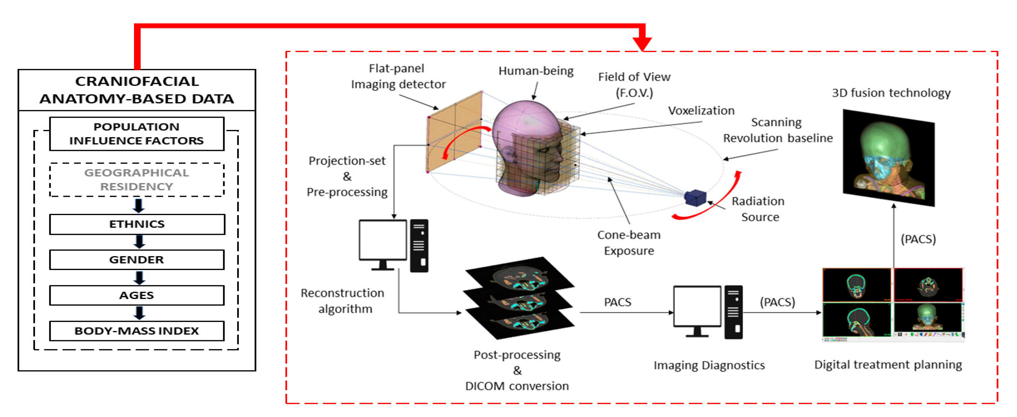
The schematic portfolio of our proposed method to enhance craniofacial skin tissue thickness segmentation is shown in Figure 1.

2.1. Materials and Equipment

As mentioned in [24], DCT100-0X0 CBCT configuration (Taiwan Care Tech Corporation (TCT), Kaohsiung, Taiwan), in Integrated Biomedical System Laboratory, Southern Taiwan University of Science and Technology, Tainan, Taiwan, was used in the mentioned SA2IR reconstruction. The reconstructed results were used as input for our proposed algorithm’s experiments. The experiments were implemented in the MATLAB environment (MATLAB 2017b, The Mathworks, Inc., Natick, MA, USA), processed by ASUS G531 (Intel^® Core™ i7-9750H CPU @2.60 GHz, 16 GB RAM, Nvidia GTX 1650 GPU, Taipei, Taiwan), supported by Nvidia CUDA toolkit 10.1 compilation. For our experimental works, a realistic digital patient head (RMDH) data of a young adult Caucasian male was used, provided by Aichert, A. et al., 2013 [28].

2.2. The Proposed Anatomic Moderators (PAM)

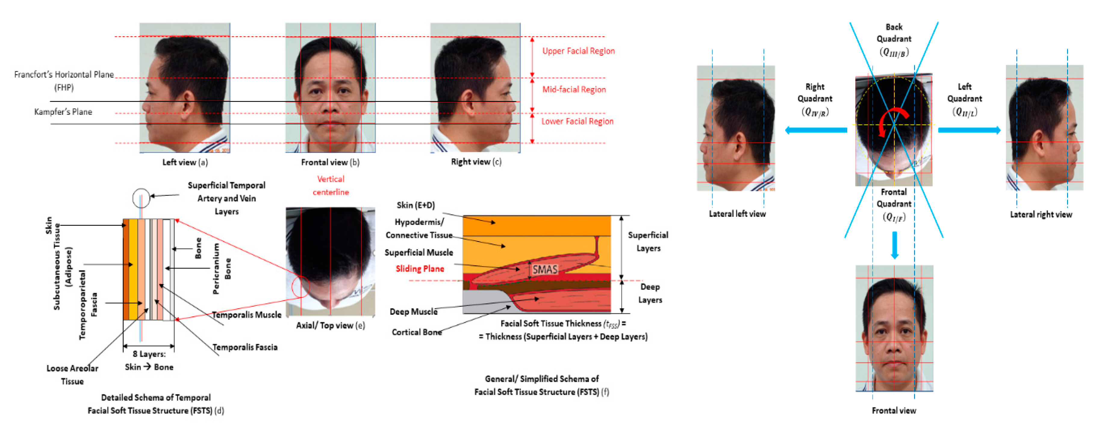
Corresponding to our selective anatomy analysis principle [24], facial soft tissue structure (FSTS) principal featuring was technically analyzed and morphologically decomposed into three facial regions and four quadrants (Figure 2). The anatomy layering is simply described in Figure 2. According to Ref. [12,13,14,29], the most effective and widely accepted craniofacial morphologic landmarking was proposed in De Greef, S. et al. [28], referred to

Table 1. Craniofacial soft tissue thickness landmarks [26,30].

No.	Landmarks	No.	Landmarks	No.	Landmarks
1	Supra-glabella 1	12/33	Supraorbital 2	23/44	Supra-glenoid 2
2	Glabella 2	13/34	Lateral glabella 2	24/45	Zygomatic arch 2
3	Nasion 2	14/35	Lateral nasal 2	25/46	Lateral orbit 2
4	End of nasion 2	15/36	Sub-orbital 2	26/47	Supra-M2 3
5	Mid-philtrum 3	16/37	Inferior malar 2	27/48	Mid masseter 3
6	Upper lip 3	17/38	Lateral nostril 3	28/49	Occlusal line 3
7	Lower lip 3	18/39	Nasolabial ridge 3	29/50	Sub-M2 3
8	Chin–lip fold 3	19/40	Supra-canine 3	30/51	Gonion 3
9	Mental eminence 3	20/41	Sub-canine 3	31/52	Mid-mandibula 3
10	Beneath chin 3	21/42	Mental tubercle anterior 3	-	-
11/32	Frontal eminence 1	22/43	Mid-lateral orbit 2	-	-

Notes: ¹ belong to the upper facial region (UFR), ² belong to the middle facial region (MFR) and ³ belong to the lower facial region (LFR).

. In the same study, a mass-populated sample of 510 females and 457 males of Caucasians was taken in craniofacial soft tissue thickness measurements that were used to update the contemporary Caucasian anthropometrics chart is updated and efficiently used in forensics and medical anatomy. Gender, ages, and body mass index (BMI) were systematically studied in correspondence. This has been indicated as a ground truth dataset for soft tissue and skin depth standardized inspections [12,29].

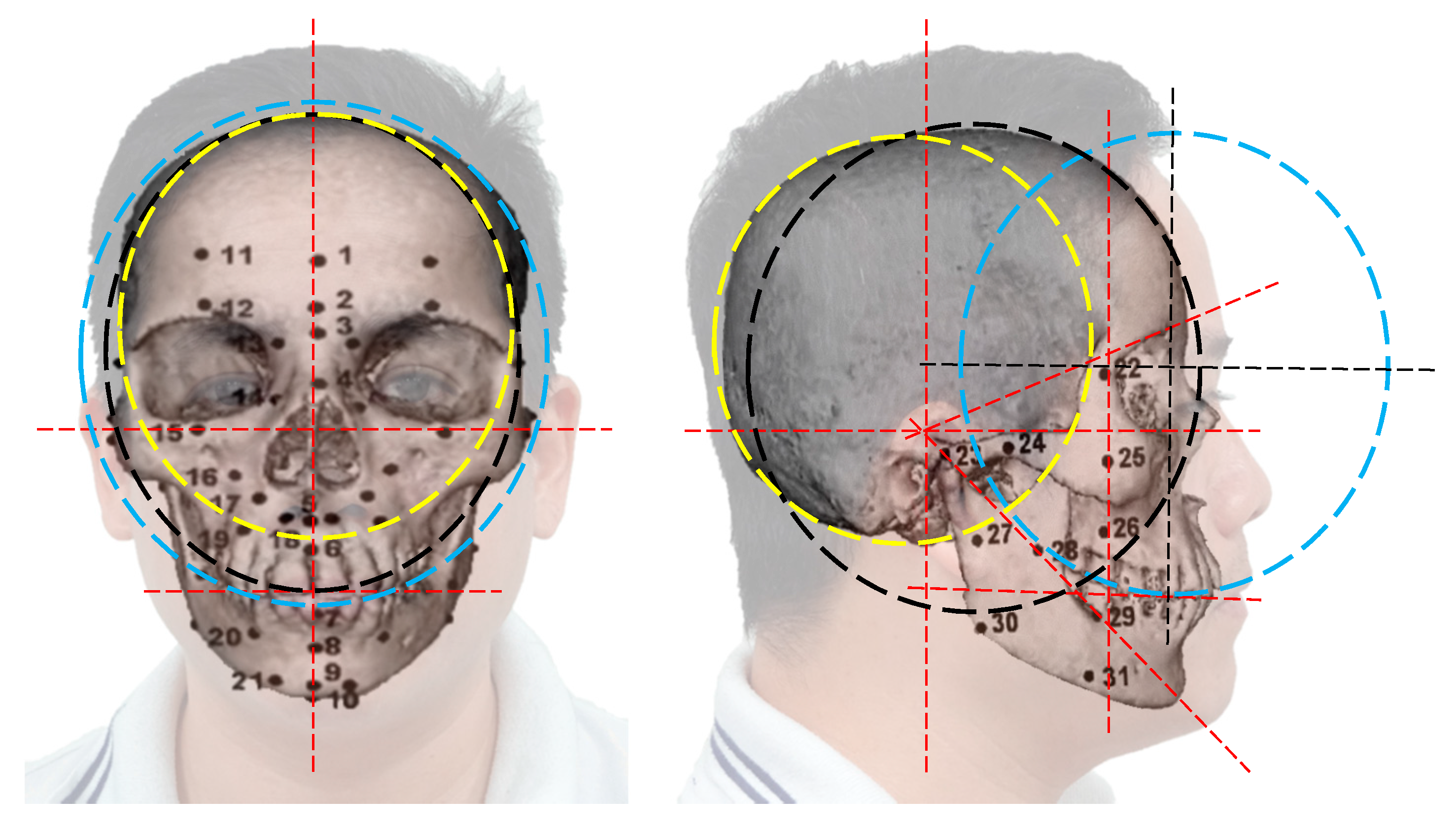
Due to the natural close-contoured and symmetric anatomy of a human head, 52 proposed landmarks (Figure 3 and Table 1) were re-grouped into the sufficient facial regions and quadrants, based on our anatomy analysis [26]. As per our proposal, the craniofacial database was used to generalize anatomy-specific moderators, named “the proposed anatomic moderators” (PAM). PAM was used as anatomic weights $w_{ij}^{PAM}$ for our proposed segmentation methods. Craniofacial symmetry is proven in [14,15,30]; thus the database was symmetrically built for left and right lateral quadrants. Based on our anatomic analysis, that was defined in three regions in height, as the upper region (UFR), middle region (MFR) and lower region (LFR) and in four quadrants radially, as the frontal quadrant ($Q_I$), left quadrant ($Q_{II}$), back quadrant ($Q_{III}$) and right quadrant ($Q_{IV}$).

Figure 3 and Table 1 describe 52 landmarks of facial soft tissue. The landmark numbers 1 to 10 are positioned on the coronal mid-line. The others are indicated symmetrically and bilaterally (left-sided and right-sided). For example, landmark 12/33 with #12 and #33 are left and right supraorbital, respectively. In Figure 3, the facial regional landmarking is defined into facial regions, such as (1) No. 1, 11 and 32 belong to UFR, (2) No. 2–4, 12–16, 22–25, 32–37 and 43–46 belong to MFR and (3) No. 5–10, 17–21, 26–31, 38–42 and 47–53 belong to LFR.

The verification conditions of PAM are listed as Caucasians validated, gender dimorphism neglected, monotonical-anatomy thresholded $\left\{T\right\}={{\displaystyle \cup }}_{i=1}^{N_T^{total}}\left\{T_i\right\}={{\displaystyle \cup }}_{i=1}^{N_T^{total}}{{\displaystyle \cup }}_{j=1}^{n_{i,k}}\left\{T_{i,j}\right\}$ and $N_T^{total}$ layering structure composed. In this, $\left\{T_{(·)}\right\}$ is the layered threshold of full anatomy $\left\{T\right\}$, tissue group $\left\{T_i\right\}$ and tissue sub-layer $\left\{T_{i,j}\right\}$. The number of tissue groups and number of tissue sub-layers is termed as $N_T^{total}$ and $n_{i,k}$, respectively.

Intrinsic to the attenuation nature of a given FSTS, the PAM is augmented to the biophysical exposure absorption behavior. Corresponding to Lambert–Beer’s law, $w_{ij}^{PAM}$ is calculated from attenuation coefficients (${\mu }_{i,j}^{PAM}$) and transmission traveling $t_{i,j}^{ODA}\left(x,y\right)$ of each specific tissue group or sub-layer, $\left\{T_i\right\}$ or $\left\{T_{i,j}\right\}$, as Equations (1) and (2).

$${t_{\Sigma }^{PAM}|}_{\left\{T\right\}}={\displaystyle \sum }_{i=1}^{N_T^{total}}{\displaystyle \sum }_{j=1}^{n_{i,k}}{t_{\mathrm{i},\mathrm{j}}^{PAM}|}_{\left\{T_i\right\}}$$

(1)

and

$$w_{i,j}^{PAM}=\frac{{\mu }_{\mathrm{i},\mathrm{j}}^{PAM}·t_{i,j}\left(x,y\right)}{{\overline{\mu }}_i^{PAM}·t_{\Sigma }^{PAM}}$$

(2)

where: ${\overline{\mu }}_i^{PAM}=\frac{1}{{\sum }_{i=1}^{N_T^{total}}{\sum }_{j=1}^{n_{i,k}}{t_{\mathrm{i},\mathrm{j}}^{PAM}|}_{\left\{T_i\right\}}}{\sum }_{i=1}^{N_T^{total}}{\sum }_{j=1}^{n_{i,k}}{t_{\mathrm{i},\mathrm{j}}^{PAM}.{\mu }_{\mathrm{i},\mathrm{j}}^{PAM}|}_{\left\{T_i\right\}}=-\frac{1}{t_{\left\{T_i\right\}}}·ln\left(\frac{I}{I_o}\right)$, while ${\mu }_{(·)}^{PAM}$ and $t_{(·)}^{PAM}$ 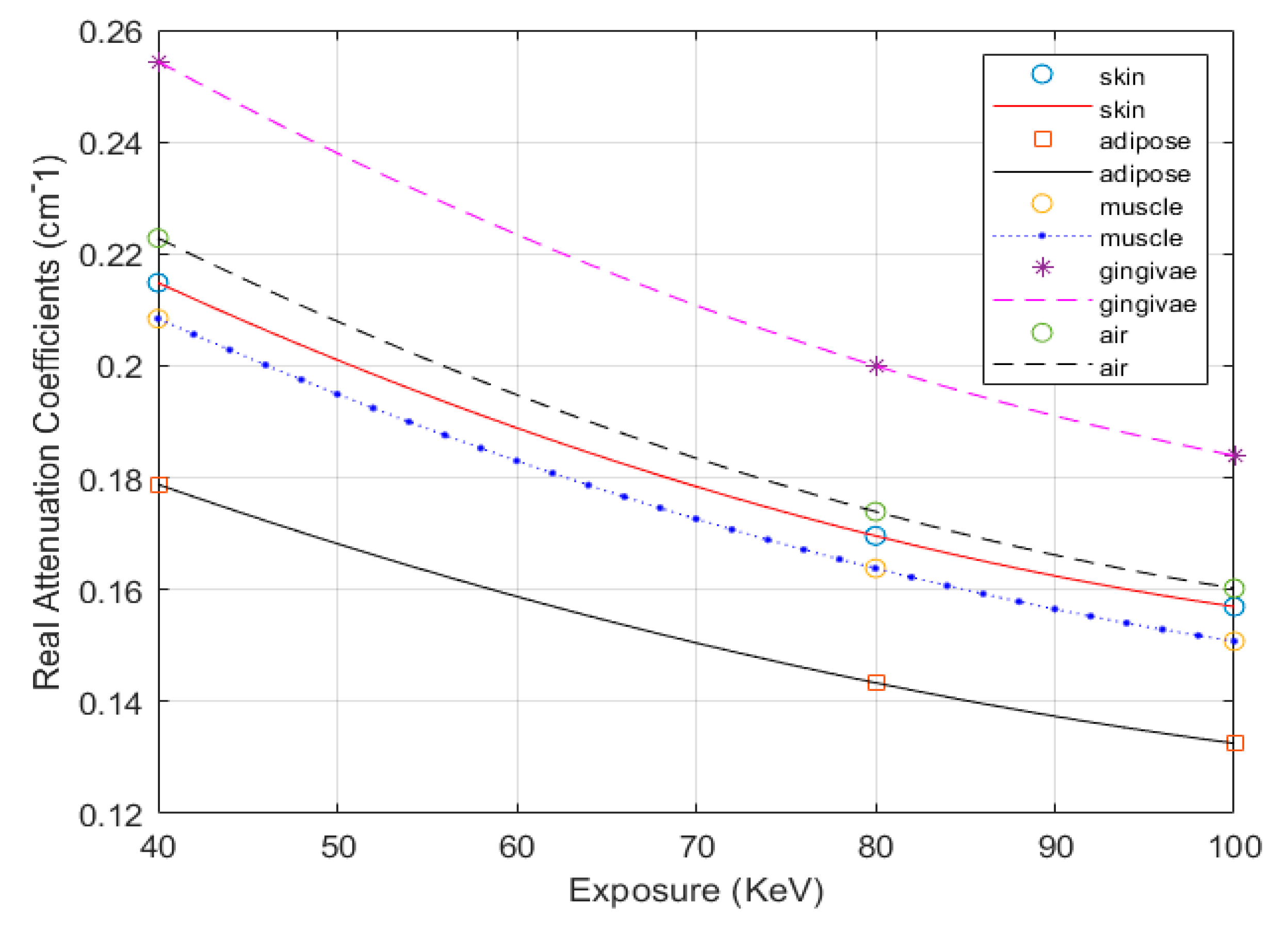are referred to as Tables 5.1, 5.2, B.1, and B.2 of ICRU Report 44 [18]. The new biophysical exposure attenuation coefficients of human soft tissue, in correspondence of PAM, are shown in

Table 2. Attenuation coefficients of human facial soft tissues.

Tissues	Specific Density ρ (kg/m3)	Mass Attenuation Coefficient µ/ρ (cm2/g)			Mass–Energy Absorption Coefficient µen/ρ (cm2/g)
Exposure Mode (keV)		40	80	100	40	80	100
Skin	1090.00	0.2620	0.1810	0.1690	0.0649	0.0254	0.0250
Adipose	916.00	0.2400	0.1800	0.1690	0.0448	0.0235	0.0243
Muscle	1050.00	0.2690	0.1820	0.1690	0.0705	0.0260	0.0254
Gingivae	1160.00	0.2972	0.2011	0.1867	0.0779	0.0287	0.0281
Air	1225.00	0.2490	0.1660	0.1540	0.0671	0.0240	0.0232

and Figure 4.

As the simplified layering structure (Figure 2), the craniofacial anatomy is decomposed into four tissue groups ($N_T^{total}=4$), as ambiance ($\left\{T_1\right\}$), soft tissues ($\left\{T_2\right\}$), hard tissues ($\left\{T_3\right\}$) and the supra-high substances (metallic artifacts) ($\left\{T_4\right\}$), respectively. Corresponding PAM moderators and their attenuation coefficients interpolation, the optimal thresholding, $\left\{T_i^{opt}\right\}=\left[\left\{T_{lb,i}^{opt}\right\},\left\{T_{ub,i}^{opt}\right\}\right]$, is computed in the grayscale of $\left[0,L_{GV,i}\right]$. The pixel-wise gray value of the adjacent $\left\{T_i^{opt}\right\}$ and $\left\{T_{i-1}^{opt}\right\}$ is computed as Equation (3).

$$g_i\left(x,y\right)-g_{i-1}\left(x,y\right)=\{\begin{array}{c}{\chi }_i^{ub},if{L}_{GV}\ge I\left(x,y\right)\ge \left\{T_{ub,i}^{opt}\right\}\\ {\chi }_i^{wt},if\left\{T_{ub,i}^{opt}\right\}>I\left(x,y\right)>\left\{T_{lb,i}^{opt}\right\}\\ {\chi }_i^{lb},if\left\{T_{lb,i}^{opt}\right\}\ge I\left(x,y\right)\ge 0\end{array}$$

(3)

With $g_{(·)}\left(x,y\right)$ is the chosen gray-value at pixel (x, y) of $\left\{T_{(·)}^{opt}\right\}$; $\left\{T_{lb,i}^{(·)}\right\}$ and $\left\{T_{ub,i}^{(·)}\right\}$ are the lower and upper bounds of $\left\{T_i^{(·)}\right\}$, respectively; $ub$, $lb$ and $wt$ stand for upper bound, lower bound and weighted; ${\chi }_{(,)}^{(·)}$ is the set threshold values of $\left\{T_{(·)}^{opt}\right\}$, while ${\chi }_{(·)}^{\left(ub\right)}\propto {\max }_{\left\{T_{(·)}\right\}}\left\{w_{i,j}^{PAM}.{\overline{t}}_{i,j}\left(x,y\right)\right\}$,${\chi }_{(·)}^{\left(lb\right)}\propto {\min }_{\left\{T_{(·)}\right\}}\left\{w_{i,j}^{PAM}.{\overline{t}}_{i,j}\left(x,y\right)\right\}$ and ${\chi }_{(·)}^{\left(wt\right)}\propto {\overline{w}}_{i,j}^{PAM}.{\overline{t}}_{i,j}\left(x,y\right)$; L_GV,i is the maximum gray-value of $\left\{T_i\right\}$.

The proposed anatomic analysis based craniofacial soft tissue thickness distribution of Caucasians is computed, shown in

Table 3. Proposed anatomic moderators (PAM)-based craniofacial soft tissue thickness.

Caucasians Aged (18–29)			The Proposed PAM-Based FSTS Thickness (in mm)
			Females						Males
BMI			<20		(20–25)		>25		<20		(20–25)		>25
Soft Tissue Thickness			μ	σ	μ	σ	μ	σ	μ	σ	μ	σ	μ	Σ
FSTS	UFR	QI/QIII	3.850	0.5500	4.000	0.600	4.500	0.650	3.850	0.430	4.100	0.595	4.900	0.905
		QII/QIV	3.800	0.500	3.900	0.600	4.500	0.600	3.800	0.470	4.100	0.640	5.000	0.960
	MFR	QI/QIII	6.999	1.287	7.354	1.356	8.155	1.405	6.319	1.123	6.717	1.287	7.941	1.606
		QII/QIV	7.700	1.750	8.250	1.850	9.500	1.900	6.950	2.080	7.743	2.032	9.550	2.460
	LFR	QI/QIII	11.35	1.894	11.502	1.945	12.246	2.156	11.465	1.918	11.834	2.063	12.816	2.080
		QII/QIV	16.367	2.567	17.000	2.700	18.800	3.100	15.867	2.427	16.879	2.912	19.867	3.357
SFSTS	UFR	QI/QIII	2.595	0.140	2.745	0.190	3.245	0.24	2.595	0.020	2.845	0.185	3.645	0.495
		QII/QIV	2.545	0.090	2.645	0.190	3.245	0.19	2.545	0.060	2.845	0.230	3.745	0.550
	MFR	QI/QIII	5.744	0.877	6.099	0.946	6.900	0.995	5.064	0.713	5.462	0.877	6.686	1.196
		QII/QIV	6.445	1.340	6.995	1.440	8.245	1.49	5.695	1.670	6.488	1.622	8.295	2.050
	LFR	QI/QIII	10.095	1.484	10.247	1.535	10.991	1.746	10.210	1.508	10.579	1.653	11.561	1.670
		QII/QIV	15.112	2.157	15.745	2.290	17.545	2.69	14.612	2.017	15.624	2.502	18.612	2.947

Notes: BMI is body-mass-index; FSTS and SFSTS are facial soft tissue structure and sub-skin facial soft tissue structure. UFR, MFR, and LFR are upper, middle, and low facial regions, respectively. Q_I, Q_II, Q_III, and Q_IV are the frontal, left, right and back quadrants, respectively.

.

2.3. Knapsack Problem in PAM-Based Craniofacial Soft Tissue or Skin Segmentation

Factually, the image segmentation task was a variation of the subset partitioning problem. Therefore, combinatorial optimization was used in our proposed method. The PAM-based craniofacial FSTS segmentation, as “PAM-based segmentation”, was modeled as a multi-choice knapsack problem (MCKP), constraints defined by PAM. According to [31], the general binary MCKP of PAM-base segmentation was as Equation (4).

$$\mathrm{maximize}{{\sum }_{i=1}^{N_T^{total}}{\sum }_{j=1}^{n_{i,k}}\left(w_{i,j}^{PAM}·t_{i,j}·x_{i,j}\right)|}_{\left\{T_i\right\}}$$

(4)

$$\begin{gathered} \mathrm{subject}\mathrm{to}:{\sum }_{i=1}^{N_T^{total}}{\sum }_{j=1}^{n_{i,k}}\left(w_{i,j}^{PAM}·t_{i,j}·x_{i,j}\right)-{\left\{T_{lb,i}^{opt}\right\}}_{ODA}\le {\left\{T_{ub,i}^{opt}\right\}}_{PAM}, \\ {\sum }_{i=1}^{N_T^{total}}{\sum }_{j=1}^{n_{i,k}}{t}_{i,j}=t_{\left\{T_i\right\}}, \end{gathered}$$

With $x_{i,j}\in \left\{0,1\right\}$, with $i=\left[1,4\right]$ and j = [1, n_k]. The specific attenuation of each {Ti} or {T_i,j}, is the subset–sum constraint. To solve, the Dantzig–Wolfe decomposition [32] and subset-sum partition ${\left(KSP\right)}_{\mathrm{i}}$ [33] are used, as the inverse problem ${\left(IKSP\right)}_{\mathrm{i}}$ of the known $n_{i,k}$ items, as Equations (5)–(7).

$${\left(KSP\right)}_{\mathrm{i}}\mathrm{minimize}min{z}_i\left({\beta }_i\right)={{{\displaystyle \sum }}_{i=1}^{N_T^{total}}{{\displaystyle \sum }}_{j=1}^{n_{i,k}}(w_{i,j}^{PAM}·t_{i,j}·x_{i,j})|}_{\left\{T_i\right\}}$$

(5)

$${\left(IKSP\right)}_{\mathrm{i}}\mathrm{minimize}{\beta }_i\left(z\right)$$

(6)

Reformed as:

$$\mathrm{maximize}z,\mathrm{subject}\mathrm{to}:{{{\displaystyle \sum }}_{j=1}^{n_{i,k}}{\beta }_i\left(z\right)|}_{\left\{T_i\right\}}\le \beta \mathrm{and}z\ge 0$$

(7)

Solve for the optimal value $z^{*}$ of (6):

$${{\displaystyle \sum }_{j=1}^{n_{i,k}}{\beta }_i\left(z\right)|}_{\left\{T_i\right\}}=\beta \Rightarrow z=z^{*}$$

(8)

$${{\displaystyle \sum }_{j=1}^{n_{i,k}}{\beta }_i\left(z\right)|}_{\left\{T_i\right\}}<\beta \Rightarrow z<z^{*}$$

(9)

$${{\displaystyle \sum }_{j=1}^{n_{i,k}}{\beta }_i\left(z\right)|}_{\left\{T_i\right\}}>\beta \Rightarrow z>z^{*}$$

(10)

As proposed Algorithm 1, the solution of Equation (4) is an iterative binary search algorithm, the decomposed per-each-iteration median efficiencies for each $\left\{T_i\right\}\in \left\{T\right\}$ is defined by $\overline{z}$. In the correspondence of ${\sum _{j=1}^{n_{i,k}}{\beta }_i\left(\overline{z}\right)|}_{\left\{T_i\right\}}$ value, the ${\left(IKSP\right)}_{\mathrm{i}}$ is solved by $\overline{z}$. The optimal $z^{*}$ is defined as the algorithm termination condition, shown in Equation (8). The initial item values of the concerned thresholds are eliminated, respectively, then replaced by 0 or 1, as mentioned in step 4 of Algorithm 1. The process is repeated while removing these fixed (decision) items from the problem. Corresponding to each threshold $\left\{T_i\right\}$, the profit sum of the fixed 1-valued items, named as $P_i$ and the $\left\{T_i\right\}$ is referred to as the updated set of remaining items. The threshold elimination is implemented as if the set of remaining items of $\left\{T_i\right\}$ is an individual (or $\left|T_i\right|=1$) and the ${\beta }_i\left(z\right)$ is simple linear functional.

Algorithm 1 Subset-sum partitioning to solve the PAM-based MCKP
Input:$\left\{T\right\}$, $\left\{T_i\right\}\in \left\{T\right\}$, $\beta$, ${\beta }_i$ and initial values of ${w_{i,j}^{PAM}|}_{\left\{T_i\right\}}$ Output: optimal solution for $z^{*}$ Begin
	Let $P_i:=0$ be the profit of the fixed 1-valued variables in each threshold $\left\{T_i\right\}$, $i=\left[1,N_T^{total}\right]$. The procedure is implemented as follow:
1:	For every remaining threshold of $\left\{T_i\right\}$, $i=\left[1,N_T^{total}\right]$, the median of the remained in the set of $\left\{\frac{p_{i,j}}{w_{i,j}}|j\in \left\{T_i\right\}={\cup }^{}\left({\left\{T_i\right\}}_L,{\left\{T_i\right\}}_G\right)\right\}$ is computed, as $r_i$. The subsets ${\left\{T_i\right\}}_L$ and ${\left\{T_i\right\}}_G$ are defined as followed: ${\left\{T_i\right\}}_L:=\left\{j\in \left\{T_i\right\}|\frac{p_{i,j}}{w_{i,j}}<r_i\right\}$ and ${\left\{T_i\right\}}_G:=\left\{j\in \left\{T_i\right\}|\frac{p_{i,j}}{w_{i,j}}\ge r_i\right\}$ And: $z_i:=\sum _{j\in G}\left(p_{i,j}+P_i\right)$ and $Z_i:=\left\{z_i,z_i,\dots ,z_i\right\}$, when $\left|Z_i\right|=\left|T_i\right|$.
2:	Compute $\overline{z}$, the median of the set $\left\{Z\right\}={{\cup }^{}}_{i=1}^{N_T^{total}}\left\{Z_i\right\}$.
3:	For $i=\left[1,N_T^{total}\right]$, solve the ${\left(IKSP\right)}_{\mathrm{i}}$ problem’s ${\beta }_i\left(\overline{z}\right)$. The stop condition is implemented, as if $\overline{z}$ is optimal, as Equation (8).
4:	For every threshold, variables elimination is executed as below:   $x_{i,k}=\{\begin{array}{c}1,if{\displaystyle \sum }{\beta }_i\left(z\right)\le \beta ,z<z^{*},and\frac{t_{i,j}}{w_{i,j}^{PAM}}\ge \frac{t_{i,k}}{w_{i,k}^{PAM}},t_{i,j},j\in \left\{T_i\right\}\\ 0,if{\displaystyle \sum }{\beta }_i\left(z\right)\le \beta ,z>z^{*},and\frac{t_{i,j}}{w_{i,j}^{PAM}}\le \frac{t_{i,k}}{w_{i,k}^{PAM}},t_{i,j},j\in \left\{T_i\right\}\end{array}$    1. Set $x_{ik}:=1,k\in {\left\{T_i\right\}}_G$, if the Equation (9) and $\overline{z}\ge z_i$ are achieved. 2. Set $x_{ik}:=1,k\in {\left\{T_i\right\}}_L$, if the Equation (10) and $\overline{z}\le z_i$ are achieved. Remove the fixed 1-valued item from the threshold, and accordingly update $P_i$.
5:	If n = 0, that means having no thresholds remained, then: Solve the current linear equation of ${\beta }_i\left(z\right)$ to find $z^{*}$. Else Return to step 1 of this algorithm.
End

2.4. The Proposed Segmentation Method for FSTS Narrow Low-Contrast Substances of FSTS

As mentioned, the shape-ness energy functional of deformable model differentiation, well-known as the “active contour” segmentation method, is widely used in medical image processing, due to its aggressive efficiency and accuracy [28]. With the previously known morphologic features, this algorithm is originated by McInertney, T. and Terzopoulos, D. (1996) [34], then modified by Karasev, P. et al., 2013 [35]. It has been developed in various approaches, such as faster computation regularization [36], edging featured for its geodesic model (GAC) [37], or using Chan–Vese’s energy functional (CVAC) [38]. To increase the sensitivity of CVAC, the integration of Mumford–Shah functional (MFS)—known as the MFS-CVAC method—was optimized by three subset-disjoint minimizers that regularize the bounded regions—inter versus outer sides ($I_{int}$ and $I_{ext}$) and perimeter of the contour $\Psi$. In advance, that smoothens each subset $\left\{T_{i,\left(j\right)}\right\}$ internally, while still maintaining the boundaries of the adjacent subsets, $\left\{T_{i,\left(j\right)}\right\}$ and $\left\{T_{i,\left(j-1\right)}\right\}$ [39]. However, due to undefined dimensionality, unknown morphology, and convex discontinuity of the given $I\left(x,y\right)$ and $\Psi$ morphology, the MFS-CVAC is easily ill-posed [40]. Because most of the real cases are piece-wise continuity, the weak form of MFS is preferred, without the region-bounded minimizer. That is called Blake-Zisserman functional ${ϵ}_{BZ}\left(I_{inter},I_{outer},\Psi \right)$ [41], as Equation (11). Hence, the craniofacial skin segmentation is the minimization of ${ϵ}_{BZ}\left(I_{inter},I_{outer},\Psi \right)$. Unlike the general soft tissue representation, the FSTS narrow low-contrast substance segmentation is still technically challenged in practice.

$$\begin{gathered} {ϵ}_{weak}\left(I_{int},I_{ext},\Psi \right)=\{{\lambda }_1{\int }_{\left\{T_2^{*}\right\}\backslash {\Psi }_{int}}||\nabla I_{int}||{}^{2}dxdy+{\lambda }_2{\int }_{\left\{T_2^{*}\right\}\backslash {\Psi }_{ext}}||\nabla I_{ext}||{}^{2}dxdy\} \\ +\xi ·length{|\Psi |}_{\{T_2^{*}\}} \end{gathered}$$

(11)

To solve this problem, we proposed the PAM-based segmentation algorithm for skin structure, described in Algorithm 2. In our method, the sagittal and coronal decompositions of each axial slice were priorly used to verify the real PAM with the pixel-wise subset composition. This created the MCKP for this application. Then, the optimal threshold of the concerned $\left\{T_{2,j}^{*}\right\}$ was solved as Algorithm 1. After updating, the cross-junctions of the concerned tissues were finally examined. The concerned tissue thickness was pixel-wise computed.

Algorithm 2 Proposed segmentation method
Input: Import the SA2IR reconstruction ${\mathsf{\Omega }}_{SA2RT}^3$, regional and quadrant sectioning and $n_{i,k}$ Output: cross-junction boundary and the thickness of facial combination skin Begin
1:	Threshold the FSTS out of the original images. The followed procedure is implemented on the FSTS-thresholded image only. Generate the sagittal and coronal decompositions of each axial slice.
2:	Compute the pixel-wise gray value of the corresponded projections per each facial region’s quadrant
3:	Implement the primary segmentation based on the preset number of concerned threshold values, as Equations (1)–(3).
4:	Calculate PAM, the optimum FSTS thickness equivalence as the known pixel-wise gray-value summation, calculated in step 2. Use subset-sum partitioning to solve the MCKP (Algorithm 1).
5:	Update the FSTS-thresholded image with the optimum $\left\{T_{2,j}^{*}\right\}$.
6:	Segment the final result, by minimizing Equation (11). Compute the PAM-based skin thickness pixel-wise.
End

2.5. Segmentation Efficiency Assessment Indices

In segmentation efficiency assessment of an $I\left(x,y\right)$ to the ground truth reference $I_o\left(x,y\right)$, Sørensen–Dice similarity coefficient (SDSC), as a Type I false measurement [42] and Jaccard similarity index (JSIM) [43] are used, as Equations (12) and (13). Theoretically, the more segmentation accuracy is defined, if and if only both SDSC and JSIM are closer to 1.

$$SDSC\left(I,I_o\right)=\frac{2.N\left\{I\left(x,y\right){{\displaystyle \cap }}^{}{I}_o\left(x,y\right)\right\}}{N\left\{I\left(x,y\right)\right\}+N\left\{I_o\left(x,y\right)\right\}},1\ge SDSC\left(I,I_o\right)\ge 0$$

(12)

and:

$$JSIM\left(I,I_o\right)=\frac{\left|I\left(x,y\right){{\displaystyle \cap }}^{}{I}_o\left(x,y\right)\right|}{\left|I\left(x,y\right){{\displaystyle \cup }}^{}{I}_o\left(x,y\right)\right|},1\ge JSIM\left(I,I_o\right)\ge 0$$

(13)

In Equation (12), $N\{·\}$ stands for the number of pixels in the enclosed set $\{·\}$, while the represents the results of different segment techniques applied to SA2IR reconstruction.

To evaluate the accuracy, the segmented soft tissue and skin thickness is compared to the contemporary Caucasian anthropometrics chart, mentioned above in Section 2.2. Herein, the correlation of different quadrants’ facial skin thicknesses ($t_{FST}^{Q_v}$) are defined, as $t_{FST}^{Q_{II}}=t_{FST}^{Q_{IV}}$ and $t_{FST}^{Q_{III}}=\left(1.2÷1.5\right)\times t_{FST}^{Q_I}$. The total facial skin is computed by the subtraction of FSTS and SFSTS thicknesses (Table 3).

3. Results and Discussion

The reconstruction of the realistic digital male head (RDMH) was implemented by the SA2IR algorithm, enriched by $k_{sampling}$ = 8 [26]. Using an exposure of 60-KeV and slicing with an interval of (0.5 ÷ 1.0) mm, the facial regions were defined along with the facial height. The upper facial region (UFR) was defined from the lowest point of the chin soft tissue to the nasal spine of the anterior maxillae (NSMA). The middle facial region (MFR) was defined from NSMA to the supra-glabella (anatomy landmark #2, Figure 3 and Table 1). The lower facial region (LFR) was defined from the supra-glabella to the highest point of cranial soft-tissue.

The three-dimensional construction was set as sagittal slice #180, coronal slice #180, and axial slice #100 (Figure 5a,b). The experimental segmented results were applied to the SA2IR reconstruction. The results of the proposed method were compared to the other active contour algorithms, including CVAC [38] and MFS-CVAC [38,39]. The segmented facial skin cross-junctions results are shown in

Table 4. Experimental results of Chan–Vese’s energy functional (CVAC), Mumford–Shah functional (MFS)-CVAC, and the proposed method on the axial slice #80.

	IQA Index	$\mathbf{CVAC}({\mathit{n}}_{2,\mathit{k}}\ge 3)$ [33]	$\mathbf{MFS}-\mathbf{CVAC}({\mathit{n}}_{2,\mathit{k}}\ge 3)$ [42]	The Proposed Method
Methods
SDSC		0	0	1
JSIM		0	0	1
Skin detection		X	X	√
Segmented result		Max. iterations = 300	Max. iterations = 3600	Max. iterations = 3000
Operation time (s)		8.970	77.540	45.8911 ($n_{2,k}$ = 4)

.

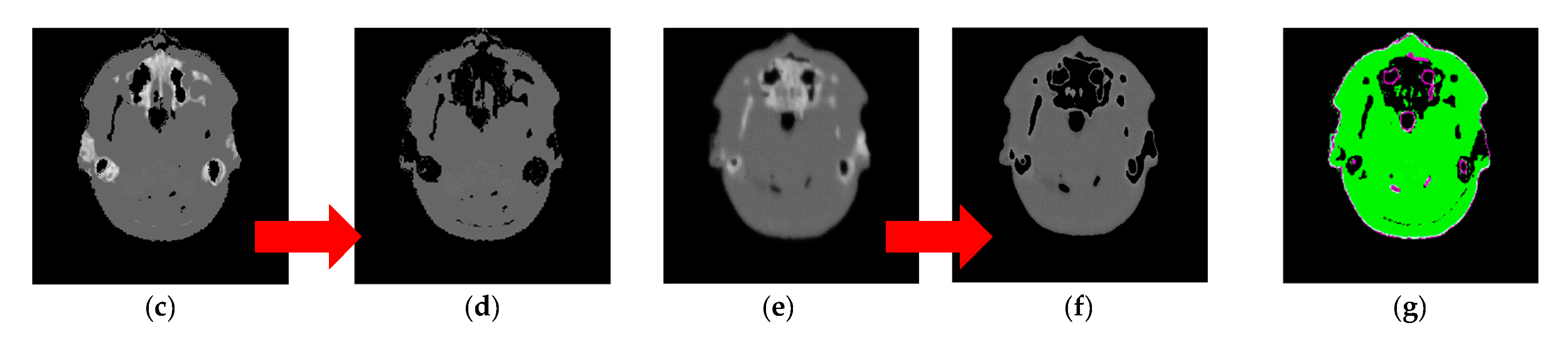
The original and SA2IR reconstructed images, herein called “inputs”, are shown in Figure 5a,b. The SA2IR reconstruction was gray-valued higher, blurred, and smoother than the original with the biased regions, shown at both the external-sided and internal-sided of contour due to GV abrasion (Figure 5c–f). That abrasion was proportional to the input sparsity and the enrichment coefficient of the SA2IR [22]. The differences between those are visually shown along with the transition gradient between $\left\{T_1\right\}$ and $\left\{T_{2,j}\right\}$ at facial and airway surfaces (the red circled in Figure 5b).

To eliminate noise and adjacent thresholds influences, the FSTS thresholded of those inputs was used for the accurate assessment. Quantitatively, the segmented thresholds the MFR axial slice #80 were (0.24763, 0.46987, 0.64822) (for SA2IR reconstruction) and (0.10583, 0.30593, 0.49014) (for original), respectively. Therefore, the FSTS threshold of those inputs was different, SA2IR 0.49014 (original input) versus 0.46987 (SA2IR’s input). The FSTS-threshold of those inputs was superimposed, shown in Figure 4g, with the purple FSTS outer contour. The matching accuracy of the initial segmentation of FSTS-thresholded inputs was 0.686727, in which the regional and boundary overlaps were in the approximations of 8.149% and 42.478%, respectively. The operation time for the input FSTS thresholding took 0.963 s, which was excluded from the experimental operation times, shown in Table 4.

In Table 4, over 1200 iterations, the local minima trap was detected while applying MFS-CVAC, circled red. That showed no facial skin structure detected, with the operation time of 76.001 s. Thus, their accuracy and specificity were valued “1”, but had zero values of SDSC and JSIM. In the same table, CVAC contrast showed no local minima trap and detected the skin tissue, but the average segmented thickness was thinner and out of the ground truth’s value. Better than the MFS-CVAC’s result, the CVAC’s operation was accomplished after 260 iterations (taken 8.221 s), with higher accuracy to the prior thresholded inputs, with the specificity of 1, the overall accuracy (0.69537) approximated to the raw inputs (0.68727). However, there was no significant differentiation in regional and boundary overlap (SDSC = 0, JSIM = 0). The segmented red-bounded contours showed the insufficient clustering, due to the “lost-data” of the black gap-offset between the purple contour and green region (Figure 4g). Conclusively, it was too difficult or impossible to define the skin structure, without prior known anatomic structure information.

In the proposed method’s results, the facial skin tissue was segmented, with different values of the number of anatomic interests $n_{2,k}$. In this, $n_{2,k}$ = 1 stands for no facial skin or no subset detection, $n_{2,k}$ = 2 for facial adipose skin, $n_{2,k}$ = 3 for facial skin and adipose and $n_{2,k}$ = 4 for facial skin, adipose, and muscles). As $n_{2,k}$ = 1, the result showed similar to the result of CVAC, due to step 6 of Algorithm 2. However, as $n_{2,k}=\left[3,4\right],$ there was no significant segmentation differentiation, when the maximum numbers of iterations were over 1250 iterations. As $n_{2,k}$ = 4, the experiment took 68.520 s to accomplish, with the segmented result shown in Table 4.

To evaluate the average skin thickness validation, with $\frac{t_{FST}^{Q_{III}}}{t_{FST}^{Q_I}}=1.5$, the average segmented thicknesses (in mm) of the proposed method were 3.1139 ± 0.8759 ($n_{2,k}$ = 2), 1.4220 ± 0.4000 ($n_{2,k}$ = 3) and 1.3181 ± 0.3708 ($n_{2,k}$ = 4). The ground-truth thickness of Caucasian males, aged (18–29) and having BMI < 20 is (1.25 ± 0.41) mm, taken by USM [30]. Pixel-wise, Algorithm 1 combinatorically optimized the solution, constrained by the anatomic and biophysical weighed PAM. Therefore, the proposed method’s results were higher adaptive to the ground-truth value. Exceptionally, in the case of $n_{2,k}$ = 2, the skin thickness was thicker than of the $n_{2,k}$ = 3 and $n_{2,k}$ = 4, due to the merging of skin and adipose.

Free of the pressurized deformation and gravitational effect as USM [12,26,29], our method was much more productive, due to a superlatively shorter operational time. In comparison to the ground-truth average skin thickness, the measurements’ of our method were skewed right, with the concern of $t_{FST}^{Q_{III}}$, while the ground-truth measurement was just implemented in the frontal and lateral quadrants ($Q_I$, $Q_{II}$ and $Q_{IV}$) only. However, it was not easy to define the skin thickness directly from echoing depth in USM in practice. Corresponding with the timing of the operation, it was significantly accelerated with our method. It took a couple of minutes for each slice segmentation, so that the skin thicknesses at 52 landmarks, axially defined on 10 working slices (1 UFR’s slice, 6 MFR’s slices, and 3 LFR’s slices), was found less than 20 min. Surprisingly, it took a couple of minutes for each landmark inspection in USM; thus, the total accomplishment time was up to 104 min. To the USM, the operation time was 5 times faster with the proposed method. Furthermore, the higher value of $n_{2,k}$ was chosen, the better result of skin tissue thickness was detected.

In practical terms, the proposed method causes no operator fatigue failure while doing mass- population data collection. To the conventional USM, that is much more inconvenient and dissatisfactory in action for both operators and volunteers/patients, who get involved in the measurements. Moreover, the measurements are much more difficult to operate and lesser accuracy on the slim-body (BMI < 20) and obese-body (BMI > 25) subjects. Similarly, that is problematic to the old aged subjects due to the FSTS plasticity and unstable placement at MFR’s and LFR’s landmarks. In our method, all of those issues are eliminated. For processing, our method just needs a field-of-view accommodated scan.

Combining the speed SA2IR algorithm [26], the proposed method significantly benefits the modern FSTS study, as shown above. Because the systematic anthropometric and/or anatomic statistical data quality or consistency were important keys of this method, the accuracy and efficiency were strongly dependent on the updating and refinement of the mass-population anatomic data. Therefore, in-depth collaboration between clinicians and technologists should be developed and improved along with time. However, it is difficult to do mass-population measurements at one time due to cost, workload, mass-population sampling challenges, and ethical constraints. To solve a part of those limitations, the shareable and online updated CBCT data management protocol was further studied and developed to improve the PAM database expansion not only on one ethnicity.

4. Conclusions

In conclusion, the proposed combination–optimization-based method was significantly efficient for facial skin structure segmentation and thickness measurements, due to ease of operation, computation speed, and no soft tissue deformation, in comparison to contact-probed methods. Using the previously known facial soft tissue anatomy and its biophysical properties, the skin thickness was identified much more easily and faster than with ultrasonic scanning methods. Furthermore, the proposed method also improved measurement consistency and productivity of the results due to the lack of dependence on human visual-ranking. This is in contrast with other digital imaging methods. The tool shows the potential to be an assistive tool for CBCT-driven studying lineage of anthropometrics, forensics, human archaeology, and some narrow medico-dental applications.

References

- Dao-Ngoc, L. The review of RP (Rapid Prototyping application in maxillofacial surgeries in Vietnam from 2010 to 2016: In the manufacturing engineer’s view. Cập nhật nha khoa—Tài liệu tham khảo và đào tạo liên tục 2017, 22, 121–142. [Google Scholar]
- Dao-Ngoc, L. A review of dental CAD/CAM technology: A story of past and present. Cập nhật nha khoa—Tài liệu tham khảo và đào tạo liên tục 2016, 21, 1–31. [Google Scholar]
- Kim, I.H.; Singer, S.R.; Mupparapu, M. Review of cone-beam computed tomography guidelines in North America. Quintessence Int. 2019, 50, 136–145. [Google Scholar] [PubMed]
- Hayashi, T.; Arai, Y.; Chikui, T.; Hayashi-Sakai, S.; Honda, K.; Indo, H.; Kawai, T.; Kobayashi, K.; Murakami, S.; Nagasawa, M.; et al. Committee on clinical practice guidelines Japanese society for, oral maxillofacial, radiology. Clinical guidelines for dental cone-beam computed tomography. Oral Radiol. 2018, 34, 89–104. [Google Scholar] [CrossRef]
- Bornstein, M.M.; Jorner, K.; Jacobs, R. Use of cone-beam computed tomography in implant dentistry: Current concepts, indications, and limitations for clinical practice and research. Periodontology 2017, 73, 51–72. [Google Scholar] [CrossRef]
- Jacobs, R.; Vranckx, M.; Vanderstuyft, T.; Quirynen, M.; Salmon, B. CBCT vs. other imaging modalities to assess peri-implant bone and diagnose complications: A systematic review. Eur. J. Oral Implant. 2018, 11, 77–92. [Google Scholar]
- Patel, S.; Brown, J.; Pimentel, T.; Kelly, R.D.; Abella, F.; Durack, C. Cone-beam computed tomography in Endodontics—A review of the literature. Int. Endod. J. 2019, 52, 1138–1152. [Google Scholar] [CrossRef] [Green Version]
- Woelber, J.P.; Fleiner, J.; Rau, J.; Ratka-Kruger, P.; Hannig, C. Accuracy and usefulness of CBCT in periodontology: A systematic review of the literature. Int. J. Periodontics Restor. Dent. 2018, 38, 289–297. [Google Scholar] [CrossRef] [Green Version]
- Qin, Z.; Zhang, X.; Li, Y.; Wang, P.; Li, J. One-stage treatment for maxillofacial asymmetry with orthognathic and contouring surgery using virtual surgical planning and 3D-printed surgical templates. J. Plast. Reconstr. Aesthet. Surg. 2019, 72, 97–106. [Google Scholar] [CrossRef]
- Fourie, Z.; Damstra, J.; Gerrits, P.O.; Ren, Y. Evaluation of anthropometric accuracy and reliability using different three-dimensional scanning systems. Forensic Sci. Int. 2011, 207, 127–134. [Google Scholar] [CrossRef]
- Bastir, M.; Rosas, A.; Lieberman, D.E.; O’Higgins, P. Middle cranial fossa anatomy and the origin of modern humans. Anat. Rec. 2008, 291, 130–140. [Google Scholar] [CrossRef] [PubMed]
- Stephan, C.N.; Meikle, B.; Freudenstein, N.; Taylor, R.; Claes, P. Facial soft tissue thicknesses in craniofacial identification: Data collection protocols and associated measurement errors. Forensic Sci. Int. 2019, 304, 109965. [Google Scholar] [CrossRef] [PubMed]
- De Donno, A.; Sablone, S.; Lauretti, C.; Mele, F.; Martini, A.; Introna, F.; Santoro, V. Facial approximation: Soft tissue thickness values for Caucasian males using cone-beam computer tomography. Leg. Med. 2019, 37, 49–53. [Google Scholar] [CrossRef] [PubMed]
- Hwang, H.S.; Park, M.-K.; Lee, W.J.; Cho, J.H.; Kim, B.K.; Wilkinson, C.M. Facial soft tissue thickness database for craniofacial reconstruction in Korean adults. J. Forensic Sci. 2019, 57, 1442–1447. [Google Scholar] [CrossRef]
- Berkhout, W.E.R. The ALARA-principle. Backgrounds and enforcement in dental practices. Ned. Tijdschr. Voor Tandheelkd. 2015, 122, 263–270. [Google Scholar] [CrossRef] [Green Version]
- Bushberg, J.T. Eleventh annual Warren K. Sinclair keynote address-science, radiation protection, and NCRP: Building on the past, looking to the future. Health Phys. 2015, 108, 115–123. [Google Scholar] [CrossRef]
- Ludlow, J.B.; Timothy, R.; Walker, C.; Hunter, R.; Benavides, E.; Samuelson, D.B. Effective dose of dental CBCT—A meta-analysis of published data and additional data for nine CBCT units. Dentomaxillofacial Radiol. 2015, 44. [Google Scholar] [CrossRef] [Green Version]
- McGuigan, M.B.; Duncan, H.F.; Horner, K. An analysis of effective dose optimization and its impact on image quality and diagnostic efficacy relating to dental cone beam computed tomography (CBCT). Swiss Dent. J. 2018, 128, 297–316. [Google Scholar]
- Fernandes, K.; Levin, T.L.; Miller, T.; Schoenfeld, A.H.; Amis, E.S., Jr. Evaluating an image gently and image wisely campaign in a multihospital health care system. J. Am. Coll. Radiol. 2016, 13, 1010–1017. [Google Scholar] [CrossRef]
- White, D.R.; Booz, J.; Griffith, R.V.; Spokas, J.J.; Wilson, I.J. ICRU report 44: Tissue substitutes in radiation dosimetry and measurement. J. Int. Comm. Radiat. Units Meas. 1989, 23, 198. [Google Scholar]
- Zhu, Z.G.; Wahid, K.; Babyn, P.; Cooper, D.; Pratt, I.; Carter, Y. Improved compressed sensing based algorithm for sparse-view CT image reconstruction. Comput. Math. Methods Med. 2013, 2013. [Google Scholar] [CrossRef] [PubMed] [Green Version]
- Zhang, C.; Zhang, T.; Zheng, J.; Li, Y.; You, J.; Guan, Y. A model of regularization parameter determination in low-dose X-ray CT reconstruction based on dictionary learning. Comput. Math. Methods Med. 2015, 2015, 790–831. [Google Scholar] [CrossRef] [PubMed] [Green Version]
- Matenine, D.; Goussard, Y.; Despres, P. GPU-accelerated regularized iterative reconstruction for few-view cone-beam CT. Med. Phys. 2015, 42, 1505–1517. [Google Scholar] [CrossRef] [PubMed]
- Chen, L.Y.; Liang, X.; Shen, C.Y.; Jiang, S.; Wang, J. Synthetic CT generation from CBCT images via deep learning. Med. Phys. 2020, 47, 1115–1125. [Google Scholar] [CrossRef] [PubMed]
- Kang, S.H.; Jeon, K.; Kim, H.J.; Seo, J.K.; Lee, S.H. Automatic three-dimensional cephalometric annotation system using three-dimensional convolutional neural networks: A developmental trial. Comput. Methods Biomech. Biomed. Eng. Imaging Vis. 2020, 8, 210–218. [Google Scholar] [CrossRef]
- Dao-Ngoc, L.; Du, Y.C. Generative noise reduction in dental cone-beam CT by a selective anatomy analytic iteration reconstruction algorithm. Electronics 2019, 8, 1381. [Google Scholar] [CrossRef] [Green Version]
- Stephan, C.N. Accuracies of facial soft tissue depth means for estimating ground-truth skin surfaces in forensic craniofacial identification. Int. J. Legal. Med. 2015, 129, 877–888. [Google Scholar] [CrossRef]
- He, J.; Kim, C.S.; Kuo, C.C.J. Interactive Segmentation Techniques: Algorithms and Performance Evaluation; SpringerBriefs in Signal Processing; Springer: Berlin/Heidelberg, Germany, 2014; ISBN 2096-4084. [Google Scholar]
- Aichert, A.; Manhart, M.T.; Navalpakkam, B.K.; Grimm, R.; Hutter, J.; Maier, A.; Hornegger, J.; Doerfler, A. A realistic digital phantom for perfusion C-arm CT based on MRI data. In Proceedings of the 2013 IEEE Nuclear Science Symposium and Medical Imaging Conference (2013 NSS/MIC), Seoul, Korea, 27 October–2 November 2013. [Google Scholar]
- De Greef, S.; Claes, P.; Vandermeulen, D.; Mollemans, W.; Suetens, P.; Willems, G. Large-scale in-vivo Caucasian facial soft tissue thickness database for craniofacial reconstruction. Forensic Sci. Int. 2006, 159, S126–S146. [Google Scholar] [CrossRef]
- Kellerer, H.; Pferschy, U.; Pisinger, D. Knapsack problems. In Handbook of Combinatorial Optimization; Springer: Berlin/Heidelberg, Germany, 2004; ISBN 3-540-40286-1. [Google Scholar]
- Pisinger, D. Budgeting with bounded multiple-choice constraints. Eur. J. Oper. Res. 2001, 129, 471–480. [Google Scholar] [CrossRef]
- Kuno, T.L.; Konno, H.; Zemel, E. A linear-time algorithm for solving continuous maximin knapsack problems. Oper. Res. Lett. 1991, 10, 23–26. [Google Scholar] [CrossRef]
- McInerney, T.; Terzopoulos, D. Deformable models in medical image analysis: A survey. Med. Image Anal. 1996, 1, 91–108. [Google Scholar] [CrossRef]
- Karasev, P.; Kolesov, I.; Fritscher, K.; Vela, P.; Mitchell, P.; Tannenbaum, A. Interactive medical image segmentation using PDE control of active contours. IEEE Trans. Med. Imaging 2013, 32, 2127–2139. [Google Scholar] [CrossRef] [PubMed]
- Goldenberg, R.; Kimmel, R.; Rivlin, E.; Rudzsky, M. Fast geodesic active contours. IEEE Trans. Image Process. 2001, 10, 1467–1475. [Google Scholar] [CrossRef]
- Casselles, V.; Kimmel, R.; Sapiro, G. Geodesic active contours. Int. J. Comput. Vis. 1997, 22, 61–79. [Google Scholar] [CrossRef]
- Chan, T.F.; Vese, L.A. Active contour without edges. IEEE Trans. Image Process. 2001, 10, 266–277. [Google Scholar] [CrossRef] [Green Version]
- Mumford, D.; Shah, J. Optimal approximations by piecewise smooth functions and associated variational problems. Commun. Pure Appl. Math. 1989, 42, 577–685. [Google Scholar] [CrossRef] [Green Version]
- Ramlau, R.; Ring, W. Regularization of ill-posed Mumford–Shah models with perimeter penalization. Inverse Probl. 2010, 26, 115001. [Google Scholar] [CrossRef]
- Blake, A.; Zisserman, A.; Bobrow, D.G.; Brady, M.; Davis, R.; Winston, P.H. Visual Reconstruction; MIT Press: Cambridge, MA, USA, 1987; ISSN 9780262255769. [Google Scholar]
- Wang, L.; Chang, Y.; Wang, H.; Wang, Z.Z.; Pu, J.T.; Yang, X.D. An active contour model based on local fitted images for image segmentation. Inf. Sci. 2017, 418, 61–73. [Google Scholar] [CrossRef] [Green Version]
- Shyu, K.K.; Pham, V.T.; Tran, T.T.; Lee, P.L. Unsupervised active contour driven by density distance and local fitting energy with applications to medical image segmentation. Mach. Vis. Appl. 2012, 23, 1159–1175. [Google Scholar] [CrossRef]
Figure 1.
Portfolio of the proposed method to enhance the segmentation of the low-contrast and narrow-banded substances in cone-beam computed tomography images.
Figure 2.
Anatomic facial soft tissue structure (FSTS), facial regions, and quadrants.
Figure 4.
The proposed PAM based attenuation coefficients.
Figure 5.
Slicing of the realistic digital male head (RDMH), showing original and selective anatomy analysis iterative reconstruction (SA2IR) on the axial slice #80. (a) Original data; (b) SA2IR reconstructed data; (c) original Image; (d) original only; (e) SA2IR Reconstruction; (f) SA2IR only; (g), FSTS superimposition of (d,f).