Material Identification Using a Microwave Sensor Array and Machine Learning


Department of Electrical and Computer Engineering, New York Institute of Technology, New York, NY 10023, USA
*
Author to whom correspondence should be addressed.
Electronics 2020, 9(2), 288; https://doi.org/10.3390/electronics9020288
Submission received: 16 January 2020
/
Revised: 1 February 2020
/
Accepted: 5 February 2020
/
Published: 8 February 2020
(This article belongs to the Special Issue Applications of Electromagnetic Waves)
Abstract
:In this paper, a novel methodology is proposed for material identification. It is based on the use of a microwave sensor array with the elements of the array resonating at various frequencies within a wide range and applying machine learning algorithms on the collected data. Unlike the previous microwave sensing systems which are mainly based on a single resonating sensor, the proposed methodology allows for material characterization over a wide frequency range which, in turn, improves the accuracy of the material identification procedure. The performance of the proposed methodology is tested via the use of easily available materials such as woods, cardboards, and plastics. However, the proposed methodology can be extended to other applications such as industrial liquid identification and composite material identification, among others.
1. Introduction
Microwave sensing has been utilized in a broad range of applications from noise measurement systems [1] and spatial displacement measurement [2] to single-cell viability detection [3] and material characterization [4,5].
One of the applications of microwave sensing is in material identification, which is a systematic approach to identify the particular grade of materials for reverse engineering, alteration, or repair of the existing assets or products and the use of substitute materials. In general, in microwave sensing and spectroscopy systems, the aim is to characterize the spectral behavior of the materials in a frequency range below 100 GHz. This can result in a low-cost integrated system for material identification and characterization. Conventionally, the sensing part of a microwave material characterization system is constructed using either a single resonator [6,7] or a transmission line (TL) [8].
In single-resonator sensors, the high quality factor (Q) of these devices renders the resonance frequency change due to the exposure to the material under test (MUT) measurable. However, this high sensitivity is only over a limited frequency band. If the tested MUTs have similar properties over the resonance band, they cannot be distinguished well. Here, we review some of the recent works in material identification using single-resonant-based sensors. In [9], a slot-loaded microstrip patch sensor antenna was proposed to enhance sensitivity in measuring the permittivity of planar materials. There, the antenna had two resonance frequencies, and the sensitivities of the |S11| responses to changes in the permittivities of the MUTs were studied. In [10], a microwave ring-resonator sensor was presented to evaluate the moisture content, or, more precisely, the water holding capacity, of broiler meat over a four-week period. There, the developed sensor showed significant changes in its resonance frequency and return loss due to the reduction in water holding capacity in the studied duration. In [11], a metamaterial-based microwave sensor with a complementary split ring resonator (CSRR) was implemented for dielectric characterization of liquids. Liquid samples placed inside glass capillary tubes modify the resonant frequency and Q-factor of the CSRR sensor. Thereby, a relation between the sensor resonant frequency, Q-factor, and complex permittivity of the liquid samples was established. In [12], a method was presented to estimate the complex permittivity of liquids based on an embedded microstrip line with a CSRR etched in the ground plane, beneath the conductor strip. A liquid container surrounding the CSRR was added to the structure in order to load the sensing element, i.e., CSRR, with the liquid under test. The complex permittivity of the liquid was inferred from the frequency response of the structure, particularly from the change in the response at resonant frequency.
On the other hand, transmission-line-based sensors are suitable for broadband sensing with reduced sensitivity. According to the above-mentioned discussions, tackling the tradeoff between the sensitivity and bandwidth to achieve broadband material identification is challenging. Thus, in this paper, a material identification system is proposed based on a microwave sensor array with the elements of the array resonating at different frequencies, covering a wide band. This allows us to benefit from the excellent sensitivity of the high-Q resonators while, similar to the TL approach, collecting information over a wide bandwidth. A machine learning algorithm is then developed to identify different materials based on the data collected by the microwave sensor array. We use an automatic framework that consists of a multiclass support vector machine (SVM) classification based on a decision tree approach [13].
The performance of the proposed material identification system is validated via testing of three groups of materials made of cardboard, wood, and plastic. The results show satisfactory performance of the system in distinguishing these three groups of materials. The advantages of the proposed material identification system include its compactness, low cost, and low error rate, and its contactless, reusable, easy-to-fabricate, and easy-to-work operation.
2. Microwave Sensor Array
In this section, we review the design of a microwave sensor array first proposed in [14] for water quality testing. The array is composed of five resonating elements, as shown in Figure 1. These resonating elements are based on a microstrip transmission line loaded with CSRRs designed at different frequencies within the range of 1 GHz to 10 GHz. The use of planar CSRR sensors offers several advantages such as low cost, portability, noninvasiveness, and flexibility of sample preparation. This is why they have been widely used for sensing applications (see, e.g., [15,16,17,18]).
The sensor array in Figure 1 allows for measuring changes in dielectric properties over a wide frequency range from 1 GHz to 10 GHz, specifically at five frequencies around 1 GHz, 3 GHz, 5 GHz, 7 GHz, and 9 GHz. Changes in the dielectric properties can then be monitored through measuring the resonance frequency shifts for the resonator array.
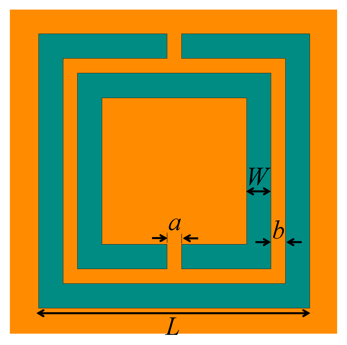
The design of the sensor array was implemented in Altair FEKO software [19]. It is high-frequency electromagnetic simulation software based on the method of moments (MoM). The sensor array was designed on a Rogers RO4350 substrate with dielectric properties of εr = 3.66 and tan δ = 0.0031. The width Ws, length Ls, and thickness of the substrate are 20 mm, 56 mm, and 0.75 mm, respectively. The microstrip line was designed to have a characteristic impedance of 50 Ω. This corresponds to the width of strip line being Wm = 1.68 mm. This strip line was placed at the center of the front surface of the substrate. On the back side of the substrate, the five CSRRs were etched out of the ground plane. Figure 1 shows the front and back sides of the designed sensor array. The CSRRs, as shown in Figure 1b, were named Sensor 1 to Sensor 5 from left to right and correspond to resonance frequencies of 1.36 GHz, 3.09 GHz, 5 GHz, 6.82 GHz, and 8.91 GHz. Figure 2 shows the main design parameters for each CSRR structure, including the length of the outer ring L, width of the rings W, the track width between adjacent rings b, and the width of narrow lines a. As a rule of thumb, a larger value of L corresponds to a lower resonance frequency, and as W increases, the resonance frequency decreases. Table 1 and Table 2 show the optimal design parameters and center-to-center distances for the sensor array, respectively.
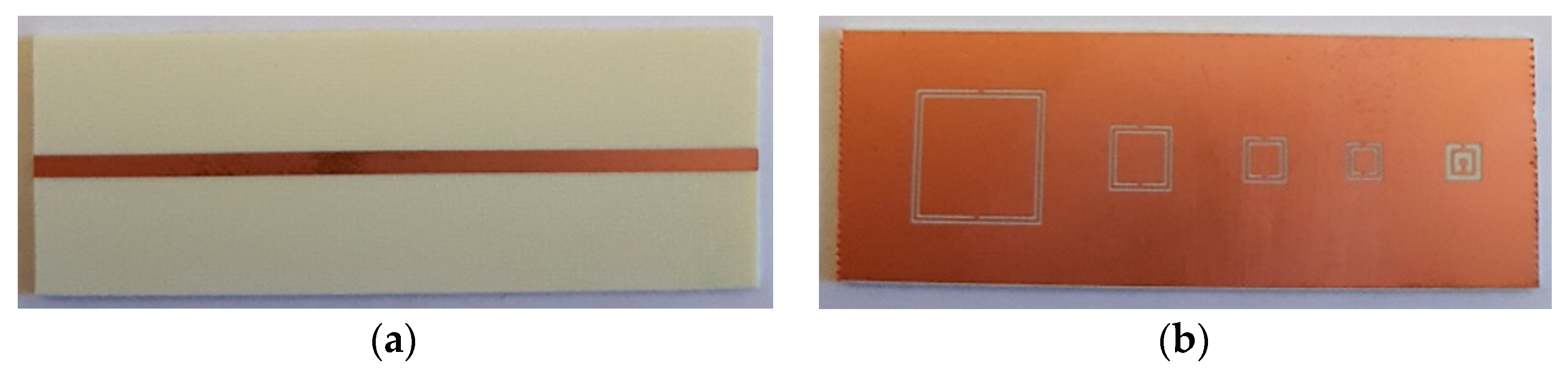
The sensor array was fabricated using printed circuit board technology (PCB) as shown in Figure 3. Sub-Miniature A (SMA) connectors were soldered on both ends of the microstrip transmission line, and the whole device was installed on a wooden stand piece to ensure a mechanically stable platform for conducting the measurements.
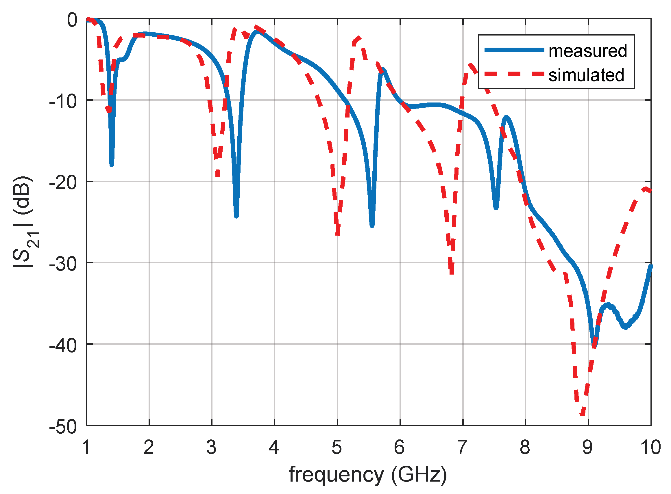
In order to record the response of the sensor array to the materials, the variation of the transmission S-parameter |S21| versus frequency was measured without any MUT using an E5063A vector network analyzer (VNA) from Keysight Technologies. Figure 4 shows a comparison of the simulated and measured |S21| for the sensor array. A reasonable match can be observed between the simulated and measured results. The mismatches may be due to the fabrication tolerances and soldering. Please note that the difference between the measured |S21| in [14] and that here is due to the fact that the measured |S21| in [14] is for a sensor array with a plexiglass container placed on the back side of it for measuring water samples, while the measured |S21| reported here in Figure 4 is for a bare sensor array. Furthermore, in Figure 4, an additional resonance is observed for the measured |S21| at around 9.6 GHz. It is worth noting that this extra resonance is not utilized in our material characterization, described later, since it is very close to the other resonance frequency at 9.1 GHz for which the data will be used in our processing. In fact, the data from this additional resonance at 9.6 GHz would be very similar to those from 9.1 GHz due to approximately similar material properties at these two close frequencies. This justifies the use of data only at 9.1 GHz.
3. Machine Learning Algorithm
The use of an array of resonator sensors allow us to process the collected data using proper machine learning algorithms. As shown later, such a system provides significantly more accurate results compared to the use of a single resonator sensor. In the following, we describe the three MUT categories and the machine learning approach utilized to distinguish them.
3.1. Three Groups of MUTs
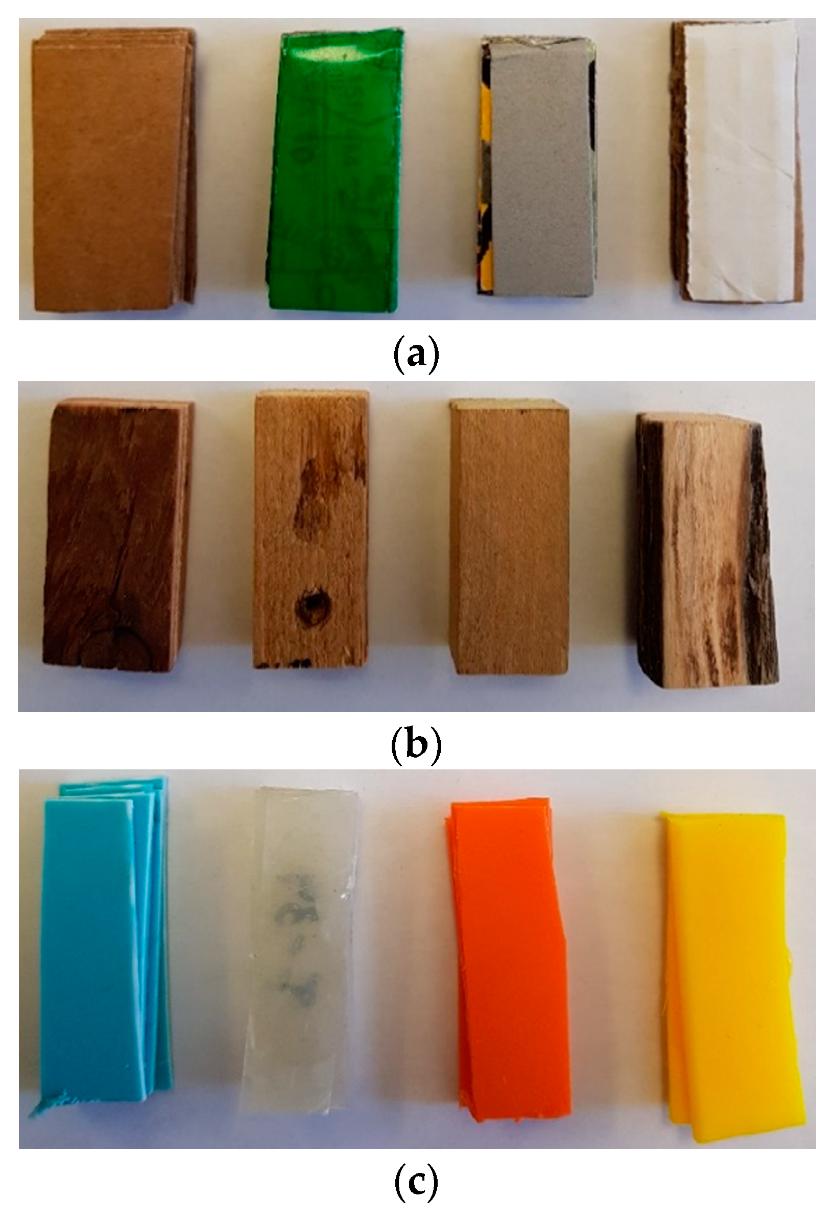
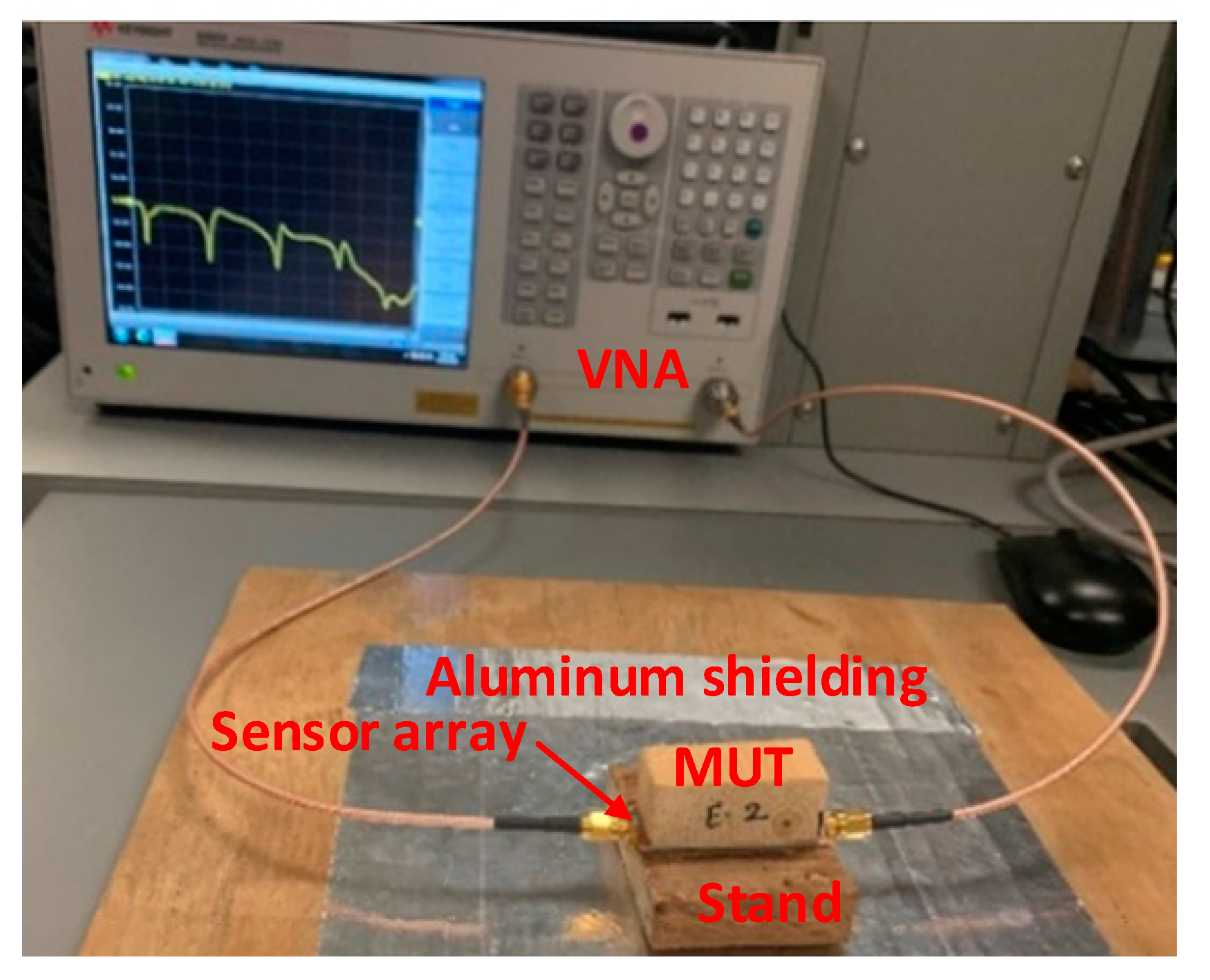
To validate the performance of the proposed material identification system, three groups of MUTs were measured with the microwave sensor array. These three MUT groups were (1) 50 cardboard samples, (2) 50 wood samples, and (3) 50 plastic samples. Figure 5 shows pictures of a few samples from each group. Figure 6 shows the measurement setup in which the MUTs were placed on the back side of the sensor array (the side containing the CSRR elements) and |S21| versus frequency was measured using an E5063A ENA from Keysight Technologies.
3.2. Feature Selection
To evaluate the performance of the microwave sensor array in distinguishing the three groups of MUTs described above, we used the shifts in the five resonant frequencies in the |S21| response due to exposure to the MUT as our features. We then applied different combinations of the five features to the classifier, from selecting only one feature to using all five features. Therefore, the total number of combinations that were used for classification was 31 (see Table 3).
3.3. Outlier Detection and Removal
In order to detect the data samples that were away from other samples in each class, i.e., outliers, we used the k-Nearest Neighbor (KNN) outlier detection algorithm available in the PyOD toolbox (Python Toolbox for Scalable Outlier Detection) [20]. It uses the math behind the KNN classification algorithm. Indeed, for any data point, the distance to its k-many nearest neighbors could be viewed as the outlying score. We used the median distance to these k neighbors to detect outliers, where k = 5 was considered in this study.
3.4. Decision-Tree-Based Support Vector Machine
In this study, we use a decision-tree-based support vector machine (DSVM) approach for classifying the three categories of cardboard, wood, and plastic samples. The rationale behind this is that combining decision tree architecture with binary SVMs allows us to benefit from the advantages of the efficient computation of decision trees and the high classification accuracy of SVMs. The chosen kernel function was a Gaussian radial basis function using Scikit-learn, the machine learning library in Python [21].
4. Results
In this section, we evaluate the performance of the proposed approach in distinguishing the three groups of MUTs discussed in the previous section. First, in order to detect possible outliers, KNN outlier detection was applied to data samples in each group. We found four outliers in cardboard data samples, three outliers in wood data samples, and three outliers in plastic data samples that were then removed from the dataset. Therefore, the total number of data samples was reduced to 140, including 46 cardboard samples, 47 wood samples, and 47 plastic samples.
The median ± median absolute deviation (MAD) of each resonant frequency shift for the three MUTs, along with the corresponding p values using the Wilcoxon rank sum test over each pair of MUTs, is shown in Table 4. From Table 4, the median resonant frequency shift is significantly different in cardboard samples in comparison to wood samples for Sensors 1 to 4 and plastic samples for Sensors 2 to 5. Furthermore, the median resonant frequency shift is significantly higher in wood samples in comparison to plastic samples for all five sensors, which suggests the possibility to distinguish these three MUTs with a machine learning algorithm.
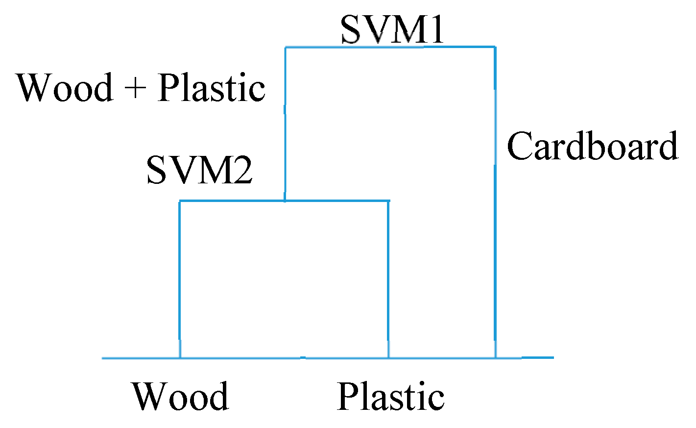
The hierarchical cluster analysis step for the DSVM machine learning approach is shown in Figure 7. Since the cardboard samples are filled with air gaps, their electrical properties are highly different from those of wood and plastic samples. Therefore, at the top of the tree (i.e., the root node), the first binary classifier (SVM1) is trained to classify the cardboard class (a terminal node) as a negative class and the remaining merged two classes (wood + plastic) as a positive class. Then, the second binary classifier in the tree (SVM2) is trained to classify the elements of plastic as a negative class and the elements of wood as a positive class.
Leave-one-out (LOO) and stratified k-fold class validation (SKF) procedures [22] were used to evaluate the classification performance. The LOO procedure is an iterative process where, in each iteration, all the features associated with one particular data sample are taken as a test dataset and are omitted from the training set. The iterations repeat until all data samples have been taken as a test dataset once. The SKF procedure is also an iterative process. In this procedure, first the data samples are split into k-many groups (folds) where in each fold the same proportion of data samples is considered for each class. Then, at each iteration, one fold is taken as a test dataset and is omitted from the training set. The iteration is repeated until all folds have been taken as a test dataset once. In this study, the value of k was 5. The performance of the DSVM approach was then compared with that of some widely used machine learning approaches: decision tree (DT), random forest (RF), k-nearest neighbors (KNN), Gaussian naive Bayes (GNB), and multilayer Perceptron (MLP), where 10 trees was considered for the RF approach, 5 neighbors was considered for the KNN approach, and 1 hidden layer with 5 neurons was considered for the MLP approach to get the best corresponding classification performance.
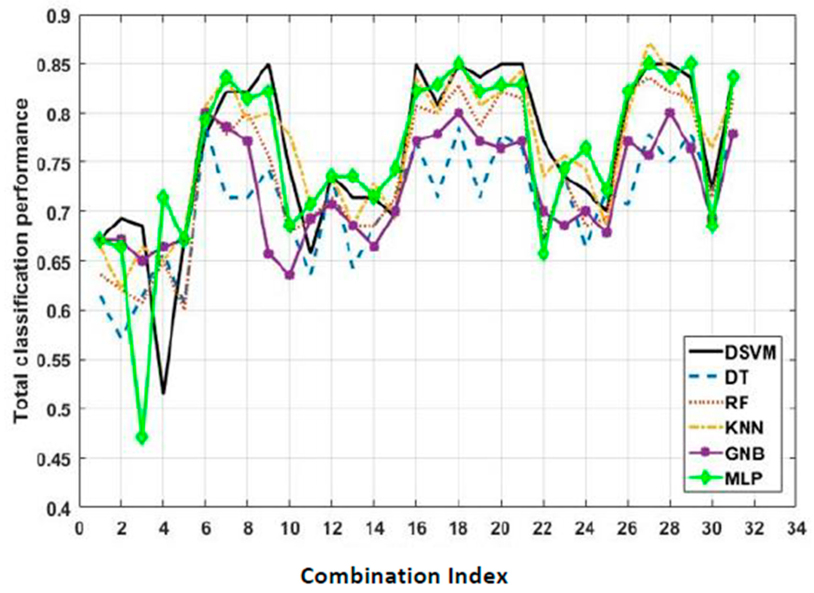
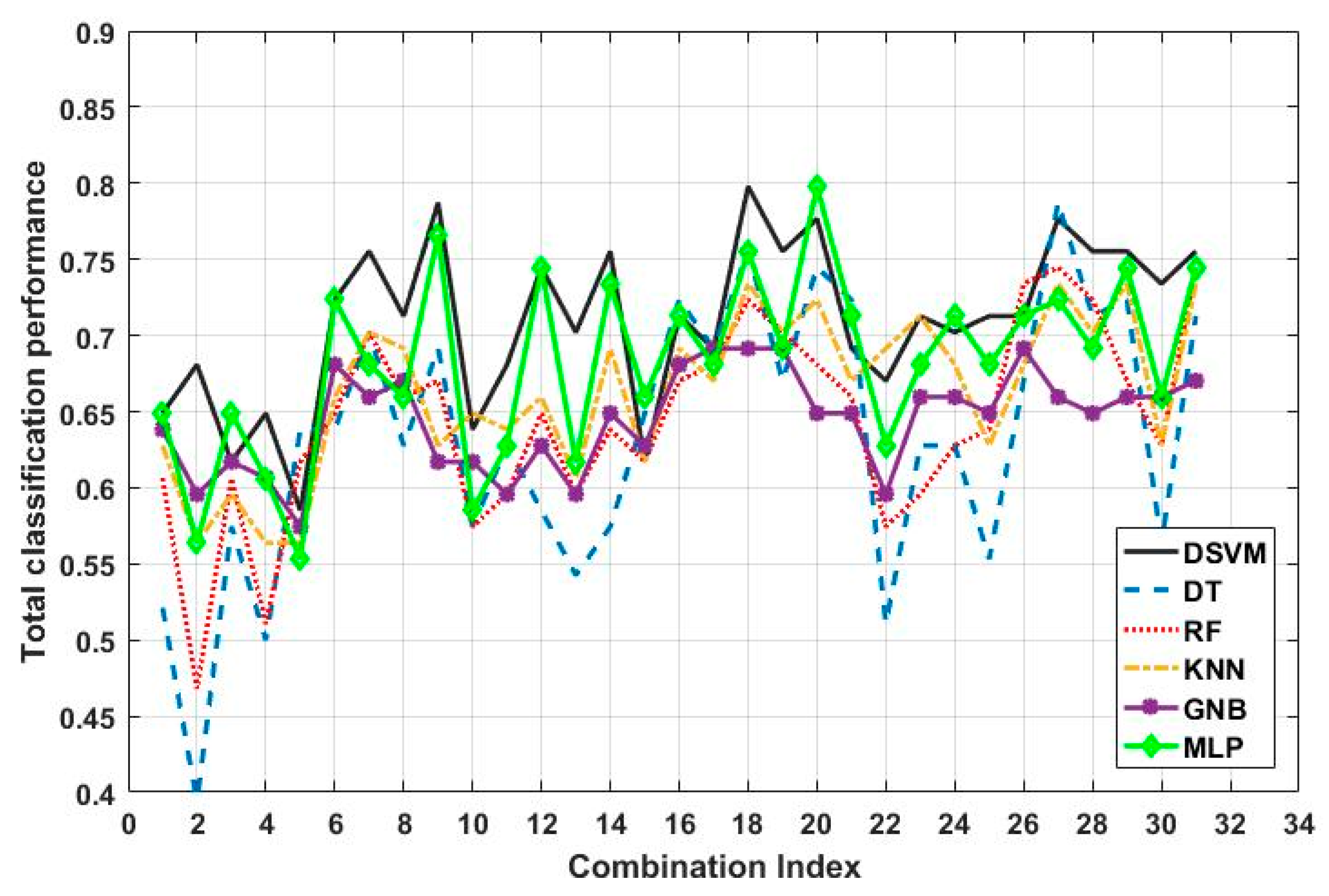
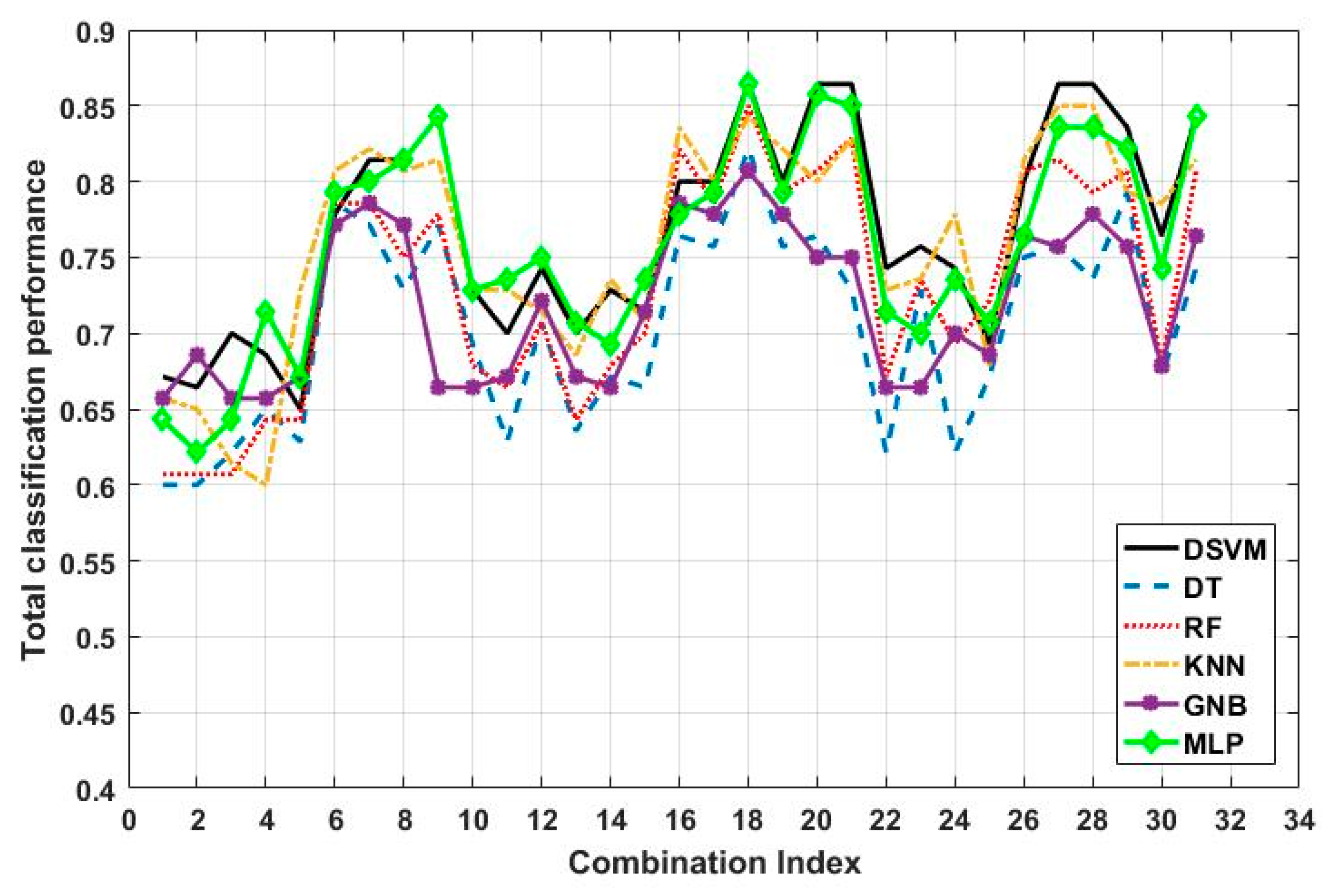
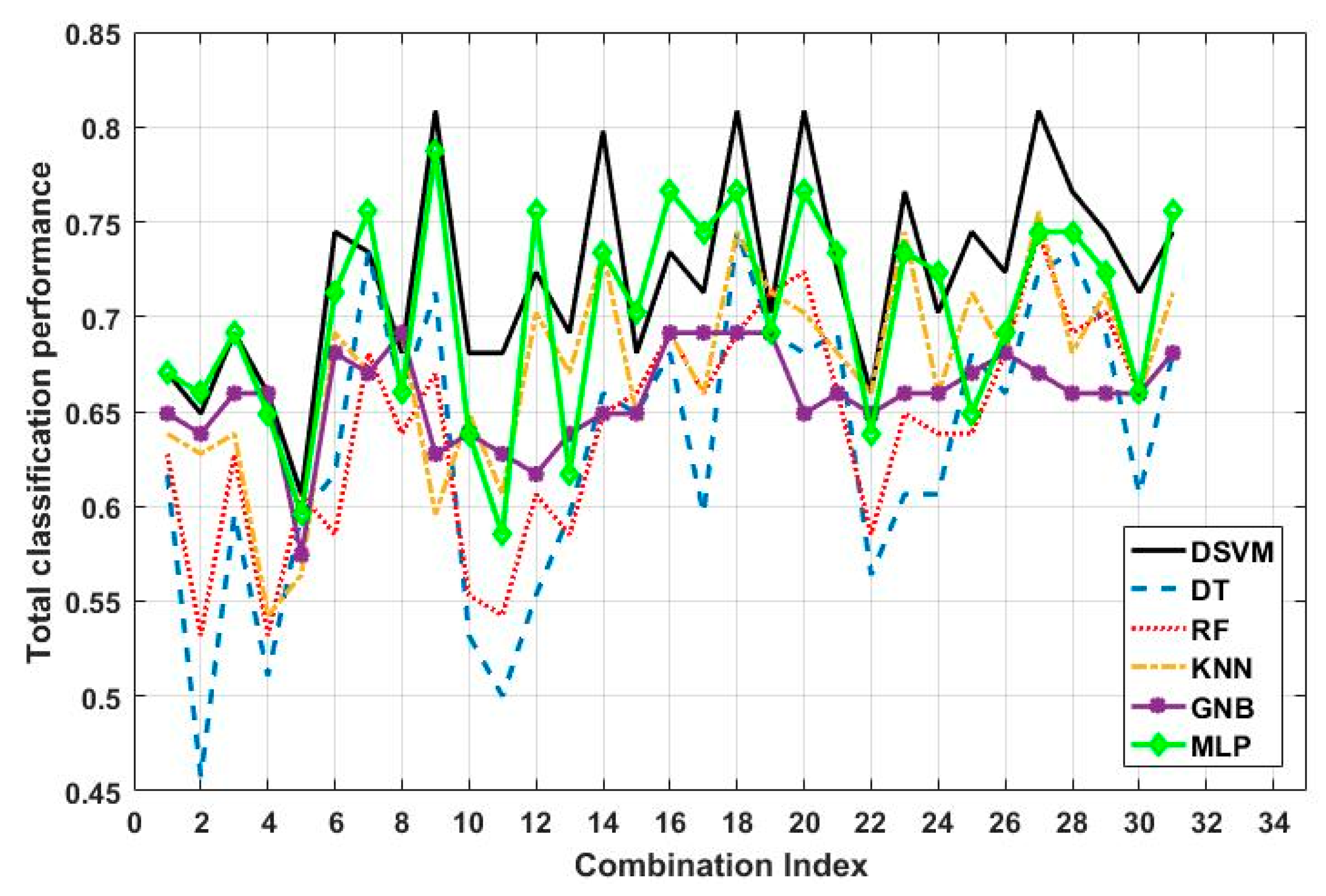
To demonstrate the classification accuracy for each of the 31 combinations of the 5 features, Figure 8, Figure 9, Figure 10 and Figure 11 depict the total classification performance versus feature combination index when classifying cardboard versus the rest and wood versus plastic using LOO and SKF cross-validation approaches. The relationship between the combination index and the combination of sensors is shown in Table 3, where the first index belongs to the case where the resonance frequency shift in the first sensor is used as the feature, the second index belongs to the case where the resonance frequency shift in the second sensor is used as the feature, and so on. From these figures, the classification performance was less than 70% when using the resonant frequency shift of each single sensor for all approaches using both LOO and SKF cross-validation. However, using LOO cross-validation for classifying cardboard versus the rest, the performance was higher than 80% for 3 to 14 out of the 31 combinations that involve at least two sensors, where the lowest number belonged to the GNB approach and the highest number belonged to the DSVM, MLP, and KNN approaches (Figure 8). Furthermore, using SKF cross-validation, the performance was higher than 80% for 1 to 14 out of the 31 combinations, where the lowest number belonged to the GNB and DT approaches and the highest number belonged to the DSVM and KNN approaches (Figure 10). Using LOO cross-validation, the classification performance for classifying wood and plastic was higher than 75% for 0 to 10 out of the 31 combinations that involve at least two sensors, where the lowest number belonged to the GNB, KNN, and RF approaches and the highest belonged to the DSVM approach (Figure 9). Furthermore, using SKF cross-validation, the performance was higher than 75% for 0 to 7 out of the 31 combinations, where the lowest number belonged to the GNB, DT, and RF approaches and the highest number belonged to the DSVM and MLP approaches (Figure 11).
The highest classification performance for classifying cardboard versus the rest using the LOO cross-validation approach belonged to KNN (87%) for feature combination index 27, where the selected features were the resonance frequency shifts in Sensors 1, 2, 3, and 5 (see Table 3), followed by the DSVM approach (85%) for feature combination indices 16, 18, 20, 21, 27, and 28 and by the MLP (85%) approach for feature combination indices 18, 27, and 29. However, the best classification performance for classifying cardboard versus the rest using SKF and also for classifying wood from plastic using both LOO and SKF cross-validation belonged to the DSVM approach at multiple feature combinations with common feature combination index 18 (the resonance frequency shifts in Sensors 1, 2, and 5). This confirms that the DSVM approach has the highest and most consistent overall performance in terms of the selected features.
Table 5 and Table 6 show the corresponding confusion matrix along with the sensitivity, specificity, and total accuracy of the DSVM approach for feature combination index 18 using the LOO cross-validation approach. From Table 5, the highest classification performance was 85% for classifying cardboard versus the rest. Furthermore, from Table 6, wood and plastic were classified with a highest classification performance of 79.8%. The corresponding classification performance using SKF cross-validation is shown in Table 7 and Table 8, where the highest classification performance was 86.4% for classifying cardboard versus the rest and 81.9% for classifying wood and plastic. These results demonstrate that the proposed procedure can classify both cardboard from the rest and wood from plastic with high accuracy.
5. Conclusions
This study for the first time proposed a material identification methodology using a wideband microwave sensor array and machine learning. The sensor array is composed of five planar resonating elements (sensors) designed at different frequencies within the range of 1 GHz to 10 GHz and has several advantages such as low cost, portability, noninvasiveness, reusability, and flexibility of sample preparation. A machine learning approach was then applied to the data collected from these five sensors to classify three MUTs: cardboard, wood, and plastic. The utilized features were the resonant frequency shifts in the five sensors due to exposure to MUTs. In this study, we utilized a DSVM classifier to first classify cardboard from the rest (wood + plastic) and then classify wood and plastic. We examined all 31 combinations of the 5 measured frequency shifts. We then compared the performance of the DSVM with that of widely used machine learning approaches: DT, RF, KNN, GNB, and MLP. The results showed that the DSVM approach had the highest and most consistent classification performance with both LOO and SKF cross-validation when using the resonant frequency shifts in Sensors 1, 2, and 5 as selected features. This demonstrated that the proposed approach could classify the three MUTs with high accuracy. By collecting more samples, the proposed approach can be used as an accurate automatic technique for identifying materials that are used in buildings, bridges, and structures such as swimming pool panels, racing car bodies, bathtubs, storage tanks, etc.
Author Contributions
Conceptualization, R.K.A.; methodology, R.K.A. and M.R.; software, L.H., M.R., and K.Z.; validation, L.H., M.R., K.Z., D.T., and T.P.; formal analysis, L.H. and M.R.; investigation, all the authors; resources, R.K.A. and M.R.; data curation, L.H. and M.R.; writing—original draft preparation, R.K.A., M.R., and L.H.; writing—review and editing, R.K.A. and M.R.; visualization, all of the authors; supervision, R.K.A. and M.R.; project administration, R.K.A. and M.R.; funding acquisition, R.K.A. All authors have read and agreed to the published version of the manuscript.
Funding
This research was funded by a New York Institute of Technology’s Institutional Support for Research and Creativity (ISRC) Grant.
Conflicts of Interest
The authors declare no conflict of interest.
References
- Ivanov, E.N.; Tobar, M.E.; Woode, R.A. Microwave interferometry: Application to precision measurements and noise reduction techniques. IEEE Trans. Ultrason. Ferroelect. Freq. Control 1998, 45, 1526–1536. [Google Scholar] [CrossRef] [PubMed]
- Kim, S.; Nguyen, C. A displacement measurement technique using millimeter-wave interferometry. IEEE Trans. Microw. Theory Techn. 2003, 51, 1724–1728. [Google Scholar]
- Yang, Y.; Zhang, H.; Zhu, J.; Wang, G.; Tzeng, T.; Xuan, X.; Huang, K.; Wang, P. Distinguishing the viability of a single yeast cell with an ultra-sensitive radio frequency sensor. Lab Chip 2010, 10, 553–555. [Google Scholar] [CrossRef] [PubMed]
- Schueler, M.; Mandel, C.; Puentes, M.; Jakoby, R. Metamaterial inspired microwave sensors. IEEE Microw. Mag. 2012, 13, 57–68. [Google Scholar] [CrossRef]
- Jilani, M.T.; Rehman, M.Z.; Khan, A.M.; Khan, M.T.; Ali, S.M. A brief review of measuring techniques for characterization of dielectric materials. Int. J. Inf. Elect. Eng. 2012, 1, 1–5. [Google Scholar]
- Cherpak, N.T.; Barannik, A.A.; Prokopenko, Y.V.; Smirnova, T.A.; Filipov, Y.F. A New Technique of Dielectric Characterization of Liquids; Springer: Amsterdam, The Netherlands, 2005. [Google Scholar]
- Bernard, P.A.; Gautray, J.M. Measurement of dielectric constant using a microstrip ring resonator. IEEE Trans. Microw. Theory Techn. 1991, 39, 592–595. [Google Scholar] [CrossRef]
- Cataldo, A.; Benedetto, E.D.; Cannazza, G. Quantitative and Qualitative Characterization of Liquid Materials; Springer: Berlin, Germany, 2011; pp. 51–83. [Google Scholar]
- Yeo, J.; Lee, J. Slot-loaded microstrip patch sensor antenna for high-sensitivity permittivity characterization. Electronics 2019, 8, 502. [Google Scholar] [CrossRef] [Green Version]
- Jilnai, M.; Wen, W.; Cheong, L.; Rehman, M.Z. A microwave ring-resonator sensor for non-invasive assessment of meat aging. Sensors 2016, 16, 52. [Google Scholar] [CrossRef] [PubMed]
- Chuma, E.L.; Iano, Y.; Fontgalland, G.; Roger, L.L.B. Microwave sensor for liquid dielectric characterization based on metamaterial complementary split ring resonator. IEEE Sens. J. 2018, 18, 9978–9983. [Google Scholar] [CrossRef]
- Su, L.; Mata-Contreras, J.; Vélez, P.; Martín, F. Estimation of the complex permittivity of liquids by means of complementary split ring resonator (CSRR) loaded transmission lines. In Proceedings of the IEEE MTT-S International Microwave Workshop Series on Advanced Materials and Processes for RF and THz Applications (IMWS-AMP), Pavia, Italy, 20–22 September 2017. [Google Scholar]
- Lajnef, T.; Chaibi, S.; Ruby, P.; Aguera, P.E.; Eichenlaub, J.B.; Samet, M.; Kachouri, A.; Jerbi, K. Learning machines and sleeping brains: Automatic sleep stage classification using decision-tree multi-class support vector machines. J. Neurosci. Methods 2015, 250, 94–105. [Google Scholar] [CrossRef] [PubMed]
- Zhang, K.; Amineh, R.K.; Dong, Z.; Nadler, D. Microwave sensing of water quality. IEEE Access 2019, 7, 69481–69493. [Google Scholar] [CrossRef]
- Boybay, M.S.; Ramahi, O.M. Material characterization using complementary splitring resonators. IEEE Trans. Instrum. Meas. 2012, 61, 3039–3046. [Google Scholar] [CrossRef]
- Lee, C.-S.; Yang, C.-L. Thickness and permittivity measurement in multi-layered dielectric structures using complementary split-ring resonators. IEEE Sens. J. 2014, 14, 695–700. [Google Scholar] [CrossRef]
- Lee, C.-S.; Yang, C.-L. Complementary split-ring resonators for measuring dielectric constants and loss tangents. IEEE Microw. Wirel. Compon. Lett. 2014, 24, 563–565. [Google Scholar] [CrossRef]
- Ansari, M.A.H.; Jha, A.K.; Akhtar, M.J. Design and application of the CSRR-based planar sensor for noninvasive measurement of complex permittivity. IEEE Sens. J. 2015, 15, 7181–7189. [Google Scholar] [CrossRef]
- Altair FEKO Software. Available online: https://altairhyperworks.com/product/FEKO (accessed on 8 February 2020).
- Zhao, Y.; Nasrullah, Z.; Li, Z. PyOD: A Python Toolbox for Scalable Outlier Detection. J. Mach. Learn. Res. 2019, 20, 1–7. [Google Scholar]
- Pedregosa, F.; Varoquaux, G.; Gramfort, A.; Michel, V.; Thirion, B.; Grisel, O.; Blondel, M.; Prettenhofer, P.; Weiss, R.; Dubourg, V.; et al. Scikit-learn: Machine Learning in Python. J. Mach. Learn. Res. 2011, 12, 2825–2830. [Google Scholar]
- Hastie, T.; Tibshirani, R.; Friedman, J. The Elements of Statistical Learning: Data Mining, Inference, and Prediction, 2nd ed.; Springer: Berlin, Germany, 2009. [Google Scholar]
Figure 1.
Microwave sensor array (a) front surface and (b) back surface with Sensor 1 to Sensor 5, shown from left to right, corresponding to resonance frequencies of 1.36 GHz, 3.09 GHz, 5 GHz, 6.82 GHz, and 8.91 GHz, respectively.
Figure 1.
Microwave sensor array (a) front surface and (b) back surface with Sensor 1 to Sensor 5, shown from left to right, corresponding to resonance frequencies of 1.36 GHz, 3.09 GHz, 5 GHz, 6.82 GHz, and 8.91 GHz, respectively.

Figure 2.
Parametric model of each complementary split ring resonator (CSRR).

Figure 3.
Fabricated sensor array (a) front surface and (b) back surface.

Figure 4.
Simulated and measured |S21| for the sensor array.

Figure 5.
Pictures of a few samples measured for each category: (a) cardboard samples, (b) wood samples, and (c) plastic samples.
Figure 5.
Pictures of a few samples measured for each category: (a) cardboard samples, (b) wood samples, and (c) plastic samples.

Figure 6.
Measurement of |S21| for the sensor array using a vector network analyzer (an E5063A ENA from Keysight Technologies).
Figure 6.
Measurement of |S21| for the sensor array using a vector network analyzer (an E5063A ENA from Keysight Technologies).

Figure 7.
A decision-tree-based support vector machine (SVM) generated for the three classes of cardboard, wood, and plastic.
Figure 7.
A decision-tree-based support vector machine (SVM) generated for the three classes of cardboard, wood, and plastic.

Figure 8.
Total classification accuracy versus combination index for classifying cardboard from the rest for different classification approaches using LOO cross-validation.
Figure 8.
Total classification accuracy versus combination index for classifying cardboard from the rest for different classification approaches using LOO cross-validation.

Figure 9.
Total classification accuracy versus combination index for classifying wood and plastic for different classification approaches using LOO cross-validation.
Figure 9.
Total classification accuracy versus combination index for classifying wood and plastic for different classification approaches using LOO cross-validation.

Figure 10.
Total classification accuracy versus combination index for classifying cardboard from the rest for different classification approaches using SKF cross-validation.
Figure 10.
Total classification accuracy versus combination index for classifying cardboard from the rest for different classification approaches using SKF cross-validation.

Figure 11.
Total classification accuracy versus combination index for classifying wood and plastic for different classification approaches using SKF cross-validation.
Figure 11.
Total classification accuracy versus combination index for classifying wood and plastic for different classification approaches using SKF cross-validation.


Table 1.
Dimensions of the designed CSRRs.
| fr (GHz) | W (mm) | L (mm) | a (mm) | b (mm) | |
|---|---|---|---|---|---|
| Sensor 1 | 1.36 | 0.27 | 10.5 | 0.16 | 0.16 |
| Sensor 2 | 3.09 | 0.27 | 5.15 | 0.16 | 0.16 |
| Sensor 3 | 5 | 0.27 | 3.65 | 0.16 | 0.16 |
| Sensor 4 | 6.82 | 0.27 | 3 | 0.16 | 0.16 |
| Sensor 5 | 8.91 | 0.54 | 3 | 0.16 | 0.16 |
Table 2.
Distance between CSRRs as shown in Figure 1b.
Table 2.
Distance between CSRRs as shown in Figure 1b.
| X1 (mm) | X2 (mm) | X3 (mm) | X4 (mm) | X5 (mm) | X6 (mm) |
|---|---|---|---|---|---|
| 11 | 13 | 10 | 8 | 8 | 6 |
Table 3.
Relationships between combination indices and combinations of sensors.
| Combination Index | Combinations of Sensors | Combination Index | Combinations of Sensors |
|---|---|---|---|
| 1 | 1 | 17 | 1, 2, 4 |
| 2 | 2 | 18 | 1, 2, 5 |
| 3 | 3 | 19 | 1, 3, 4 |
| 4 | 4 | 20 | 1, 3, 5 |
| 5 | 5 | 21 | 1, 4, 5 |
| 6 | 1, 2 | 22 | 2, 3, 4 |
| 7 | 1, 3 | 23 | 2, 3, 5 |
| 8 | 1, 4 | 24 | 2, 4, 5 |
| 9 | 1, 5 | 25 | 3, 4, 5 |
| 10 | 2, 3 | 26 | 1, 2, 3, 4 |
| 11 | 2, 4 | 27 | 1, 2, 3, 5 |
| 12 | 2, 5 | 28 | 1, 2, 4, 5 |
| 13 | 3, 4 | 29 | 1, 3, 4, 5 |
| 14 | 3, 5 | 30 | 2, 3, 4, 5 |
| 15 | 4, 5 | 31 | 1, 2, 3, 4, 5 |
| 16 | 1, 2, 3 |
Table 4.
Median (± median absolute deviation (MAD)) values of resonant frequency shift across all MUT samples, along with Wilcoxon rank sum test p values comparing each resonant frequency shift for each pair of MUTs.
Table 4.
Median (± median absolute deviation (MAD)) values of resonant frequency shift across all MUT samples, along with Wilcoxon rank sum test p values comparing each resonant frequency shift for each pair of MUTs.
| Resonant Frequency Shift (MHz) | Cardboard | Wood | Plastic | p Values (Cardboard, Wood) | p Values (Cardboard, Plastic) | p Values (Wood, Plastic) |
|---|---|---|---|---|---|---|
| Δf1 | 81.00 ± 11.70 | 94.50 ± 18.00 | 73.80 ± 16.20 | 0.0012 | 0.18 | 3.28 × 10⁻⁴ |
| Δf2 | 150.75 ± 31.95 | 122.40 ± 31.50 | 84.60 ± 41.40 | 0.0141 | 5.13 × 10⁻⁴ | 0.032 |
| Δf3 | 225.00 ± 57.15 | 162.00 ± 63.90 | 92.70 ± 62.10 | 0.0026 | 7.10 × 10⁻⁵ | 0.026 |
| Δf4 | 241.20 ± 75.15 | 147.60 ± 86.40 | 52.20 ± 58.50 | 6 × 10⁻⁴ | 1.34 × 10⁻⁴ | 0.027 |
| Δf5 | 331.65 ± 163.80 | 308.70 ± 206.10 | 96.30 ± 145.80 | 0.78 | 9.14 × 10⁻⁴ | 0.004 |
Table 5.
DSVM classification performance for classifying cardboard vs. the rest using LOO cross-validation.
Table 5.
DSVM classification performance for classifying cardboard vs. the rest using LOO cross-validation.
| Class | Wood + Plastic | Cardboard | Sensitivity | Specificity | Total Accuracy |
|---|---|---|---|---|---|
| Wood + Plastic | 84 | 10 | 89.4% | 76.1% | 85% |
| Cardboard | 11 | 35 |
Table 6.
DSVM classification performance for classifying wood vs. plastic using LOO cross-validation.
Table 6.
DSVM classification performance for classifying wood vs. plastic using LOO cross-validation.
| Class | Wood | Plastic | Sensitivity | Specificity | Total Accuracy |
|---|---|---|---|---|---|
| Wood | 39 | 8 | 83.0% | 76.6% | 79.8% |
| Plastic | 11 | 36 |
Table 7.
DSVM classification performance for classifying cardboard vs. the rest using SKF cross-validation.
Table 7.
DSVM classification performance for classifying cardboard vs. the rest using SKF cross-validation.
| Class | Wood + Plastic | Cardboard | Sensitivity | Specificity | Total Accuracy |
|---|---|---|---|---|---|
| Wood + Plastic | 86 | 8 | 91.5% | 76.1% | 86.4% |
| Cardboard | 11 | 35 |
Table 8.
DSVM classification performance for classifying wood vs. plastic using SKF cross-validation.
Table 8.
DSVM classification performance for classifying wood vs. plastic using SKF cross-validation.
| Class | Wood | Plastic | Sensitivity | Specificity | Total Accuracy |
|---|---|---|---|---|---|
| Wood | 40 | 7 | 85.1% | 78.7% | 81.9% |
| Plastic | 10 | 37 |
© 2020 by the authors. Licensee MDPI, Basel, Switzerland. This article is an open access article distributed under the terms and conditions of the Creative Commons Attribution (CC BY) license (http://creativecommons.org/licenses/by/4.0/).
Share and Cite
MDPI and ACS Style
Harrsion, L.; Ravan, M.; Tandel, D.; Zhang, K.; Patel, T.; K. Amineh, R. Material Identification Using a Microwave Sensor Array and Machine Learning. Electronics 2020, 9, 288. https://doi.org/10.3390/electronics9020288
AMA Style
Harrsion L, Ravan M, Tandel D, Zhang K, Patel T, K. Amineh R. Material Identification Using a Microwave Sensor Array and Machine Learning. Electronics. 2020; 9(2):288. https://doi.org/10.3390/electronics9020288
Chicago/Turabian StyleHarrsion, Luke, Maryam Ravan, Dhara Tandel, Kunyi Zhang, Tanvi Patel, and Reza K. Amineh. 2020. "Material Identification Using a Microwave Sensor Array and Machine Learning" Electronics 9, no. 2: 288. https://doi.org/10.3390/electronics9020288
Note that from the first issue of 2016, this journal uses article numbers instead of page numbers. See further details here.