A Quasi-Average Estimation Aided Hierarchical Control Scheme for Power Electronics-Based Islanded Microgrids

Abstract

Self-governed micro power networks are a promising solution for meeting the energy needs of isolated communities not having access to regular transmission networks. The control of such isolated networks requires regulation and “fair” sharing of several power generation and storage resources as well as efficient peer-to-peer coordination between power converters operating in the network. The regulation of key parameters as voltage, frequency and power sharing is to be ensured for the system to operate optimally. This paper proposes a new, de-centralized, and hierarchical control approach for power inverters in isolated micro networks with multi-layered controls, each addressing the regulation of key system parameters. The proposed scheme uses distributed quasi-averaging estimators at each participating node to achieve resilience towards disturbances caused by delayed transmission of measurement and control signals in the data acquisition and information exchange layer. Detailed system models are developed using MATLAB and Sim-power systems to test the effectiveness of the proposed scheme under varying control and network scenarios. The results of these studies are presented as pole zero evolutions, stability margins and case study wise simulations. The studies carried out verify the validity of the proposed control strategy for micro-distribution networks.

1. Introduction

Microgrids (MGs) have emerged as a viable solution for widespread integration of distributed renewable energy resources (RES). Distributed generation units (DGUs) drawing upon renewable resources, exhibit a variable stochastic output [1,2]. Therefore, additional supervisory controls must be present to ensure seamless integration with the legacy power network. Conversely, a “microgrid” can be used as a smaller power network functioning independently from the main power grid, locally producing and consuming power for the benefit of local consumers [3,4]. Such a micro-network may consist of several DGUs, energy storage systems (ESS), plug-in hybrid electric vehicles (PHEV), data acquisition and supervisory control devices, several localized and/or centralized controllers [1,2,3,4].

The ESS employed in a microgrid environment may include battery energy storage systems (BESS) [5], Fly wheel energy storage systems [6], and Plug in Electric Vehicle batteries (PEV) [7]. Based on the dynamics of each storage system, operational limits, discharge constraints, possible faults and local storage management systems, and appropriate additional controls may be added in the overall microgrid control scheme [5,6,8,9].

Typically, power conversion units form front end conditioning stages of DGUs that operate in parallel. Proportional power sharing between these nodes is required for fair and stable operation of a microgrid. To this end, various power sharing control strategies are employed [10]: Droop control techniques are decentralized power sharing methods based on the principle of proportional reduction in voltage and frequency magnitudes to realize active and reactive power sharing by each unit. As such there are several variations of basic droop methodologies for different inductive and resistive nature of microgrids considered [10,11,12]. A secondary control layer is however required to observe and correct such deviations in frequency and voltage to keep these parameters within a nominal range [10,13,14,15,16,17,18,19].

Alternatively, some research presents a communication-based control paradigm, partially based on power and voltage observers to achieve equivalent power contribution by distributed generation units along with voltage restoration and frequency synchronism [10,20,21]. Such methods tend to be largely dependent on the transmission of data for the proper functioning of an elaborate control scheme. Both above-mentioned methodologies work with a hierarchical control system, implemented either as a centralized controller or through decentralized controllers located alongside each power contributing unit. Centralized control strategies will typically require two-way communication with a microgrid central controller (MGCC). Centralized strategies are expensive to implement. Furthermore, the MGCC stands out as a single point of failure (SPOF) in the system that can cause widespread failure, should the central controller suffer a breakdown.

Conversely, decentralized methods exhibit more flexibility and agree well with the use of innovative new control schemes based on artificial intelligence and multi-agent systems consensus [2,10,22,23,24,25,26]. The fundamental feature of multi-agent-based control methods is enabling the computational abilities at every DGU node to participate in the decision-making process, thus enabling all said agents to arrive at a consensus of corrective measures for the system in time. The microgrid operation and control problem can be formulated such that each power converter is made to behave as an agent within a multiagent systems framework. Power sharing, voltage and frequency restoration problems are formulated as tracker synchronization problems where all nodes strive to reach a consensus on corrective measures [2,27,28].

The system regulation problem can be seen as a hierarchical multi-layered control structure, where the primary layer controls power sharing, whereas, secondary and tertiary layers restore frequency and voltage [23,29,30]. Secondary layers function on the multiagent consensus principle and convert frequency and voltage restoration problem to a tracker synchronization distributed problem. Another approach is to frame the power sharing problem as a distributed consensus-based control goal [31]. Reactive power sharing is addressed as a primary goal in references [32,33], through a distributed control approach that also restores voltage. Small signal modeling has been used to analyze system stability under distributed control algorithms aimed at power sharing, voltage and frequency restoration. In reference [34], authors present a consensus based distributed voltage control algorithm aimed at regulating voltage and sharing reactive power in meshed electrical micro-grids. This method replaces the traditional V-Q droop method. In reference [20], authors present a distributed cooperative control strategy for microgrids that proposes alternates for centralized secondary control and the primary droop control of each inverter. Voltage, reactive power, and active power regulators are designed to regulate these parameters.

The effectiveness of consensus based regulatory methods is largely dependent upon the health of communication links comprising the information exchange layer [35,36]. Therefore, fast relaying of measured parameters and control signals translates into earlier convergence and improved system regulation, whereas intermittent and latent communication links cause deterioration in control performance. However, to simplify problem formulation and control design, most researchers [23,29,30,32,34] assume fault-free communication networks with no broken, disrupted or latent communication links. The information digraph represented in such system models is therefore time in-varying. However, the studies [31], [37], and [20] take a more detailed view and consider scenarios with faulty communication links. In reference [37], faulty communications are represented through a dynamically varying digraph.

In practical systems, communication intermittencies in wired and wireless networks are inevitable and common. The performance of control methods based solely on multiagent consensus and communication of values deteriorates under these circumstances. Therefore, an innovative and coherent strategy to address the problems created by delayed transmission of key parameter estimates and control signals is required. The authors have previously presented hybrid, hierarchical control methods to address the problems of microgrid control considering faulty and latent communication links [33,36,38,39]. In this present work, the authors follow a different approach and propose a new and improved control scheme to deal with the problem of faulty and latent communication links in the hierarchical control of islanded AC microgrid networks. A merger between two decentralized control approaches is proposed, i.e.: a completely communication dependent power sharing control and the conventional droop control, such that benefits of both schemes can be accrued. An innovative distributed quasi-average estimation-based power sharing approach is presented here for balancing active power contribution by all the participating DGUs, such that a degree of resilience to communication latencies is achieved. Mathematical analysis and numerical simulation of the proposed method is provided for verification and closure. A multiagent consensus based secondary control layer is added to restore system frequency and voltage.

The major contributions of this work, therefore are:

(1)

An innovative distributed quasi-averaging based approach for active power sharing in islanded microgrids that improves upon existing methods.

(2)

A multi-layer, distributed control structure that eliminates the need for centralized monitoring and control.

(3)

Analysis of resilience of the proposed methodology under communication latencies.

(4)

A small signal analysis for studying MG system stability under the proposed control scheme.

(5)

Comparison of the proposed methodology with conventional communication and consensus-based power sharing.

The remainder of this paper is organized as follows. Section 2 gives the problem description with details of the system used in this study. Section 3 outlines the proposed distributed quasi-averaging method for power sharing. Section 4 outlines details of the consensus-based observer used for comparison. Section 5 provides details on secondary voltage and frequency regulation controls. Section 6 gives the derivation of the small signal model for this microgrid system with the employed controls. Section 7 gives details on the discretization of the derived system model. Section 8 elaborates stability analysis of the system under discussed controls. Section 9 gives system performance evaluation with simulation studies and Section 10 concludes the paper.

2. Problem Description

This section details the microgrid system used in this study. The smart micro network may be considered as two overlaying and dynamically interacting systems composed of: (i) the power distribution network and (ii) The communication and control infrastructure. Therefore, every power injecting system may be considered as a participant node or agent in a larger multiagent system. To properly describe the problem and propose the control strategy, we systematically describe component theories as basic notions of graph theory and power systems steady state equations along with the necessary mathematical representations. A description of communication latencies is presented as a prerequisite to the work that follows.

2.1. Micro-grid Power Network

Figure 1 shows the power distribution network and the proposed overlying control layers. A simplified radial, three-phase, three wire distribution system is used in this study where all busses are connected to the power distribution network using power electronic converters with LC filters. The buses from 2 through 6 are directly loaded with adjustable power loads, bus-1 has no load directly connected. Bus 7 links this isolated network with the legacy power grid. This network can be operated in islanded mode by disconnecting the link through bus 7.

Table 1. System Parameters.

Parameters	Values	Parameters	Values
Lf	1.35 mH	mp	4.5 × 10−6
Rf	0.1 Ω	nq	1 × 10−6
Cf	25 µF	Kpf	0.4
Lc	1.35 mH	Kif	0.5
Rc	0.05 Ω	KpV	0.5
Rline	0.1 Ω	KiV	0.3
Lline	0.5 mH	F	1
fnom	60 Hz	ωc	60 Hz
Vnom	415 VL-L

details rated system parameters and

Table 2. System connected Loads.

Bus. No.	Directly Connected Bus Load
	P (p. u.)	Q (p. u.)
1.	0	0
2.	0.3	0.3
3.	0.25	0.25
4.	0.25	0.25
5.	0.25	0.25
6.	0.25	0.25
7.	0	0

gives bus loads. The major divisions of the hierarchical control scheme used in this work and its interaction with the spanning communication are outlined in Figure 1.

Equation (1) presents a steady state model of the MG system. Wherein, Ysi denotes the inverter coupling LCL admittance; Yij gives the equivalent line admittance present between i^th and j^th nodes; Isi represents the current flowing into the i^th bus. The active, reactive power injected at each node is represented by (2) and (3).

$$\left[Y_{busMG}\right]•{\left[\begin{array}{ccccccc}{V}_1& V_2& V_3& V_4& V_5& V_6& V_7\end{array}\right]}^T={\left[\begin{array}{ccccccc}{I}_{s1}& I_{s2}& I_{s3}& I_{s4}& I_{s5}& I_{s6}& I_{s7}\end{array}\right]}^T$$

(1)

$$P_i={\displaystyle \sum }_{n=1}^N|Y_{in}{V}_i{V}_n|·\cos ({\theta }_{in}+{\delta }_n-{\delta }_i)$$

(2)

$$Q_i=-{\displaystyle \sum }_{n=1}^N|Y_{in}{V}_i{V}_n|·\sin ({\theta }_{in}+{\delta }_n-{\delta }_i)$$

(3)

where, Yin is the admittance connected between the i^th and n^th bus; Vi is the voltage magnitude at i^th inverter terminal and Vn is voltage magnitude at the n^th bus; ${\mathit{\theta }}_{\mathit{i}\mathit{n}}$ is the admittance angle present between bus i^th and n^th bus, ${\mathit{\delta }}_{\mathit{n}}$ is the voltage angle at nth bus, whereas ${\mathit{\delta }}_{\mathit{i}}$ is the voltage angle at the i^th bus. Y_bus matrix of the microgrid is given in Appendix C.

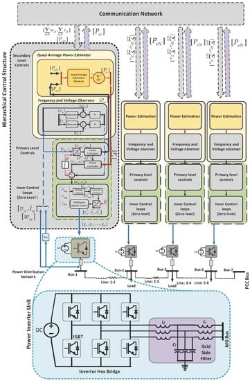
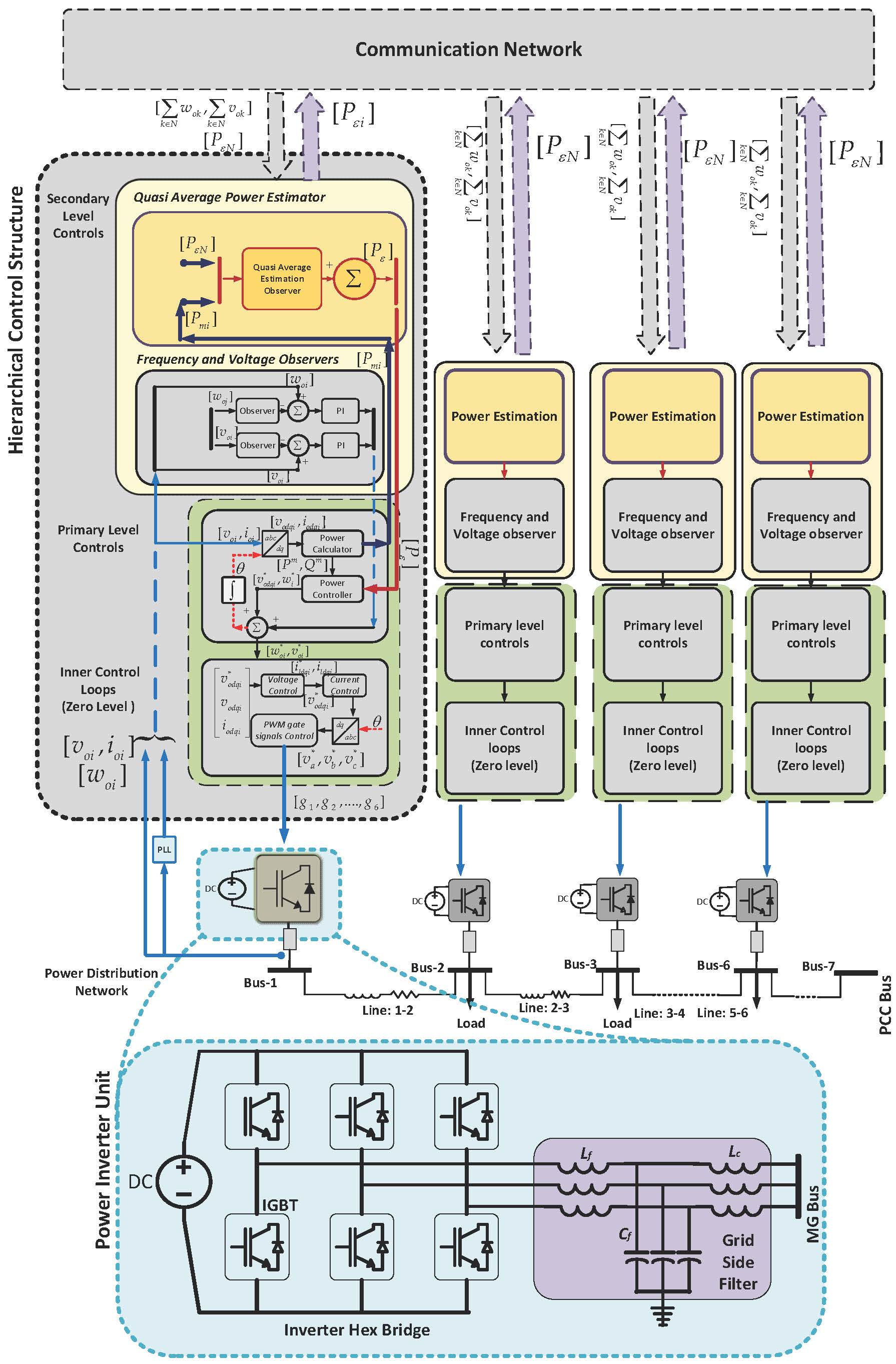
2.2. Hierarchical Control Structure and Information Exchange Media

The control scheme for the microgrid system is divided into a hierarchical control structure composed of three broad layers, graphically represented in Figure 1: the inner or zero level control loops are dedicated to regulating voltage and current loops for each power converter, generating gate pulses to operate individual converter. The primary layer regulates power sharing using droop control technique with the droop gains selected as (m_P*, n_Q*). The secondary/tertiary layer is composed of power, voltage and frequency observers that estimate these parameters based on information from neighborhood nodes (${{\displaystyle \sum }}_{k\in N}{\omega }_{oi}, {{\displaystyle \sum }}_{k\in N}{v}_{oi}, {{\displaystyle \sum }}_{k\in N}{P}_{\epsilon i}$), thereby providing regular corrective updates for power injection, voltage and frequency values (P_refi, ω_ni, V_ni) to maintain these within an agreeable range on a system wide scale. The communication network layer serves as the media for measured/estimated values and control signals to travel through the control system based on connectivity structure. For modelling and control design the connectivity between system nodes can be mapped as a digraph. A digraph is represented mathematically as $G_{com}=(V_g E_g A_g)$, which is composed of a non-empty, finite set of M nodes represented by $V_g=\{v_1 v_2 v_3\dots v_M\}$. The arcs that link these nodes are given by $E_g\subset V_g\times V_g$. The adjacency matrix representing the mapping and interconnection of different nodes through these arcs is given by $A_g=[a_{ij}]\in R^{N\times N}$. The DGUs can be considered as the nodes of a communication digraph, whereas the arcs show communication links [40]. Figure 2a details the interaction between primary and secondary control layers at a single node. Voltage and frequency corrections (ω_ni, V_ni) are generated through observer consensus based on global voltage and frequency references $(v_{ref},{\omega }_{ref})$ as well as neighborhood estimates $(v_{oj}, {\omega }_{oj})$. The third component estimates injected power average reference (P_refi), based on neighbor estimates $(\epsilon P_{avg.N})$, as later elaborated mathematically in Section 3.

An initially stable communication network is assumed for convenience that may be described as a time invariant digraph, as represented in Figure 2b, where the solid bi-directional arrows represent healthy communication links between DG nodes. Communication channel noise may be neglected for simplifying calculations. The resulting digraph is time invariant, i.e., $A_g$ is a constant. An arc emanating from node j and leading to node i is denoted by $(v_j, v_i)$, where node j receives information from node i. a_ij represents the weight of the arc connecting v_i to v_j. $a_{ij}>0$ if $(v_j, v_i)\in E_g$, otherwise $a_{ij}=0$. Node i is called a neighbor of node j if the arc $(v_j, v_i)\in E_g$. Set of nodes neighboring the i^th DGU $v_i$ are given by $N_i=\{v_j\in V_g:(v_i, v_j)\in E_g\}$. The Laplacian matrix, $L_g={(l_{ij})}_{N\times N}$ is defined as $l_{ij}=-a_{ij}, i\ne j$ and $l_{ii}={{\displaystyle \sum }}_{j-1}^N{a}_{ij} for i=1,\dots ., N.$ Such that $L_{1N}=0$ with $1_N={(1,\dots ,1)}^T\in R^N$. The in-degree matrix can be defined as $D_G^{in}=diag\{d_i^{in}\}$, where, $d_i^{in}={{\displaystyle \sum }}_{j\in N_i}(a_{ji})$ and out-degree matrix as $D_G^{out}=diag\{d_i^{out}\}$, where $d_i^{out}={{\displaystyle \sum }}_{i\in N_i}(a_{ji})$.

Multiagent consensus-based algorithms implemented across the networked control system cause system states $x$ to converge over a span of time and this can be represented as (4), (5).

$$\dot{x}=-C({\mathit{D}}_{\mathit{g}}-{\mathit{A}}_{\mathit{g}})x=-C{\mathit{L}}_{\mathit{g}}x$$

(4)

where,

$${\mathit{L}}_{\mathit{g}}={\mathit{D}}_{\mathit{g}}-{\mathit{A}}_{\mathit{g}}$$

(5)

Equation (5) represents the Laplacian matrix ${\mathit{L}}_{\mathit{g}}$ calculated for the communication network based on adjacency matrix ${\mathit{A}}_{\mathit{g}}$ and degree matrix ${\mathit{D}}_{\mathit{g}}$, $x$ represents the system states and $\dot{x}$ represents their evolved values as per the consensus algorithm, the factor C is a convergence factor whose value can be modeled based on network parameters [41]. The matrices A_g, D_g and L_g for the communication topology used are given in the Appendix B.

2.3. Network Latencies

Figure 2c represents the effect of communication latencies considered affecting three nodes, i.e., DG 1,6 and 5. The dotted lines represent communication links suffering from latencies whereas DGs are labelled 1 to 6 accordingly. The DG 6 is shown to be dually affected by communication health decay since all the links connecting it suffer from communication latencies. To elaborate upon the modelling of communication latencies, a networked control system can be described in discrete state space form as in (6):

$$\begin{array}{l}{x}_p(k+1)=A·x_p+B·u_p\\ y_p=C·x_p\end{array}\}.$$

(6)

where, matrices A, B and C represent a simplified form for state space matrices of a networked controlled system in discrete time, $x_p$ represents vector of system states considered in the modelling, $u_p$ are the inputs and $y_p$ are the outputs derived from the system. Assuming that a networked communication system is in place to relay the measured outputs, for a general case we may assume that all parameter measurements after passing through the communication network exhibit a randomly varying communication delay given by (7)

$$y_c(k)=y_p(k-\delta (k)·{\tau }_k^m).$$

(7)

where, ${\tau }_k^m$ represents the communication delay occurring at time instant k and $\delta \left(k\right)$ is a stochastic binary variable with $Prob\{\delta \left(k\right)=1\}=p_k$ where $p_k$ can take only discrete values [42]. In this work, for convenience in a larger system modeling, we approximate the communication delay ${\tau }_k^m$ with a uniform unit time delay represented by $t_d$ as in reference [41]. This delay is varied incrementally in discrete equal steps to emulate an increasing delay for different scenarios.

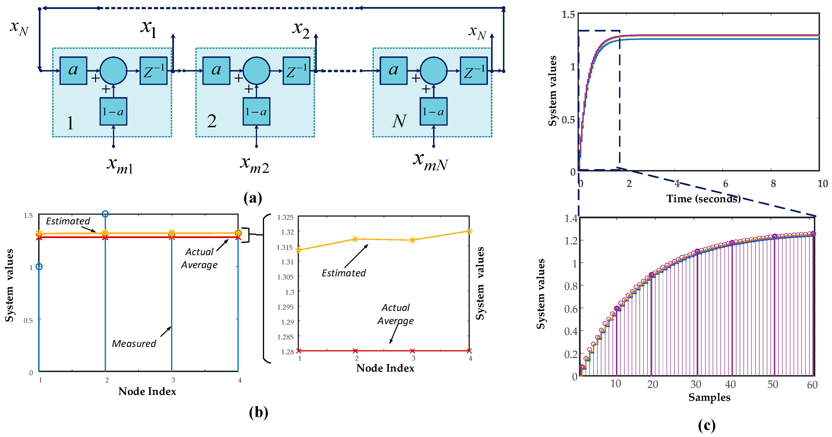
3. Distributed Quasi-average Estimation

Distributed multiagent control systems decompose the collective system average value estimation problem as a decentralized problem to be solved by every node (or agent). Consensus among participant agents can be achieved effectively when the communication network relays information and control signals with reasonable fidelity. However, with deteriorating communication link health, the average estimation convergence is affected [43]. As a solution to the adverse effects of communication intermittencies and faults, a new power sharing control is proposed, based on a distributed “quasi-average” estimation principle. Drawing inspiration from the theory and basics of infinite impulse response filters (IIR) [44], distributed quasi-average power estimators are programmed at every node as shown in Figure 3a and Figure 4c, that enable averaged values to be estimated. The structural interaction between averaging filters at each node is shown in Figure 3a. Each blue box represents the averaging filter at each node; node 1 to N are indicated accordingly. x_m1 through x_mN represent locally measured values, whereas x₁ through x_N represent average estimates, the term z⁻¹ represents a transmission unit delay of one processing cycle. All nodes converge at a “quasi-average” of values based on estimates received from neighboring nodes.

As an example, a simplified experiment given here shows the convergence of such quasi-average filters to values that are within an acceptable neighborhood of the true mean of measured values. A vector of real values is input to the system, $x_m=[1,1.5,1.3,1.32]$, where the first entry denotes $x_{m1}$, the second denotes $x_{m2}$, and so forth. The filter gain a is chosen within a range of (0.5 ≤ a ≤ 1), the estimates computed are influenced by the value of the filter gain chosen. For this experiment, a= 0.96 and the sampling time T = 1 × 10⁻³ seconds. Figure 3b shows the results of such an estimation for a simplified system of four nodes. the blue stems denote actual measured values, the yellow stars represent estimated values and the orange crosses denote actual mean value. Figure 3c shows results of time simulation of this filter study, while the magnified part shows value variation with each sample. It can be observed that there are minor differences between the actual mean value and the estimated averages, the major part of the average converges to the vicinity of the mean value, hence the term “quasi-average” has been used. In a feedback system, the controlled variable values are drawn towards the mean through the proposed control strategy.

These average estimates are used as references for localized droop control according to (8) as shown in Figure 4a, where frequency is proportionally reduced to create an offset from the common angular reference frame; this varies power injected by each unit and achieves active power sharing as shown by Equations (8) and (9).

$${\omega }_i^{*}={\omega }_i-m_{Pi}·(P_i-{\mathrm{P}}_{\mathsf{\epsilon }\mathrm{i}})$$

(8)

$$P_{\epsilon i}=x_{m·i}·(a)-x_{\epsilon N}·(1-a)·z^{-1}$$

(9)

where, a is the filter gain of quasi-average estimation observers, N is the number of nodes, i is the present node. $P_{\epsilon i}$ is the averaged power exchanged between nodes: $x_{\epsilon N}$ is the average received from the neighbor node, and $x_{mi}$ is the power measured at node i.

Elaboration: Distributed Estimation of Measured Power through Quasi-Average estimation

This section elaborates the proposed quasi-average estimation method by means of mathematical proof and deduction. Let the measured power at a node i, be represented by x_mi, while the estimate of the summation of all node injected powers received from neighboring nodes is given by x_ƹi. Assuming that measured values x_m are a constant vector of arbitrary values, as elaborated in Figure 3, the estimate of summations of powers calculated at nodes 1 and 2 can be given by (10) and (11) respectively

$$x_{\epsilon 1}(z)=0·x_1(z)z^{-1}+0·x_2(z)z^{-1}+‥+a·x_N(z)z^{-1}+b·x_{m1}(z)z^{-1}+0·x_{m2}(z)z^{-1}+‥+0·x_{mN}(z)z^{-1}$$

(10)

$$x_{\epsilon 2}(z)=a{x}_1(z)z^{-1}+0·x_2(z)z^{-1}+‥+0·x_N(z)z^{-1}+b·x_{m2}(z)z^{-1}+0·x_{m3}(z)z^{-1}+‥+0·x_{mN}(z)z^{-1}$$

(11)

We can write these equations for N nodes as (12) and (13)

$$\left[\begin{array}{c}{x}_{\epsilon 1}(z)\\ x_{\epsilon 2}(z)\\ .\\ x_{\epsilon N}(z)\end{array}\right]={\left[\begin{array}{cccc}& & & a\\ a& & & \\ & a& & \\ & & a& \end{array}\right]}_{N\times N}·z^{-1}·{\left[I\right]}_{N\times N}·\left[\begin{array}{c}{x}_{\epsilon (N-1)}(z)\\ x_{\epsilon 1}(z)\\ .\\ x_{\epsilon N}(z)\end{array}\right]+{\left[\begin{array}{cccc}b& & & \\ & .& & \\ & & .& \\ & & & b\end{array}\right]}_{N\times N}.z^{-1}.{\left[I\right]}_{N\times N}.\left[\begin{array}{c}{x}_{m1}(z)\\ x_{m2}(z)\\ .\\ x_{mN}(z)\end{array}\right]$$

(12)

$$\left[\begin{array}{c}{x}_{\epsilon 1}(z)\\ x_{\epsilon 2}(z)\\ .\\ x_{\epsilon N}(z)\end{array}\right]={\left[A\right]}_{N\times N}·z^{-1}·{\left[I\right]}_{N\times N}·\left[\begin{array}{c}{x}_{\epsilon (N-1)}(z)\\ x_{\epsilon 1}(z)\\ .\\ x_{\epsilon N}(z)\end{array}\right]+{\left[B\right]}_{N\times N}·z^{-1}·{\left[I\right]}_{N\times N}·\left[\begin{array}{c}{x}_{m1}(z)\\ x_{m2}(z)\\ .\\ x_{mN}(z)\end{array}\right]$$

(13)

where z⁻¹ represents a unit delay, and [I]_N×N represents an N by N Identity matrix converse with the number of N nodes of the system, the matrices [A]_N×N and [B]_N×N represent IIR filter gains for each node as in equation (13). Writing (13) and (14) in compact form as (14),

$${\left[x_{\epsilon }(z)\right]}_{N\times 1}={\left[A\right]}_{N\times N}·z^{-1}·{\left[I\right]}_{N\times N}·{\left[x_{\epsilon k}(z)\right]}_{N\times 1}+{\left[B\right]}_{N\times N}·z^{-1}·{\left[I\right]}_{N\times N}·{\left[x_m(z)\right]}_{N\times 1}$$

(14)

With mathematical manipulations (15), (16) and (17) may be obtained

$${\left[x_{\epsilon }(z)\right]}_{N\times 1}-{\left[A\right]}_{N\times N}·z^{-1}·{\left[I\right]}_{N\times N}·{\left[x_{\epsilon k}(z)\right]}_{N\times 1}={\left[B\right]}_{N\times N}·z^{-1}·{\left[I\right]}_{N\times N}·{\left[x_m(z)\right]}_{N\times 1}$$

(15)

$$\frac{{\left[x_{\epsilon }(z)\right]}_{N\times 1}-{\left[A\right]}_{N\times N}·z^{-1}·{\left[I\right]}_{N\times N}·{\left[x_{\epsilon k}(z)\right]}_{N\times 1}}{z^{-1}·{\left[I\right]}_{N\times N}}={\left[B\right]}_{N\times N}·{\left[x_m(z)\right]}_{N\times 1}$$

(16)

$$\frac{{\left[x_{\epsilon }(z)\right]}_{N\times 1}}{z^{-1}·{\left[I\right]}_{N\times N}}-{\left[A\right]}_{N\times N}·{\left[x_{\epsilon k}(z)\right]}_{N\times 1}={\left[B\right]}_{N\times N}·{\left[x_m(z)\right]}_{N\times 1}$$

(17)

For a system of N nodes,

$$[X_{\epsilon }(z)]=\frac{z(a-1)}{(a^4-1)}\left[\begin{array}{ccccc}1& a^{n-1}& a^{n-2}& .& a\\ a& 1& a^{n-1}& a^{n-2}& .\\ .& a& 1& a^{n-1}& a^{n-2}\\ a^{n-2}& .& a& 1& a^{n-1}\\ a^{n-1}& a^{n-2}& .& a& 1\end{array}\right]•\left[\begin{array}{c}{x}_{m1}(z)\\ x_{m2}(z)\\ .\\ x_{mN}(z)\end{array}\right]$$

(18)

Assume that we apply a constant input to each node, the steady state output can be obtained by final value theorem (19),

$$Li{m}_{k\to \infty }x[k]=Li{m}_{z\to 1}(z-1)x(z)$$

(19)

we can now write (20) and (21)

$$Li{m}_{Z\to 1}{\left[x_{\epsilon }(z)\right]}_{N\times 1}=Li{m}_{Z\to 1}(z^{-1}·{\left[I\right]}_{N\times N}-{\left[A\right]}_{N\times N})·({\left[B\right]}_{N\times N}·{\left[x_m(z)\right]}_{N\times 1})$$

(20)

$$[X_{\epsilon }]=\frac{(a-1)}{(a^4-1)}\left[\begin{array}{ccccc}1& a^{n-1}& a^{n-2}& .& a\\ a& 1& a^{n-1}& a^{n-2}& .\\ .& a& 1& a^{n-1}& a^{n-2}\\ a^{n-2}& .& a& 1& a^{n-1}\\ a^{n-1}& a^{n-2}& .& a& 1\end{array}\right]•\left[\begin{array}{c}{x}_{m1}\\ x_{m2}\\ .\\ x_{mN}\end{array}\right]$$

(21)

Assuming that, the values measured at every instant are the sum of system average values plus a marginal variation, we may write Equation (22)

$$\begin{array}{l}Let:x_{mi}={\overline{x}}_m+\Delta x_i\\ where\left\{\begin{array}{l}{\overline{x}}_m=\frac{{\displaystyle \sum \left\{x_{mi}\right\}}}{N}\\ i=1\to N\end{array}\right\}\end{array}$$

(22)

where N is the total number of nodes. By substituting (22) in (21), we have,

$$[X_{\epsilon }]=\frac{(a-1)}{(a^4-1)}\left[\begin{array}{ccccc}1& a^{n-1}& a^{n-2}& .& a\\ a& 1& a^{n-1}& a^{n-2}& .\\ .& a& 1& a^{n-1}& a^{n-2}\\ a^{n-2}& .& a& 1& a^{n-1}\\ a^{n-1}& a^{n-2}& .& a& 1\end{array}\right]•\left[\begin{array}{c}{\overline{x}}_{m1}+\Delta x\\ {\overline{x}}_{m2}+\Delta x\\ .\\ {\overline{x}}_{m4}+\Delta x\end{array}\right]$$

(23)

Considering a system of four nodes, the equations (23) yield the estimated averaged values as (24)

$$[X_{\epsilon }]=\frac{(a-1)}{(a^4-1)}\left[\begin{array}{cccc}1& a^3& a^2& a\\ a& 1& a^3& a^2\\ a^2& a& 1& a^3\\ a^3& a^2& a& 1\end{array}\right]•\left[\begin{array}{c}{\overline{x}}_{m1}+\Delta x\\ {\overline{x}}_{m2}+\Delta x\\ {\overline{x}}_{m3}+\Delta x\\ {\overline{x}}_{m4}+\Delta x\end{array}\right]$$

(24)

Simplifying for the matrix of estimated values, we may write

$$\begin{array}{l}[X_{\epsilon }]=[\begin{array}{ll}\frac{a^3({\overline{x}}_{m2}+\Delta x)\left(a-1\right)}{a^4}+\frac{({\overline{x}}_{m1}+\Delta x)\left(a-1\right)}{a^4}& \frac{a^3({\overline{x}}_{m3}+\Delta x)\left(a-1\right)}{a^4}+\frac{({\overline{x}}_{m2}+\Delta x)\left(a-1\right)}{a^4}+\\ +\frac{a^2({\overline{x}}_{m3}+\Delta x)\left(a-1\right)}{a^4}+\frac{a^{}({\overline{x}}_{m4}+\Delta x)\left(a-1\right)}{a^4}& \frac{a^{}({\overline{x}}_{m1}+\Delta x)\left(a-1\right)}{a^4}+\frac{a^2({\overline{x}}_{m4}+\Delta x)\left(a-1\right)}{a^4}\end{array}\\ \begin{array}{ll}\frac{a^3({\overline{x}}_{m4}+\Delta x)\left(a-1\right)}{a^4}+\frac{({\overline{x}}_{m3}+\Delta x)\left(a-1\right)}{a^4}& \frac{a^3({\overline{x}}_{m1}+\Delta x)\left(a-1\right)}{a^4}+\frac{({\overline{x}}_{m4}+\Delta x)\left(a-1\right)}{a^4}\\ +\frac{a^2({\overline{x}}_{m1}+\Delta x)\left(a-1\right)}{a^4}+\frac{a^{}({\overline{x}}_{m2}+\Delta x)\left(a-1\right)}{a^4}& +\frac{a^2({\overline{x}}_{m2}+\Delta x)\left(a-1\right)}{a^4}+\frac{a^{}({\overline{x}}_{m3}+\Delta x)\left(a-1\right)}{a^4}\end{array}{]}^T\end{array}$$

(25)

Following from these, we may write,

$$[x_{\epsilon }]=[{\overline{x}}_m]+[\Delta x_{\epsilon }].$$

(26)

where ${\overline{x}}_m$ is the average of measured values of power injected by each node into the system and Δx is the marginal variation in every measured value. The average power estimated at any node in the system converges to the major component of measured values ${\overline{x}}_m$ whereas the term Δx → 0 i.e., marginal variations tend towards zero. By approximation, we can say that the estimated value is nearly equal to the average of measured values:

$$x_{\epsilon }\cong {\overline{x}}_m$$

(27)

From the above elaborative analysis, it can be concluded that for a given value of a within a reasonable range, the proposed method accurately estimates a quasi-average value of measured power at every node in the system, within acceptable limits of being considered a nearly true average. As the proposed control is designed to operate in feedback, the system is collectively drawn towards an early convergence as shown in latter sections of this paper and further verified through system simulations. For synchrony in notation we may replace the terms x_ε by P_ε, representing active power average estimate and x_m by P_m, representing the measured active power. Therefore, Equations (26) and (27) can now be written as.

$$\left[P_{\epsilon i}\right]=\left[{\overline{P}}_{mi}\right]+\left[\Delta P_{\epsilon i}\right]$$

(28)

$$\left[P_{\epsilon i}\right]\cong \left[{\overline{P}}_{mi}\right]$$

(29)

4. Conventional Consensus Observers

For the sake of completeness, conventional consensus based observes are presented as an alternate for primary power sharing controller is described [20,45]. This method renders the average power reference P_εi through observation of previous measurements. Such an observer may be described as in (30).

$$P_{\epsilon i}(t)=P_i(t)+{\displaystyle {\int }_0^t{\displaystyle \sum _{j\in N_i}{a}_{ij}(\overline{P_j(\tau )}-\overline{P_i(}}}\tau ))·d\tau$$

(30)

Differentiating with respect to time, we obtain system dynamics

$$\overline{{\dot{P}}_{\epsilon i}}={\dot{P}}_i+{\displaystyle \sum _{j\in N_i}{a}_{ij}}({\overline{P}}_j-{\overline{P}}_i)={\dot{P}}_i+{\displaystyle \sum _{j\in N_i}{a}_{ij}{\overline{P}}_j-}{d}_i^{in}{P}_i$$

(31)

The system-wide observer dynamics may therefore be formulated as (32) and (33).

$${\overline{P}}_{\epsilon i}={\dot{P}}_i+A_G·{\overline{P}}_i-D_G^{in}·{\overline{P}}_i={\dot{P}}_i-(D_G^{in}-A_G)·{\overline{P}}_i$$

(32)

$${\overline{P}}_{\epsilon i}={\dot{P}}_i-L_G·{\overline{P}}_i$$

(33)

where (33) gives the dynamics of the decentralized power estimator used as a comparison benchmark tool to evaluate and verify the effectiveness of the proposed scheme.

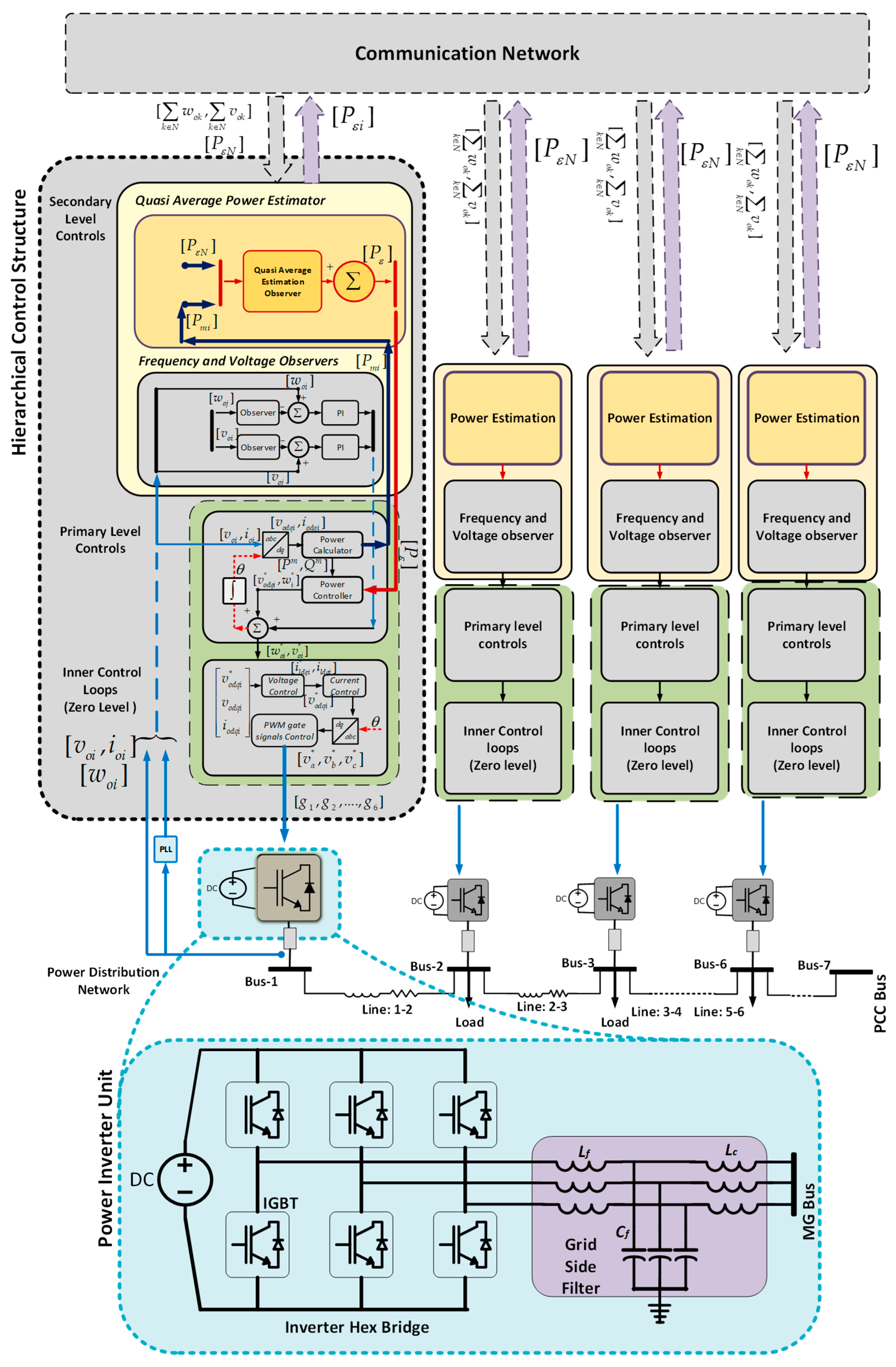
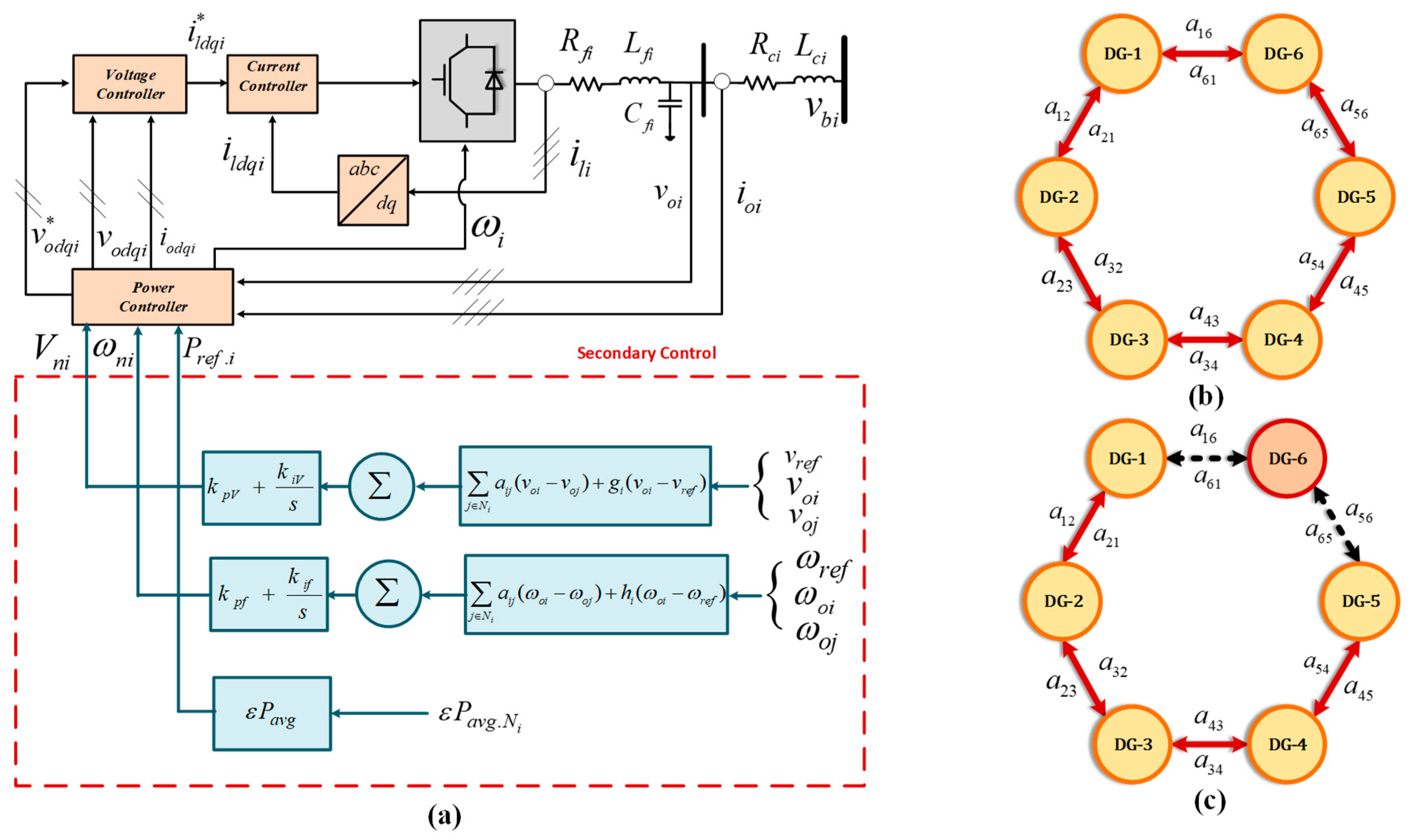
5. Secondary Regulation: Frequency and Voltage

Multiagent consensus-based controls are used for the secondary restoration of voltage magnitude and frequency [40]. Figure 2a shows the distributed voltage frequency and voltage restoration control scheme.

Frequency regulation controls can be given as (34).

$$\begin{array}{c}\delta {\omega }_i(k+1)=k_{pf}{e}_{\omega i}(k)+k_{if}{\displaystyle \sum _{i=ko}^k{e}_{\omega i}}(k)\\ e_{\omega i}(k+1)={\displaystyle \sum _{j\in N_i}{a}_{ij}\left({\omega }_{oi}(k)-{\omega }_{oj}(k)\right)+}{h}_i\left({\omega }_{oi}(k)-{\omega }_{ref}(k)\right)\end{array}\}$$

(34)

where, ${\omega }_{ref}^{}$ represents the angular frequency reference, ${\omega }_{oj}$ is the measured angular frequency at nodes in proximity of the i^th node. The terms k_pf and k_if are proportional gain and integral gain as seen in Figure 2a. $\delta {\omega }_i$ is the correction factor applied to frequency reference of the i^th inverter node. $h_i$ is the pinning gain whose value is zero for the primary node. The voltage regulation method can be described by (35):

$$\begin{array}{c}\delta V_i(k+1)=k_{pv}{e}_{vi}(k)+k_{iv}{\displaystyle \sum _{i=ko}^k{e}_{vi}}(k)\\ e_{vi}(k+1)={\displaystyle \sum _{j\in N_i}{a}_{ij}\left(v_{oi}(k)-v_{oj}(k)\right)+}{h}_i\left(v_{oi}(k)-v_{ref}(k)\right)\end{array}\}$$

(35)

where, $v_{nom}^{}$ is the nominal reference voltage in p.u. for the system, $v_{oj}$ is the voltage measured at all nodes in the communication neighborhood of the node i being considered. The terms k_pv and k_iv represent proportional and integral gains as shown in Figure 2a. $\delta V_i$ is the voltage correction term applied to the i^th inverter node. $g_i$ is the pinning gain, whose value is zero for the principal node.

6. Small Signal Model of the Microgrid System

Small signal models are derived for the MG system as shown in Figure 1. Component-wise state space models of the MG system are described in terms of matrices A, B, C and D [41,42,46]. Dynamical equations for the system are perturbed to obtain a corresponding small signal model of the MG system. This section elaborates each one of the model components used in development and analysis of the proposed control scheme.

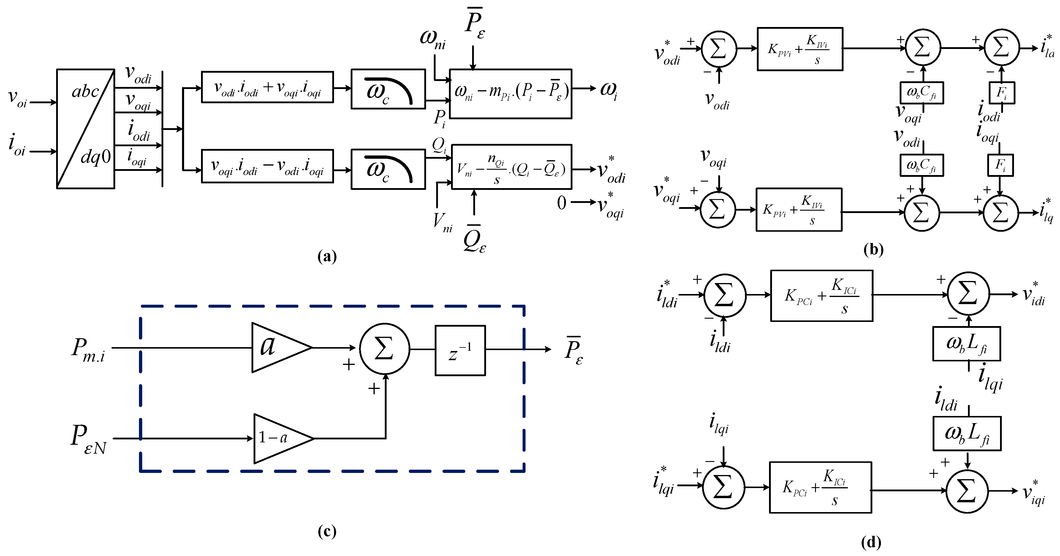
6.1. Fundamental/Zero Level Controls

Voltage and current controls formulated in d-q-0 frame amount to localized, “zero-level” control loops for each of the power converter units as elaborated in Figure 4b,d. Small signal equations for voltage control loop are given as (36) (37), are obtained by perturbing respective dynamical equations around quiescent point [47,48].

$$\left[\Delta {\dot{\varphi }}_{dq}\right]=\left[0\right]·\left[\Delta {\varphi }_{dq}\right]+B_{V1}·\left[\Delta v_{odq}^{*}\right]+B_{V2}·\left[\begin{array}{c}\Delta i_{ldq}\\ \Delta v_{odq}\\ \Delta i_{odq}\end{array}\right]$$

(36)

where,

$$\Delta {\varphi }_{dq}={\left[\begin{array}{cc}\Delta {\varphi }_d& \Delta {\varphi }_q\end{array}\right]}^T{B}_{v1}=\left[\begin{array}{cc}1& 0\\ 0& 1\end{array}\right],B_{v2}=\left[\begin{array}{cccccc}0& 0& -1& 0& 0& 0\\ 0& 0& 0& -1& 0& 0\end{array}\right]$$

and

$$\Delta i_{ldq}^{*}=C_V·\left[\Delta {\varphi }_{dq}\right]+D_{V1}\Delta v_{odq}^{*}+D_{V2}·\left[\begin{array}{c}\Delta i_{ldq}\\ \Delta v_{odq}\\ \Delta i_{odq}\end{array}\right]$$

(37)

where,

$$C_V=\left[\begin{array}{cc}{K}_{IVi}& 0\\ 0& K_{IVi}\end{array}\right],D_V=\left[\begin{array}{cc}{K}_{PVi}& 0\\ 0& K_{PVi}\end{array}\right]D_{V2}=\left[\begin{array}{cccccc}0& 0& -K_{PVi}& -{\omega }_n{C}_f& F_i& 0\\ 0& 0& {\omega }_n{C}_f& -K_{PVi}& 0& F_i\end{array}\right]$$

where, K_PVi and K_IVi are the proportional gain and integral gain of the voltage controller. ${\varphi }_{di}$ and ${\varphi }_{qi}$ represent auxiliary state variables for these PI controllers. F_i is an output feed-back gain. v_oqi, v_oid, i_odi and i_oqi are system measurements as seen in Figure 4b,d.

Similarly, (38) (39) represent the small signal model for the current control loop at each node as shown in Figure 2d.

$$\left[\Delta {\dot{\varsigma }}_{dq}\right]=\left[0\right]·\left[\Delta {\varsigma }_{dq}\right]+B_{C1}·\left[\Delta {\varsigma }^{*}{}_{ldq}\right]+B_{C2}·\left[\begin{array}{c}\Delta i_{ldq}\\ \Delta v_{odq}\\ \Delta i_{odq}\end{array}\right]$$

(38)

where,

$$\Delta {\varsigma }_{dq}={\left[\begin{array}{cc}\Delta {\varsigma }_d& \Delta {\varsigma }_q\end{array}\right]}^T$$

$$B_{C1}=\left[\begin{array}{cc}1& 0\\ 0& 1\end{array}\right],B_{C2}=\left[\begin{array}{cccccc}-1& 0& 0& 0& 0& 0\\ 0& -1& 0& 0& 0& 0\end{array}\right]$$

And,

$$\Delta v_{idq}^{*}=C_C\left[\Delta {\varsigma }_{dq}\right]+D_{C1}\left[\Delta i_{ldq}^{*}\right]+D_{C2}\left[\begin{array}{c}\Delta i_{ldq}\\ \Delta v_{odq}\\ \Delta i_{odq}\end{array}\right]$$

(39)

where,

$$C_C=\left[\begin{array}{cc}{K}_{ICi}& 0\\ 0& K_{ICi}\end{array}\right],D_{C1}=\left[\begin{array}{cc}{K}_{PCi}& 0\\ 0& K_{PCi}\end{array}\right].D_{C2}=\left[\begin{array}{cccccc}-K_{PCi}& -{\omega }_n{L}_f& 0& 0& 0& 0\\ {\omega }_n{L}_f& -K_{PCi}& 0& 0& 0& 0\end{array}\right]$$

where, K_PCi and K_ICi represent the proportional gain and integral gain of the voltage controller respectively. ${\varsigma }_d$ and ${\varsigma }_q$ are auxiliary state variables for the PI controllers used. I_lqi and, I_ldi, are system measurements as seen in Figure 2a.

6.2. Primary Power Balancing Control

Power balancing controls operate at the primary control level as elaborated in Figure 4a. These can be written in mathematical form as (40) (41) that represent the droop controller.

$${\omega }_i^{*}={\omega }_i-m_{Pi}(P_{mi}-P_{\epsilon i})$$

(40)

$$\begin{array}{l}{V}_{di}^{*}=V_{di}-n_{Qi}·(Q_{mi}-Q_{\epsilon i})\\ V_{qi}^{*}=0\\ V_o^{*}=\sqrt{{(V_{di}^{*})}^2-{(V_{qi}^{*})}^2}\end{array}$$

(41)

where, ${\omega }_i$ and $V_0$ represent the nominal references for frequency and voltage of the i^th inverter. $P_i$, $Q_i$ correspond to active and reactive powers being injected by the i^th inverter at output terminals. is the power estimate generated through the proposed quasi-averaging method or alternatively through consensus-based estimators described in Section 4. ${\mathit{m}}_{\mathit{P}\mathit{i}}$ and ${\mathit{n}}_{Q\mathit{i}}$ are droop gains [23]. Primary control involves calculating power injected using two-axis theory. For accurately measuring the fundamental power component, low pass filters are used having a cut off frequency of ${\omega }_{ci}$. The corresponding linearized small signal equations for the power controllers can be written as given by (42). The power controller provides operating frequency for the DGU (ω_i), and reference voltage (v_odi* and v_oqi*) for voltage control loop. v_oqi* is set to zero [23].

$$\begin{array}{l}\left[\begin{array}{c}\Delta \dot{\delta }\\ \Delta \dot{P}\\ \Delta \dot{Q}\end{array}\right]=A_P·\left[\begin{array}{c}\Delta \delta \\ \Delta P\\ \Delta Q\end{array}\right]+B_P\left[\begin{array}{c}\Delta i_{ldq}\\ \Delta v_{odq}\\ \Delta i_{odq}\end{array}\right]+B_{Pwcom}\left[\Delta w_{com}\right]\\ \left[\begin{array}{c}\Delta w\\ \Delta v_{odq}^{*}\end{array}\right]=\left[\begin{array}{c}{C}_{Pw}\\ C_{Pv}\end{array}\right]·\left[\begin{array}{c}\Delta \delta \\ \Delta P\\ \Delta Q\end{array}\right]\end{array}$$

(42)

where,

$$A_P=\left[\begin{array}{ccc}0& -m_p& 0\\ 0& -{\omega }_c& 0\\ 0& 0& -{\omega }_c\end{array}\right],B_{Pcom}=\left[\begin{array}{c}-1\\ 0\\ 0\end{array}\right]B_P=\left[\begin{array}{cccccc}0& 0& 0& 0& 0& 0\\ 0& 0& {\omega }_c{I}_{od}& {\omega }_c{I}_{oq}& {\omega }_c{V}_{od}& {\omega }_c{I}_{oq}\\ 0& 0& {\omega }_c{I}_{oq}& -{\omega }_c{I}_{od}& -{\omega }_c{V}_{oq}& {\omega }_c{V}_{od}\end{array}\right]$$

$$C_{Pw}=\left[\begin{array}{ccc}0& -m_p& 0\end{array}\right]C_{Pv}=\left[\begin{array}{ccc}0& 0& -n_q\\ 0& 0& 0\end{array}\right]$$

where $I_{od}$, $I_{oq}$, $V_{od}$ and $V_{oq}$ represent steady state values of $i_{od}$, $i_{oq}$, $v_{od}$, $v_{oq}$ as in Figure 4b,d; ${\omega }_{ci}$ represents the cut-off frequency value for low pass filters employed in the power calculation.

The small signal model of frequency and voltage control are given by (43).

$$\begin{array}{c}\Delta \omega =-m_p·\Delta P\\ \Delta v_{od}^{*}=-n_q·\Delta Q\\ \Delta v_{oq}^{*}=0\end{array}\}$$

(43)

The reference frames of all inverters can be seen with reference to a common reference frame. The angle difference between i^th inverter and common frequency reference frame is shown as (44)

$$\delta =\int (\omega -{\omega }_{com})·dt$$

(44)

where, ${\omega }_{com}$ is the MG common frequency measured at any one point in the system. The linearized small signal model is given by (45).

$$\Delta \dot{\delta }=\Delta \omega -\Delta {\omega }_{com}=-m_p·\Delta P-\Delta {\omega }_{com}$$

(45)

where,

$$[\Delta P_{\epsilon i}]=[P_{\epsilon i}]-[{\overline{P}}_{mi}]$$

(46)

The fractional change in power is represented by the difference between measured and estimated values at any instant. $P_{\epsilon i}$ are estimates of active power flowing at node i and ${\overline{P}}_{mi}$ are averaged values of measured power calculated through the proposed averaging observers described in Section 3 Equations (30) and (31).

6.3. Secondary Controls

Secondary control law given in Section 5. Secondary frequency regulation can be given by:

$$\delta w_i=\delta w_{Ai}+\delta w_{Bi}$$

(47)

where,

$$\begin{array}{l}\delta w_{Ai}=-k_{pf}(w_{oi}(t)-w_{oj}(t))\\ \delta w_{Bi}=-k_{if}{\displaystyle \underset{o}{\overset{t}{\int }}(w_{oi}(\tau )-w_{oj}(\tau ))}·d\tau \end{array}$$

(48)

Assuming an information transmission delay of time t_d, the combined small signal model for frequency regulation can be modelled as per [41] and represented as.

$$\begin{array}{l}[\Delta \delta {\dot{w}}_{Ai}(t)]=-{[k_{pf}]}_{N\times N}[D_g][\Delta {\dot{w}}_{oi}(t)]+{[k_{pf}]}_{N\times N}[A_g][\Delta {\dot{w}}_{oj}(t-t_d)]\\ [\Delta \delta {\dot{w}}_{Bi}(t)]=-{[k_{if}]}_{N\times N}[D_g][\Delta w_{oi}(t)]+{[k_{if}]}_{N\times N}[A_g][\Delta w_{oj}(t-t_d)]\end{array}$$

(49)

where, the correction factor perturbations are given by

$$[\Delta \delta {\dot{w}}_i]=[\Delta \delta {\dot{w}}_{Ai}]+[\Delta \delta {\dot{w}}_{Bi}]$$

(50)

The perturbations in frequencies can be given by

$$[\Delta {\dot{w}}_{\epsilon i}]=[\Delta \delta {\dot{w}}_{Ai}]+[\Delta {\dot{w}}_i]$$

(51)

The secondary voltage regulation law can be given by

$$\delta v_{dqi}=\delta v_{Adqi}+\delta v_{Bdqi}$$

(52)

where,

$$\begin{array}{l}\delta v_{Adqi}=-k_{pf}(v_{odqi}(t)-v_{odqj}(t))\\ \delta v_{Bdqi}=-k_{if}{\displaystyle \underset{o}{\overset{t}{\int }}(v_{odqi}(\tau )-v_{odqj}(\tau ))}·d\tau \end{array}$$

(53)

Considering an information transmission delay of time t_d, the combined small signal model for voltage regulation can be given as

$$\begin{array}{l}[\Delta \delta {\dot{v}}_{Adqi}(t)]=-{[k_{pv}]}_{N\times N}[D_g][\Delta {\dot{v}}_{odqi}(t)]+{[k_{pv}]}_{N\times N}[A_g][\Delta {\dot{v}}_{odqj}(t-t_d)]\\ [\Delta \delta {\dot{v}}_{Bdqi}(t)]=-{[k_{iv}]}_{N\times N}[D_g][\Delta v_{odqi}(t)]+{[k_{iv}]}_{N\times N}[A_g][\Delta v_{odqj}(t-t_d)]\end{array}$$

(54)

The perturbations in voltage correction terms can be given as

$$[\Delta \delta {\dot{v}}_{dqi}]=[\Delta \delta {\dot{v}}_{Adqi}]+[\Delta \delta {\dot{v}}_{Bdqi}]$$

(55)

By adding perturbed correction terms $\left[\Delta \delta \dot{v_{dqi}}\right]$ to the voltage terms $[\Delta \dot{v_{dqi}]}$, we can describe the total variation in voltages by

$$[\Delta {\dot{v}}_{\epsilon dqi}]=[\Delta \delta {\dot{v}}_{dqi}]+[\Delta {\dot{v}}_{dqi}]$$

(56)

The variations in line and load currents as well as inverter parameters with these perturbations are now written as

$$\begin{array}{l}[\Delta {\dot{i}}_{lineDQ}]=A_{NET}[\Delta i_{lineDQ}]+B_{1NET}[\Delta {\dot{v}}_{\epsilon dqi}]+B_{1NET}[\Delta {\dot{w}}_{\epsilon i}]\\ [\Delta {\dot{i}}_{loadDQ}]=A_{LOAD}[\Delta i_{lineDQ}]+B_{1LOAD}[\Delta {\dot{v}}_{\epsilon dqi}]+B_{2LOAD}[\Delta {\dot{w}}_{\epsilon i}]\end{array}$$

(57)

Considering the perturbations, the variation in inverter parameters may be described as.

$$\begin{array}{l}[\Delta {\dot{x}}_{invi}]=A_{invi}[\Delta x_{invi}]+B_{invi}[\Delta {\dot{v}}_{\epsilon dqi}]+B_{iwcom}[\Delta {\dot{w}}_{\epsilon i}+\Delta w_{com}]\\ \left[\begin{array}{c}\Delta {\dot{w}}_{\epsilon i}+\Delta w_{com}\\ \Delta i_{oDQi}\end{array}\right]=\left[\begin{array}{c}{C}_{inv.wi}\\ C_{inv.Ci}\end{array}\right]·[\Delta x_{inv.i}]\end{array}$$

(58)

6.4. Inverter Grid-side Filters

The small signal model for the LC output filters is given as,

$$\left[\begin{array}{c}\Delta i_{ldq}\\ \Delta v_{odq}\\ \Delta i_{odq}\end{array}\right]=A_{LCL}\left[\begin{array}{c}\Delta i_{ldq}\\ \Delta v_{odq}\\ \Delta i_{odq}\end{array}\right]+B_{LCL1}\left[\Delta v_{idq}\right]+B_{LCL2}\left[\Delta v_{bdq}\right]+B_{LCL3}\left[\Delta \omega \right]$$

(59)

The input and output parameters, as seen in Figure 2d may be transformed to a common rotationg d-q-0 reference frame using a transformation matrix $T_{\gamma }$, rotating with angular frequency ${\omega }_{com}$ as described in (60) (61).

$$\left[\Delta i_{0DQ}\right]=\left[T_{\gamma }\right]·\left[i_{odq}\right]=\left[\begin{array}{cc}\cos (\delta )& -\sin (\delta )\\ \sin (\delta )& \cos (\delta )\end{array}\right]·\left[\Delta i_{odq}\right]+\left[\begin{array}{cc}-I_{od}.\cos (\delta )& -I_{od}.\sin (\delta )\\ I_{od}.\sin (\delta )& -I_{oq}\cos (\delta )\end{array}\right]·\left[\Delta \delta \right]$$

(60)

$$\left[\Delta v_{bdq}\right]=\left[T_{\gamma }{}^{-1}\right]·\left[u_{bDQ}\right]=\left[\begin{array}{cc}\cos \left(\delta \right)& \sin \left(\delta \right)\\ -\sin \left(\delta \right)& \cos \left(\delta \right)\end{array}\right]·\left[\Delta v_{bDQ}\right]+\left[\begin{array}{cc}-U_{bD}\sin \left(\delta \right)& -U_{bQ}\cos \left(\delta \right)\\ -U_{bD}\cos \left(\delta \right)& -U_{bQ}\sin \left(\delta \right)\end{array}\right]\left[\Delta \delta \right]$$

(61)

where, the transformation matrix is $[T_{\gamma }]=\left[\begin{array}{cc}\cos \left(\delta \right)& \sin \left(\delta \right)\\ -\sin \left(\delta \right)& \cos \left(\delta \right)\end{array}\right]$

6.5. Model of an Individual Inverter

The components in described previous sections in equations (36) to (61) can be combined to formulate a complete small signal model for the i^th distributed generation unit power inverter. This model can be written in suitable and compact form as (62).

$$\begin{array}{l}[\Delta {\dot{x}}_{invi}]=A_{invi}[\Delta x_{invi}]+B_{invi}[\Delta {\dot{v}}_{\epsilon dqi}]+B_{iwcom}[\Delta {\dot{w}}_{\epsilon i}+\Delta w_{com}]\\ \left[\begin{array}{c}\Delta {\dot{w}}_{\epsilon i}+\Delta w_{com}\\ \Delta i_{oDQi}\end{array}\right]=\left[\begin{array}{c}{C}_{inv.wi}\\ C_{inv.Ci}\end{array}\right]·[\Delta x_{inv.i}]\end{array}$$

(62)

where, the state vector is given as (63)

$$[\Delta x_{invi}]={\left[\Delta {\delta }_i\Delta P_i\Delta Q_i\Delta {\varphi }_{dqi}\Delta {\varsigma }_{dqi}\Delta i_{ldqi}\Delta v_{odqi}\Delta i_{odqi}\right]}^T$$

(63)

The matrices Ainvi, Binvi, Biwcom, Cinwi, Cinvci are provided in the Appendix A.

6.6. Combined Model of Inverters

A combined model for N power converters that are connected to the microgrid network is presented as in: (64) to (69).

$$\begin{array}{c}\left[\Delta x_{inv}\right]=A_{inv}·\left[\Delta x_{inv}\right]+B_{inv}·\left[\Delta v_{bDQ}\right]\\ \left[\Delta i_{oDQ}\right]=C_{invc}·\left[\Delta x_{inv}\right]\end{array}\}$$

(64)

where the state vector is,

$$\left[\Delta x_{inv}\right]={\left[\Delta x_{inv1}\Delta x_{inv2}\dots ‥\Delta x_{invN}\right]}^T$$

(65)

And the system matrices can be given as,

$$A_{inv}={\left[\begin{array}{cccc}{A}_{inv1}+B_{1wcom}{C}_{invw1}& & & \\ & A_{inv2}+B_{2wcom}{C}_{invw2}& & \\ & & .& \\ & & & A_{invN}+B_{Nwcom}{C}_{invwN}\end{array}\right]}_{13\times 13}$$

(66)

$$B_{inv}={\left[\begin{array}{cccc}{B}_{inv1}& B_{inv2}& .& B_{invN}\end{array}\right]}^T{}_{13\times 2m}$$

(67)

$$\left[\Delta v_{bDQ}\right]={\left[\begin{array}{cccc}\Delta v_{bDQ1}& \Delta v_{bDQ2}& ‥& \Delta v_{bDQN}\end{array}\right]}^T$$

(68)

$$C_{inv}=Diag{\left[\begin{array}{cccc}\left[C_{invc1}\right]& \left[C_{invc2}\right]& .& \left[C_{invcN}\right]\end{array}\right]}_{2s\times 13s}$$

(69)

6.7. Network and Load Model

A model for the distribution network and system loads is derived through Kirchhoff voltage and current laws and can be expressed in terms of line currents and node voltages as in (70), (71) and (72).

$$\begin{array}{l}[\Delta {\dot{i}}_{lineDQ}]=A_{NET}[\Delta i_{lineDQ}]+B_{1NET}[\Delta {\dot{v}}_{\epsilon dqi}]+B_{1NET}[\Delta {\dot{w}}_{\epsilon i}]\\ [\Delta {\dot{i}}_{loadDQ}]=A_{LOAD}[\Delta i_{lineDQ}]+B_{1LOAD}[\Delta {\dot{v}}_{\epsilon dqi}]+B_{2LOAD}[\Delta {\dot{w}}_{\epsilon i}]\end{array}$$

(70)

where,

$$\begin{array}{l}\Delta i_{lineDQ}={[\Delta i_{lineDQ1},\Delta i_{lineDQ2},\dots \Delta i_{lineDQN}]}^T\\ \Delta i_{loadDQ}={[\Delta i_{loadDQ1},\Delta i_{loadDQ2},\dots \Delta i_{loadDQp}]}^T\\ \Delta v_{bDQ}={[\Delta v_{bDQ1},\Delta v_{bDQ2},\dots \Delta v_{bDQN}]}^T\\ \Delta \omega =\Delta {\omega }_{com}\end{array}\}$$

(71)

and,

$$\begin{array}{l}{A}_{Net}=Diag{\left[\begin{array}{cccc}{A}_{Net1},& A_{Net2}& ‥& A_{NetN}\end{array}\right]}_{2N\times 2N}\\ B_{2Net}={\left[\begin{array}{cccc}{B}_{2Net1},& B_{2Net2}& .& B_{2NetN}\end{array}\right]}^T{}_{2N\times 1}\\ B_{1Net}={\left[\begin{array}{cccc}{B}_{1Net1},& B_{1Net2}& .& B_{1NetN}\end{array}\right]}^T{}_{2N\times 2m}\end{array}\}$$

(72)

6.8. Complete Model of Micro Grid

Individual component models can be combined to form a small signal model of the complete microgrid system as described by (73-77). The system used here is composed of s = 6 DGUs, n = 6 lines, p = 5 loads, m = 7 nodes. MATLAB Simulink and linear analysis tools have been used to process this complex system.

$$\left[\Delta v_{bDQ}\right]=R_N(M_{inv}[\Delta i_{oDQ}]+M_{Load}[\Delta \dot{i_{loadDQ}]}+M_{net}[\Delta \dot{i_{lineDQ}]})$$

(73)

where,

$$R_N={\left[\begin{array}{ccc}{r}_N& & \\ & \ddots & \\ & & r_N\end{array}\right]}_{2m\times 2n}$$

(74)

$$M_{inv}={\left[\begin{array}{cccc}1& & & \\ & 1& & \\ 0& 0& 0& 0\\ 0& 0& 0& 0\\ & & 1& \\ & & & 1\end{array}\right]}_{2m\times 2s},M_{net}={\left[\begin{array}{cccc}-1& & & \\ 0& -1& & \\ 1& 0& -1& \\ & 1& 0& -1\\ & & 1& 0\\ & & & 1\end{array}\right]}_{2m\times 2n}$$

(75)

$$M_{Load}={\left[\begin{array}{ccc}-1& & \\ & \ddots & \\ & & -1\end{array}\right]}_{2m\times 2p}$$

(76)

$$\left[\begin{array}{c}\Delta {\dot{x}}_{\epsilon inv}\\ \Delta {\dot{i}}_{\epsilon lineDQ}\\ \Delta {\dot{i}}_{\epsilon loadDQ}\end{array}\right]=A_{\epsilon MG}\left[\begin{array}{c}\Delta x_{\epsilon inv}\\ \Delta i_{\epsilon lineDQ}\\ \Delta i_{\epsilon loadDQ}\end{array}\right]$$

(77)

where, (77) represents the complete MG system used in this study expressed as a small signal model. The system matrix A_MG is given in the Appendix A.

7. Discretization of System Models

Consider continuous-time state space and output equations of the above described systems:

$$\begin{array}{l}\dot{x}(t)=A_{c.sys}.x(t)+B_{c.sys}.u(t)\\ y(t)=C_{c.sys}.x(t)+D_{c.sys}.u(t)\end{array}$$

(78)

where, A_csys, B_csys, C_csys and D_csys represent the continuous time representation of the MG systems. The discrete time state space representation of these equations takes the form:

$$\begin{array}{l}x((k+1)T)=G_d(T)x(kT)+H_d(T)u(kT)\\ y(kT)=C_{d}x(kT)+D_{d}u(kT)\end{array}$$

(79)

where, the matrices G_d, H_d,C_d,D_d are discrete-time counterparts for A_csys, B_csys, C_csys and D_csys matrices in continuous-time that can be obtained from (80)(81),and (82).

$$G(T)=e^{A_{c.sys}T}$$

(80)

$$H(T)=\left({\displaystyle {\int }_0^T{e}^{A_{c.sys}\lambda }d\lambda }\right)B_{c.sys}$$

(81)

$$\begin{array}{l}{C}_d=C_{c.sys}\\ D_d=D_{c.sys}\end{array}$$

(82)

The matrices G_d and H_d depend on sampling period T. If the sampling period T is fixed, the matrices are constant. Matrices C and D are constant matrices independent of the sampling period T [49]. For delay analyses, the time delays are considered to be greater than the sampling period and being integral multiples of the sampling period.

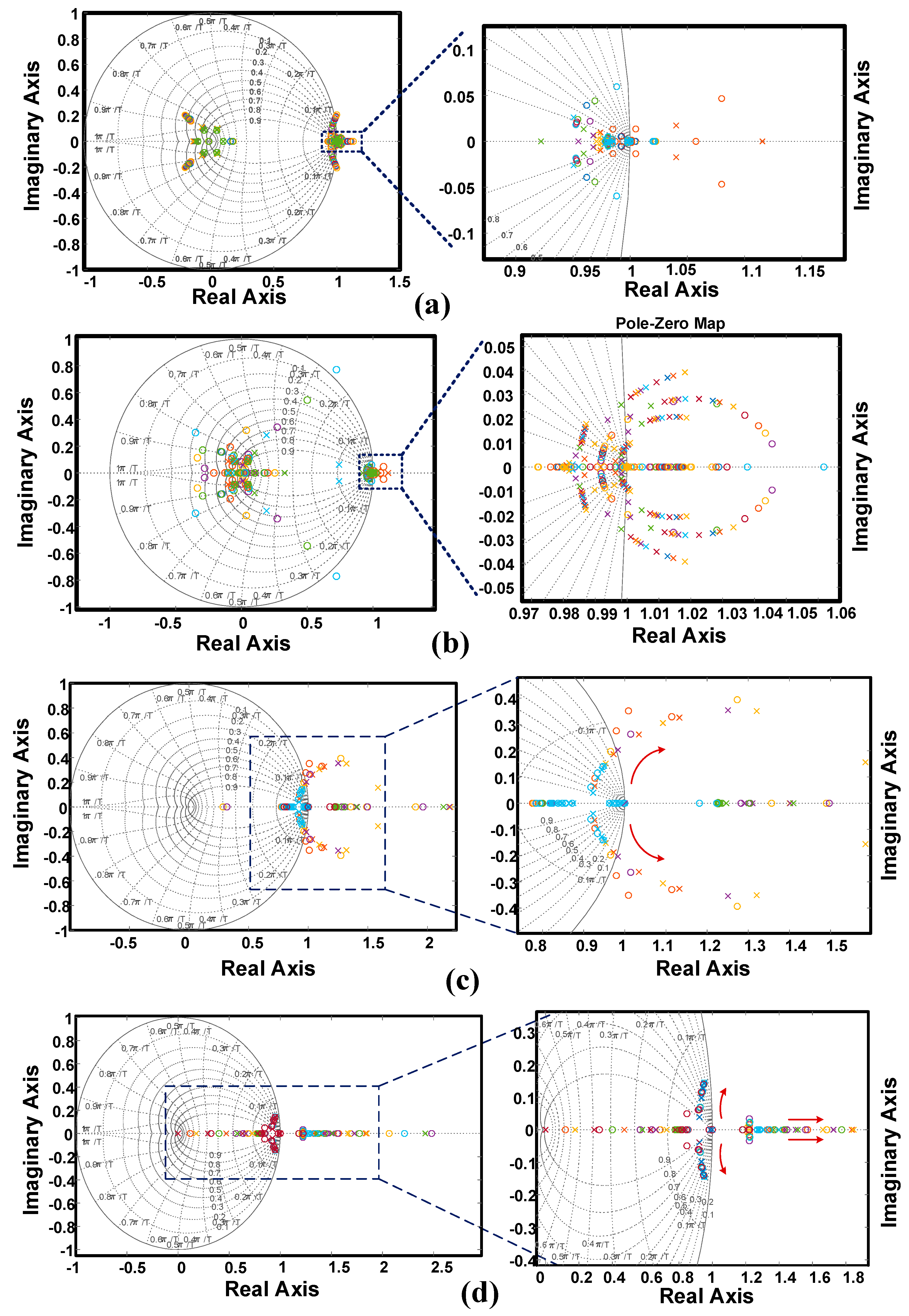
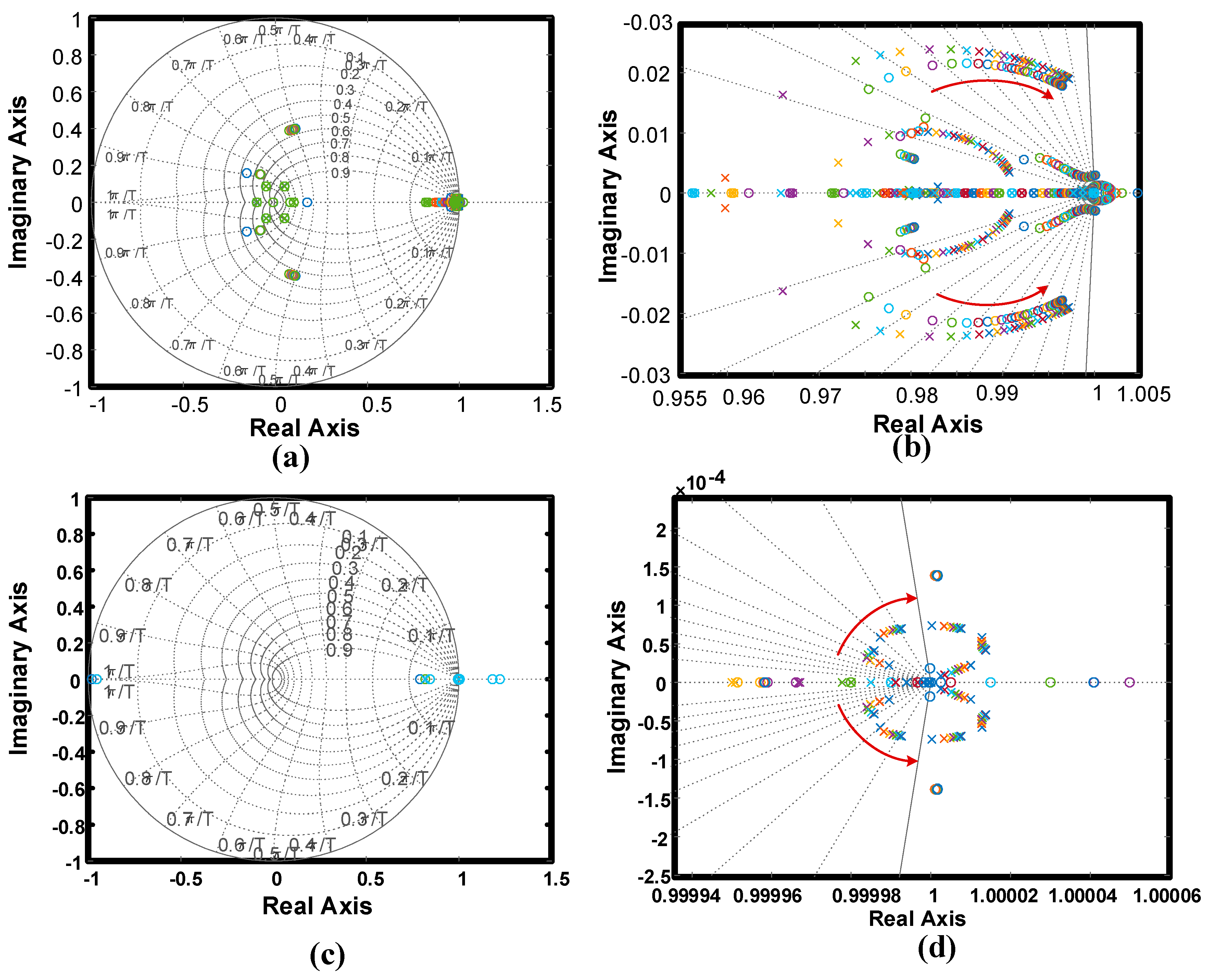
8. Stability Analysis Studies

A discrete time model of the MG system is presented here, outlined as (79-82). This model is used for system behavioral studies under different scenarios. The proposed averaging model is tested for different values of the IIR averaging gains $a$ and $b=(1-a)$. Furthermore, communication latencies and control gains are varied to plot the results. Thereby, limits are determined for control parameter variations. The droop gains of power sharing controllers (m_Pi, n_Qi) are varied to observe operational limits of the system. Communication time delays for selected link pairs connecting one system node (a₁₆, a₆₁) and (a₅₆, a₆₅) are varied incrementally to observe the effect produced on system poles and zeros.

Figure 5a–d elaborate the effect of incremental variations in reactive power control gains n_Qi and active power gains m_Pi. Figure 5a,b show the effect of varying m_Pi and n_Qi respectively under the proposed distributed power averaging method. For comparison, Figure 5c,d show the effect of variation in m_Pi and n_Qi under conventional consensus-based power sharing methods. With incrementally increasing control gains each successive plot shows the trend of movement in system poles and zeros. The control values (m_Pi, n_Qi), for which the system poles appear in the near vicinity of the unit origin are considered to be maximum allowable limits with regards to system stability. Therefore, system stability, sensitivity towards control gain and behavior are predicted using these pole-zero evolutions. In comparison with the conventional consensus-based power sharing approach, the proposed methodology adds more stability to the MG system under varying primary control gains. Among the two active and reactive power sharing gains, the system is more sensitive towards variations in reactive power gain n_Qi than m_Pi. the reactive power sharing controls therefore operate over a narrow margin.

Table 3. Variation Range for Controller Parameters.

Sr.No.	Control Parameters
1.	IIR gains	Min	Max
	a	0.5	0.98
	Droop Gains	Min	Max
	mp	1.0 × 10−10	1.0 × 10−3
	nq	1.0 × 10−7	1.0 × 10−3
2.	Consensus frequency
	kpf	0.4	2.5
	kif	0.1	0.5
3.	Consensus voltage
	kpV	0.5	3.5
	kiV	0.1	0.5
4.	Time Delay
	τdelay	0	5 s

outlines operational limits of control parameters obtained from the analysis.

Pole and zero traces given in Figure 6a,b, elaborate the behavior of this MG system under the influence of incrementally varying time delays with the proposed control scheme. Alternatively, Figure 6c,d elaborate the behavior of the proposed MG system under a conventional consensus-based power sharing approach for incrementally varying time delays. It can be inferred that in comparison with a consensus-based approach, the proposed distributed averaging-based method exhibits more system stability in the presence of communication latencies.

The consensus-based methods are integral methods that achieve consensus by collective error minimization. Communication latencies cause them to develop erroneous local estimates that magnify due to the integral effect of the controllers and the system values diverge. In comparison, the proposed error estimation method is resilient to errors resulting from delayed transmission of measurements and therefore results in a more robust control method that doesn’t diverge in the presence of communication latencies.

9. Case Study simulations

This section presents simulation studies undertaken in MATLAB and Simulink environment developed for stability studies. Possibilities resulting from multiple communication link latencies are considered. To emulate latencies, a time delay of 10ms to 5 seconds is introduced in the two links connecting DGU-6. The control algorithm subsequently strives to achieve equal power sharing along with voltage and frequency restoration. In comparison with consensus-based controls, the distributed average estimation method performs better. Even in the presence of large communication delays, the power sharing between nodes doesn’t significantly diverge. Whereas, in consensus-based methods, time delays lead to an observable divergence in controlled parameters.

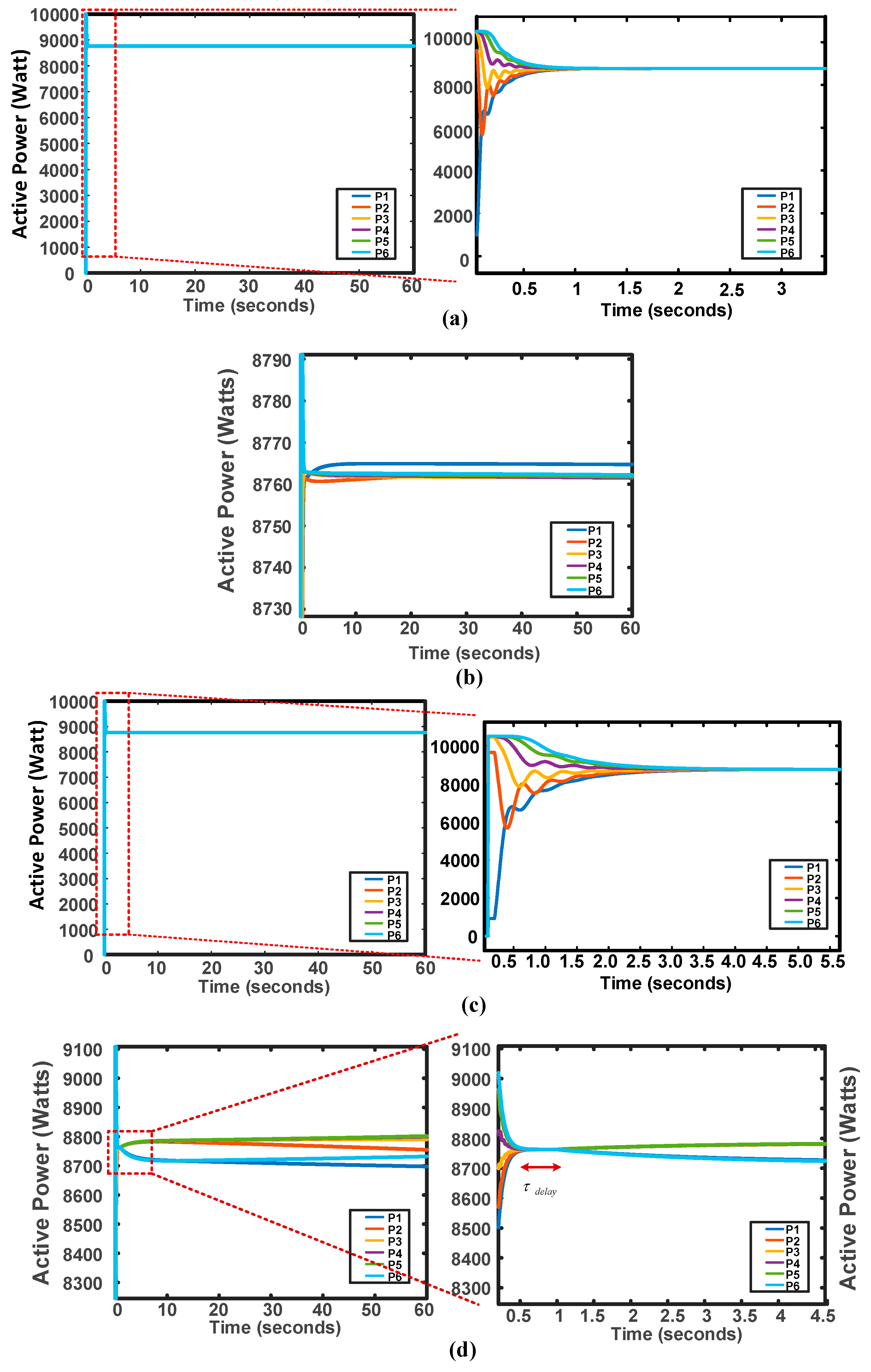
9.1. Active Power Sharing

Compared with a consensus observer-based approach given as (29), two scenarios are considered in this study: the first one has a communication network between nodes forming a complete ring digraph as represented in Figure 2b. All nodes receive information from at least two neighboring nodes. No communication latencies are considered at this stage. Figure 7a shows the results of power sharing with the proposed method and Figure 7b gives the results of power sharing with observer-based control for this scenario. The proposed method achieves power sharing more effectively as compared to the consensus-based method that exhibits measurable mismatch between active power injected by each node.

The second scenario considers dual link latencies leading to an isolated delay of information transmission directed towards and from DGU-6 as shown in Figure 2c. Figure 7c,d compare the results of power sharing under the proposed averaging based method and consensus observer-based control for this scenario. A divergence in injected powers can be observed in case of the consensus-based method. However, the proposed method achieves power sharing within finite time.

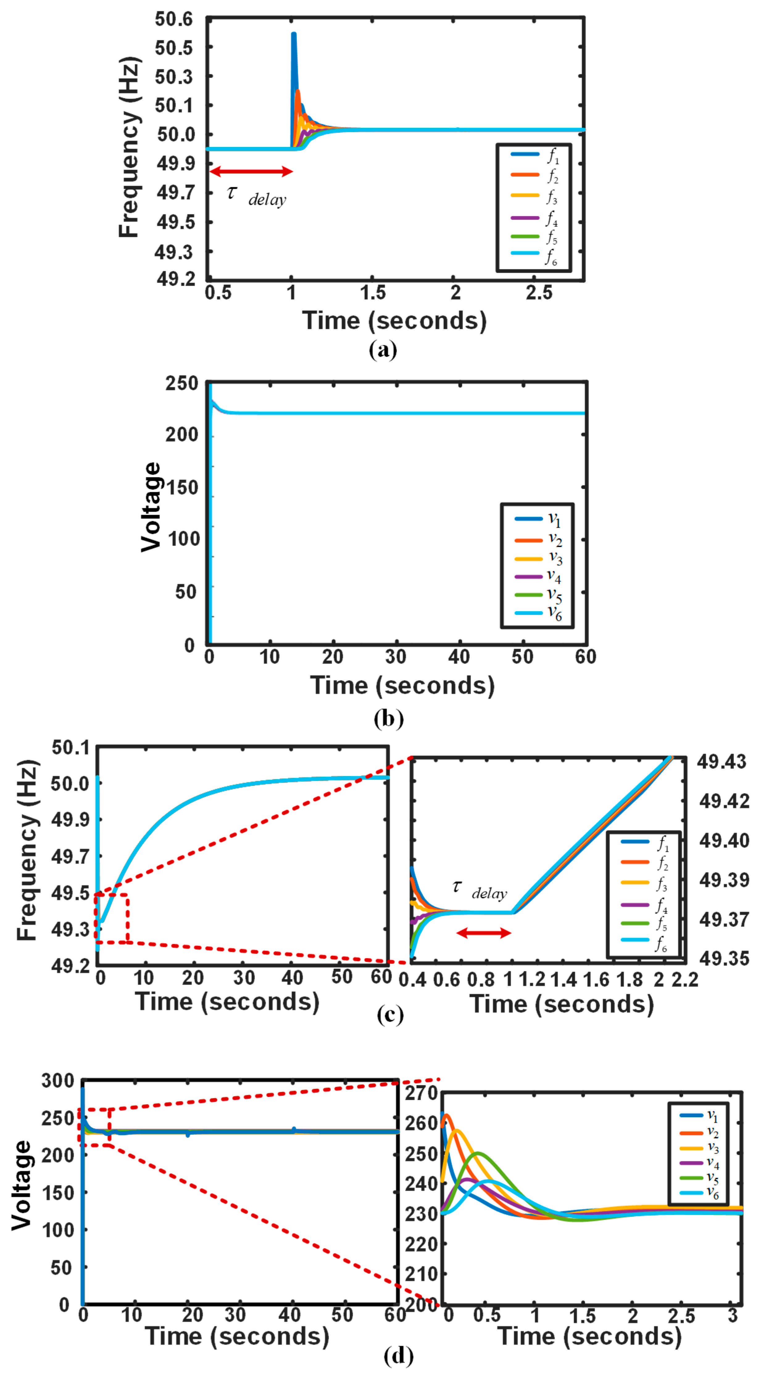
9.2. Frequency Regulation

This section compares the results of proposed frequency restoration method while working with distributed averaging-based power sharing and consensus-based power sharing schemes. Figure 8a shows the results of frequency restoration under the proposed power sharing method, whereas Figure 8c shows the result of frequency restoration under consensus observer-based method. A time delay can be observed in the presence of link latencies. With the proposed method, system frequency is restored to the desired value in a lesser time duration as compared with the consensus-based method.

9.3. Voltage Regulation

The proposed method is compared with consensus observer-based controls. Figure 8b represents voltage restoration under proposed method whereas, Figure 8d shows results of the observer-based scheme. Both methods achieve voltage restoration to desired values. However, the consensus observer-based scheme exhibits more divergence in node voltages during initial two seconds following the startup transient. Meanwhile, distributed power averaging-based method achieves voltage restoration without significant node voltage deviations during this initial time span.

For the proposed method, all converters in the system reach a consensus of corrective values for $P_{\epsilon i}$, $\delta {\omega }_i$ and $\delta V_i$, thereby, directing overall system power sharing, frequency and voltage to desired values within finite time. However, for the consensus observer-based method the system frequency and voltage take greater time to converge. Overall, the results show that the proposed method adds resilience towards communication delays, wherein accurate power sharing, voltage and frequency restoration is achieved within finite time.

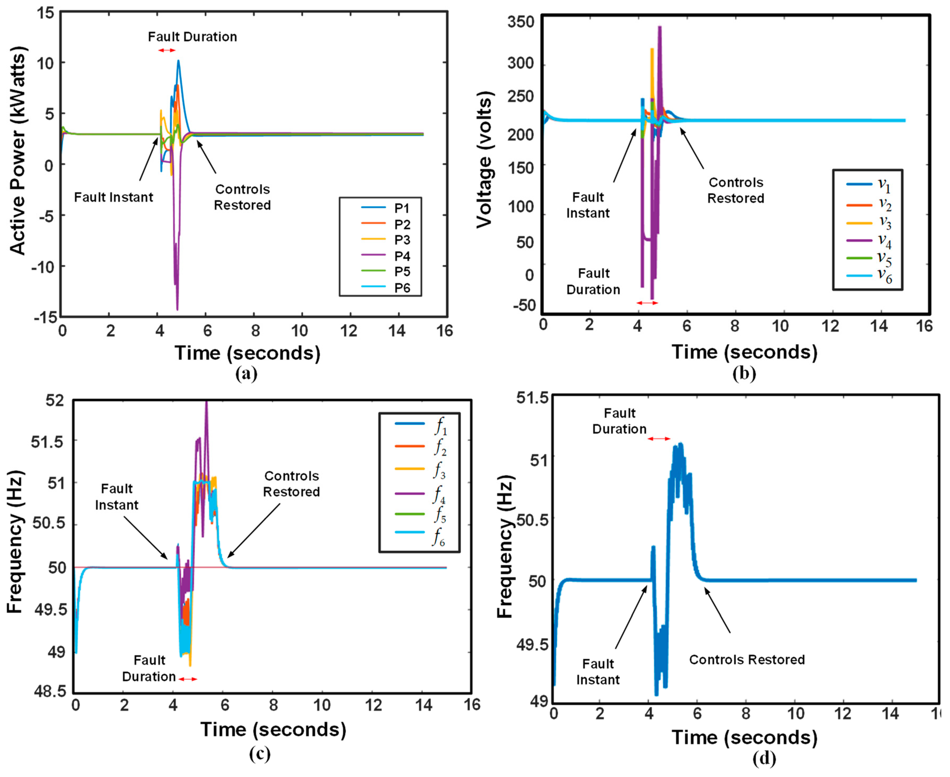
9.4. Performance of Controllers under Grid Faults

To present the performance of proposed controls under grid fault, a three-phase fault is introduced at bus-4 for a duration of 0.5 second. The fault parameters are given in

Table 4. Short Circuit Fault Parameters.

Sr.No.	Parameter	Value
1.	Fault Resistance
	Ron	0.001 Ω
2.	Ground Resistance
	Rg	0.01 Ω
3.	Snubber resistance
	Rs	1 × 10−6 Ω
4.	Snubber capacitance
	Cs	inf
5.	Short circuit type
	L-L-L-G

. The performance of primary active power sharing controls as well as frequency and voltage restoration secondary controls are presented in Figure 9. Figure 9a through 9c present the results of power sharing, voltage restoration, and frequency restoration. Whereas 9d shows frequency variations observed at PCC buss 7. It can be observed that once the fault is cleared the proposed controls rapidly recover system values to pre-fault levels.

10. Conclusions

An observer aided, decentralized and hierarchical control strategy has been proposed for power sharing between distributed generation units connected to an islanded AC micro-grid. Localized quasi-average power estimators based on the theory of IIR filters are employed to arrive at an estimate of instantaneous power being injected by each node. A multi-agent based secondary control for voltage and frequency regulation is implemented to observe and minimize deviations in key system parameters. A sparse communication network that links all DGUs in the MG system provides media for control signals to flow. The proposed distributed method stabilizes the MG system operation when this supervisory communication layer is experiencing link latencies. Discrete time mathematical small signal models of individual system components are combined to form an MG system model. This model is then used to analyze the performance of the proposed methodology using pole-zero evolutions with regards to system stability and sensitivity towards variations in control parameters. Simulation studies are undertaken to test the effectiveness of the proposed method. A comparison of the proposed method with conventional consensus-based control scheme reveals that the proposed strategy adds resilience to the system against control errors caused by communication link latencies. Even for large delays the system remains stable, which is in stark difference with purely consensus-based methods that show marked divergence in controlled variables once communication latencies are experienced. The mathematical stability analyses and simulation studies further verify the effectiveness of the proposed control methodology for the given scenarios.

References

1. Zeng, Z.; Yang, H.; Zhao, R. Study on small signal stability of microgrids: A review and a new approach. Renew. Sustain. Energy Rev. 2011, 15, 4818–4828. [Google Scholar] [CrossRef]
2. Han, Y.; Li, H.; Shen, P.; Coelho, E.A.A.; Guerrero, J.M. Review of Active and Reactive Power Sharing Strategies in Hierarchical Controlled Microgrids. IEEE Trans. Power Electron. 2017, 32, 2427–2451. [Google Scholar] [CrossRef]
3. Habib, S.; Khan, M.M.; Abbas, F.; Sang, L.; Shahid, M.U.; Tang, H. A Comprehensive Study of Implemented International Standards, Technical Challenges, Impacts and Prospects for Electric Vehicles. IEEE Access 2018, 6, 13866–13890. [Google Scholar] [CrossRef]
4. Hossain, M.A.; Pota, H.R.; Issa, W.; Hossain, M.J. Overview of AC microgrid controls with inverter-interfaced generations. Energies 2017, 10, 1300. [Google Scholar] [CrossRef]
5. Li, C.; Dragicevic, T.; Vasquez, J.C.; Guerrero, J.M.; Coelho, E.A.A. Multi-agent-based distributed state of charge balancing control for distributed energy storage units in AC microgrids. In Proceedings of the 2015 IEEE Applied Power Electronic Conference Exposition, Charllote, NC, USA, 15–19 March 2015; Volume 53, pp. 2967–2973. [Google Scholar] [CrossRef]
6. Ghanaatian, M.; Lotfifard, S. Control of Flywheel Energy Storage Systems in Presence of Uncertainties. IEEE Trans. Sustain. Energy 2018, 3029. [Google Scholar] [CrossRef]
7. Habib, S.; Kamran, M.; Rashid, U. Impact analysis of vehicle-to-grid technology and charging strategies of electric vehicles on distribution networks—A review. J. Power Sources 2015, 277, 205–214. [Google Scholar] [CrossRef]
8. Guan, Y.; Meng, L.; Li, C.; Vasquez, J.C.; Guerrero, J.M. Discharge rate balancing control strategy based on dynamic consensus algorithm for energy storage units in AC microgrids. In Proceedings of the IEEE Applied Power Electronics Conference and Exposition APEC, Tampa, FL, USA, 26–30 March 2017; pp. 2788–2794. [Google Scholar]
9. Li, H.; Han, Y.; Yang, P.; Xiong, J.; Wang, C.; Guerrero, J.M. A proportional harmonic power sharing scheme for hierarchical controlled microgrids considering unequal feeder impedances and nonlinear loads. In Proceedings of the IEEE Energy Conversion Congrgress Exposition ECCE, Cincinnati, OH, USA, 1–5 October 2017; pp. 3722–3727. [Google Scholar] [CrossRef]
10. Han, H.; Hou, X.; Yang, J.; Wu, J.; Su, M.; Guerrero, J.M. Review of power sharing control strategies for islanding operation of AC microgrids. IEEE Trans. Smart Grid 2016, 7, 200–215. [Google Scholar] [CrossRef]
11. Baghaee, H.R.; Mirsalim, M.; Gharehpetian, G.B. Power Calculation Using RBF Neural Networks to Improve Power Sharing of Hierarchical Control Scheme in Multi-DER Microgrids. IEEE J. Emerg. Sel. Top. Power Electron. 2016, 4, 1217–1225. [Google Scholar] [CrossRef]
12. Rokrok, E.; Golshan, M.E.H. Adaptive voltage droop scheme for voltage source converters in an islanded multibus microgrid. IET Gener. Transm. Distrib. 2010, 4, 562. [Google Scholar] [CrossRef]
13. Guerrero, J.M.; Matas, J.; de Vicuna, L.G.; Castilla, M.; Miret, J. Decentralized control for parallel operation of distributed generation inverters using resistive output impedance. IEEE Trans. Ind. Electron. 2007, 54, 994–1004. [Google Scholar] [CrossRef]
14. Guerrero, J.M.; De Vicuña, L.G.; Matas, J.; Miret, J.; Castilla, M. Output impedance design of parallel-connected UPS inverters. In Proceedings of the IEEE International Symposium Industrial Electronic, Ajaccio, France, 4–7 May 2004; Volume 2, pp. 1123–1128. [Google Scholar] [CrossRef]
15. Guerrero, J.M.; Matas, J.; De Vicuña, L.G.; Castilla, M.; Miret, J. Wireless-control strategy for parallel operation of distributed-generation inverters. IEEE Trans. Ind. Electron. 2006, 53, 1461–1470. [Google Scholar] [CrossRef]
16. Guerrero, J.M.; Vásquez, J.C.; Matas, J.; Castilla, M.; García de Vicuna, L. Control strategy for flexible microgrid based on parallel line-interactive UPS systems. IEEE Trans. Ind. Electron. 2009, 56, 726–736. [Google Scholar] [CrossRef]
17. De Brabandere, K.; Bolsens, B.; Van Den Keybus, J.; Woyte, A.; Driesen, J.; Belmans, R. A voltage and frequency droop control method for parallel inverters. In Proceedings of the IEEE 35th Annual Power Electronic Specialists Conference, Aachen, Germany, 20–25 June 2004; Volume 4, pp. 2501–2507. [Google Scholar] [CrossRef]
18. Alizadeh, E.; Birjandi, A.M.; Hamzeh, M. Decentralised power sharing control strategy in LV microgrids under unbalanced load conditions. IET Gener. Transm. Distrib. 2017, 11, 1613–1623. [Google Scholar] [CrossRef]
19. Xia, Y.; Peng, Y.; Wei, W. Triple droop control method for ac microgrids. IET Power Electron. 2017, 10, 1705–1713. [Google Scholar] [CrossRef]
20. Bidram, A.; Nasirian, V.; Davoudi, A.; Lewis, F.L. Droop-free distributed control of AC microgrids. In Cooperative Synhronization in Disturbed Microgrid Control; Springer International Publishing: New York, NY, USA, 2017; Volume 31, pp. 141–171. [Google Scholar] [CrossRef]
21. Guerrero, J.M.; Chandorkar, M.; Lee, T.L.; Loh, P.C. Advanced control architectures for intelligent microgridspart i: Decentralized and hierarchical control. IEEE Trans. Ind. Electron. 2013, 60, 1254–1262. [Google Scholar] [CrossRef]
22. Shahid, M.U.; Hashmi, K.; Habib, S.; Mumtaz, M.A.; Tang, H. A Hierarchical Control Methodology for Renewable DC Microgrids Supporting a Variable Communication Network Health. Electronics 2018, 7, 418. [Google Scholar] [CrossRef]
23. Bidram, A.; Member, S.; Davoudi, A.; Lewis, F.L.; Guerrero, J.M.; Member, S. Distributed Cooperative Secondary Control of Microgrids Using Feedback Linearization. IEEE Trans. Power Electron. 2013, 28, 3462–3470. [Google Scholar] [CrossRef] [Green Version]
24. Lu, L.Y.; Chu, C.C. Consensus-Based Secondary Frequency and Voltage Droop Control of Virtual Synchronous Generators for Isolated AC Micro-Grids. IEEE J. Emerg. Sel. Top. Circuits Syst. 2015, 5, 443–455. [Google Scholar] [CrossRef]
25. Wang, X.; Zhang, H.; Li, C. Distributed finite-time cooperative control of droop-controlled microgrids under switching topology. IET Renew. Power Gener. 2017, 11, 707–714. [Google Scholar] [CrossRef]
26. Sanjari, M.J.; Gharehpetian, G.B. Unified framework for frequency and voltage control of autonomous microgrids. IET Gener. Transm. Distrib. 2013, 7, 965–972. [Google Scholar] [CrossRef]
27. Lewis, F.L.; Qu, Z.; Davoudi, A.; Bidram, A. Secondary control of microgrids based on distributed cooperative control of multi-agent systems. IET Gener. Transm. Distrib. 2013, 7, 822–831. [Google Scholar] [CrossRef]
28. Liu, W.; Gu, W.; Xu, Y.; Wang, Y.; Zhang, K. General distributed secondary control for multi-microgrids with both PQ-controlled and droop-controlled distributed generators. IET Gener. Transm. Distrib. 2017, 11, 707–718. [Google Scholar] [CrossRef]
29. Zuo, S.; Davoudi, A.; Song, Y.; Lewis, F.L. Distributed Finite-Time Voltage and Frequency Restoration in Islanded AC Microgrids. IEEE Trans. Ind. Electron. 2016, 63, 5988–5997. [Google Scholar] [CrossRef]
30. Guo, F.; Wen, C.; Mao, J.; Song, Y.D. Distributed Secondary Voltage and Frequency Restoration Control of Droop-Controlled Inverter-Based Microgrids. IEEE Trans. Ind. Electron. 2015, 62, 4355–4364. [Google Scholar] [CrossRef]
31. Lu, X.; Yu, X.; Lai, J.; Guerrero, J.M.; Zhou, H. Distributed Secondary Voltage and Frequency Control for Islanded Microgrids With Uncertain Communication Links. IEEE Trans. Ind. Inform. 2017, 13, 448–460. [Google Scholar] [CrossRef] [Green Version]
32. Wang, Y.; Wang, X.; Chen, Z.; Blaabjerg, F. Distributed optimal control of reactive power and voltage in islanded microgrids. IEEE Trans. Ind. Appl. 2017, 53, 340–349. [Google Scholar] [CrossRef]
33. Hashmi, K.; Khan, M.M.; Habib, S.; Tang, H. An Improved Control Scheme for Power Sharing between Distributed Power Converters in Islanded AC Microgrids. In Proceedings of the International Conference on Frontiers of Information Technology, Islamabad, Pakistan, 18–20 December 2017; pp. 270–275. [Google Scholar] [CrossRef]
34. Schiffer, J.; Seel, T.; Raisch, J.; Sezi, T. Voltage Stability and Reactive Power Sharing in Inverter-Based Microgrids with Consensus-Based Distributed Voltage Control. IEEE Trans. Control Syst. Technol. 2016, 24, 96–109. [Google Scholar] [CrossRef]
35. Han, Y.; Zhang, K.; Li, H.; Coelho, E.A.A.; Guerrero, J.M. MAS-Based Distributed Coordinated Control and Optimization in Microgrid and Microgrid Clusters: A Comprehensive Overview. IEEE Trans. Power Electron. 2018, 33, 6488–6508. [Google Scholar] [CrossRef] [Green Version]
36. Hashmi, K.; Mansoor Khan, M.; Jiang, H.; Umair Shahid, M.; Habib, S.; Talib Faiz, M.; Tang, H. A Virtual Micro-Islanding-Based Control Paradigm for Renewable Microgrids. Electronics 2018, 7, 105. [Google Scholar] [CrossRef]
37. Guan, Y.; Meng, L.; Li, C.; Vasquez, J.; Guerrero, J. A Dynamic Consensus Algorithm to Adjust Virtual Impedance Loops for Discharge Rate Balancing of AC Microgrid Energy Storage Units. IEEE Trans. Smart Grid 2017, 9, 4847–4860. [Google Scholar] [CrossRef]
38. Shahid, M.U.; Khan, M.M.; Hashmi, K.; Habib, S.; Jiang, H.; Tang, H. A Control Methodology for Load Sharing System Restoration in Islanded DC Micro Grid with Faulty Communication Links. Electronics 2018, 7, 90. [Google Scholar] [CrossRef]
39. Khan, M.; Khan, M.; Jiang, H.; Hashmi, K.; Shahid, M. An Improved Control Strategy for Three-Phase Power Inverters in Islanded AC Microgrids. Inventions 2018, 3, 47. [Google Scholar] [CrossRef]
40. Bidram, A.; Nasirian, V.; Davoudi, A.; Lewis, F.L. Cooperative Synchronization in Distributed Microgrid Control, 1st ed.; Grimble, M.J., Ed.; Springer International Publishing: New York, NY, USA, 2017; ISBN 978-3-319-50807-8. [Google Scholar]
41. Coelho, E.A.A.; Wu, D.; Guerrero, J.M.; Vasquez, J.C.; Dragičević, T.; Stefanović, Č.; Popovski, P. Small-Signal Analysis of the Microgrid Secondary Control Considering a Communication Time Delay. IEEE Trans. Ind. Electron. 2016, 63, 6257–6269. [Google Scholar] [CrossRef] [Green Version]
42. Mahmoud, M.S.; AL-Sunni, F.M. Control and Optimization of Distributed Generation Systems, 1st ed.; Springer International Publishing: New York, NY, USA, 2015; ISBN 978-3-319-16909-5. [Google Scholar]
43. Schiffer, J.; Dörfler, F.; Fridman, E. Robustness of distributed averaging control in power systems: Time delays & dynamic communication topology. Automatica 2017, 80, 261–271. [Google Scholar] [CrossRef] [Green Version]
44. Shenoi, B.A. Introduction to Digital Signal Processing and Filter Design, 1st ed.; John Wiley & Sons: Hoboken, NJ, USA, 2006; ISBN 13 978-0-471-46482-2. [Google Scholar]
45. Nasirian, V.; Moayedi, S.; Davoudi, A.; Lewis, F.L. Distributed cooperative control of dc microgrids. IEEE Trans. Power Electron. 2015, 30, 2288–2303. [Google Scholar] [CrossRef]
46. Mariani, V.; Vasca, F.; Vasquez, J.C.; Guerrero, J.M. Model Order Reductions for Stability Analysis of Islanded Microgrids With Droop Control. IEEE Trans. Ind. Electron. 2015, 62, 4344–4354. [Google Scholar] [CrossRef] [Green Version]
47. Pogaku, N.; Prodanović, M.; Green, T.C. Modeling, analysis and testing of autonomous operation of an inverter-based microgrid. IEEE Trans. Power Electron. 2007, 22, 613–625. [Google Scholar] [CrossRef]
48. Yu, K.; Ai, Q.; Wang, S.; Ni, J.; Lv, T. Analysis and Optimization of Droop Controller for Microgrid System Based on Small-Signal Dynamic Model. IEEE Trans. Smart Grid 2016, 7, 695–705. [Google Scholar] [CrossRef]
49. Ogata, K. Discrete-Time Control Systems, 2nd ed.; Prentice-Hall International, Inc.: Uper Saddle River, NJ, USA, 1995; ISBN 0136156738. [Google Scholar]
Figure 1. Power distribution network and proposed hierarchical control.
Electronics 08 00039 g001
Figure 2. Distributed control scheme: (a) Secondary controls at every node (b) Full bi-directional connected ring communication network (c) Ring communication network with isolated dual link latencies.
Electronics 08 00039 g002
Figure 3. (a) Distributed averaging at every node (b) Steady state results of quasi-averaging estimates for four node system (c) Time simulation of quasi-averaging estimates for four node system showing individual samples.
Electronics 08 00039 g003
Figure 4. (a) Power controller (b) Voltage control loop (c) Distributed power quasi-averaging estimator (d) Current control loop.
Electronics 08 00039 g004
Figure 5. Pole zero plots: (a) Effect of mPi variation with distributed proposed power estimators (b) Effect of nQi variation with proposed power estimators (c) Effect of mPi variation with consensus-based observer (d) Effect of nQi variation with consensus-based observer.
Electronics 08 00039 g005
Figure 6. Comparison of the effect of time delays on system stability: (a) With proposed distributed averaging method (b) With proposed distributed averaging method (magnified) (c) With consensus-based power estimation method (d) With consensus-based power estimation method (magnified).
Electronics 08 00039 g006
Figure 7. Active power sharing results: (a) Power sharing with proposed method and no link latencies (b) Power sharing with consensus-based control and no link latencies (c) Power sharing with proposed control having link latencies (d) Power sharing with consensus-based control having link latencies.
Electronics 08 00039 g007
Figure 8. (a) Frequency regulation with proposed scheme (b) Voltage regulation with proposed scheme (c) Frequency regulation with conventional observer-based control (d) Voltage regulation with conventional observer-based control.
Electronics 08 00039 g008
Figure 9. Performance of proposed Control Scheme under grid fault (a) Active Power sharing (b) Voltage regulation (c) Frequency regulation of individual inverters (d) Frequency measured at PCC bus.
Electronics 08 00039 g009