Error Analysis and Condition Estimation of the Pyramidal Form of the Lucas-Kanade Method in Optical Flow


Department Computer Science, The University of Sheffield, Regent Court, 211 Portobello, Sheffield S1 4DP, UK
Electronics 2024, 13(5), 812; https://doi.org/10.3390/electronics13050812
Submission received: 12 October 2023
/
Revised: 4 February 2024
/
Accepted: 15 February 2024
/
Published: 20 February 2024
(This article belongs to the Section Computer Science & Engineering)
Abstract
:Optical flow is the apparent motion of the brightness patterns in an image. The pyramidal form of the Lucas-Kanade () method is frequently used for its computation but experiments have shown that the method has deficiencies. Problems arise because of numerical issues in the least squares () problem , and , which must be solved many times. Numerical properties of the solution = of the problem are considered and it is shown that the property has implications for the error and stability of . In particular, it can be assumed that b has components that lie in the column space (range) of A, and the space that is orthogonal to , from which it follows that the upper bound of the condition number of is inversely proportional to , where is the angle between b and its component that lies in . It is shown that the maximum values of this condition number, other condition numbers and the errors in the solutions of the problems increase as the pyramid is descended from the top level (coarsest image) to the base (finest image), such that the optical flow computed at the base of the pyramid may be computationally unreliable. The extension of these results to the problem of total least squares is addressed by considering the stability of the optical flow vectors when there are errors in A and b. Examples of the computation of the optical flow demonstrate the theoretical results, and the implications of these results for extended forms of the method are discussed.
1. Introduction
Optical flow is the apparent motion of the brightness patterns in an image. This is different from the motion field, which is the projection onto two dimensions of motion in a three dimensional environment. Both these motions are usually termed optical flow even though they are not necessarily the same ([§2] [1]). There are several methods for the computation of optical flow and it is assumed in all the methods that it is locally smooth. The methods can be classified as global, for example, the Horn-Schunck method [2], or local, for example, the Lucas-Kanade () method [3], and a review of these methods, and other methods, is in [4,5,6,7,8]. Local methods are more robust to noise but they do not yield a dense optical flow field, and global methods are more sensitive to noise but they yield a dense optical flow field. The computation of the optical flow has been the focus of much research, particularly in images that are corrupted by significant noise, or images in which two or more objects move, or images in which there are temporal changes in illumination [9].
Comparisons of the different methods for the computation of optical flow are in [1,10]. The conclusions from these comparisons are empirical and based on quantitative measures of the errors in the computed results, but numerical and linear algebraic considerations of the methods are not included in these comparisons. These issues are addressed in this paper by error analysis and condition estimation of the pyramidal form of the method. This method requires that many least squares () problems be solved at each level of the pyramid and it is shown that, even in the absence of occlusions, motion discontinuities and other problematic phenomena, the maximum values of the errors and condition numbers of the solutions of the problems (the optical flow) increase as the pyramid is descended from the top level to the bottom level.
Kearney, Thompson and Boley [11] consider condition estimation and error analysis for the computation of the optical flow from two points with pixel coordinates and at time t, where is near such that a first order Taylor approximation is appropriate. This approximation yields
where
is the optical flow and is the intensity of the ith pixel. The work in this paper follows the analysis in [11] because issues of computational linear algebra, specifically condition estimation and error analysis, are addressed. There are, however, differences because an arbitrary number of points, rather than two points, is considered in this paper since the method yields an overdetermined set of equations, rather than the problem (1), for which the coefficient matrix is square and of order two. It is therefore necessary to compute , the optical flow,
where , and rank , for each window at each level of the pyramid. The optical flow problem requires that but it is assumed in the theoretical analysis that is arbitrary.
The first and second columns of A contain, respectively, the intensity gradients with respect to x and y, and b contains the negative of the temporal intensity gradients, and errors are therefore present in A and b, such that it is necessary to solve the total least squares () problem ([§6.3] [12]),
where denotes the Frobenius norm. The method of has been used for the computation of optical flow [13], but an estimate of its numerical stability, which is a measure of its sensitivity to noise, has not been established. This measure is called the condition number and this paper addresses this issue by considering the condition number of the computed optical flow. This condition number must be derived for the solution of the problem (3), but it is shown that it is first necessary to consider the condition number of the solution of the problem (2).
The results of this paper are summarised:
- It is shown that the maximum value of the error in the solution of (2) increases as the pyramid is descended from the top level to the lowest level.
- The condition number of A, where , is a function of A only but the solution of the problem is a function of A and b. A refined condition number, called the effective condition number that is a function of A and b, is therefore developed.
- An upper bound of is , where is the angle between b and its component that lies in the column space (range) of A. It follows that even if A is well conditioned, the solution may be ill conditioned if is large.
- The dimensions of the coefficient matrix A satisfy and it can therefore be assumed that a significant component of b lies in the space that is orthogonal to . It is shown that the error in is therefore large and that there is a simple relationship between this error and . It is concluded that the angle arises in the error and condition numbers of , and it is therefore an important measure to consider when assessing the computational reliability of the optical flow.
- It is shown that the maximum values of the condition numbers and errors in the solutions of the problems (one problem for each window at each level of the pyramid) increase as the pyramid is descended from the coarsest image to the finest image. This shows that the advantage of the pyramidal implementation of the method - the ability to cope with large displacements between successive images - must be balanced against the numerical measures that quantify the robustness and reliability of the solutions of the many problems that are solved in the method.
- The condition number of is limited because it quantifies the effect on of errors in b, but errors in A are not considered. A condition number of that includes errors in A and b is developed because it is more appropriate for the method. This is a non-linear condition number, in contrast to the linear condition number , and it is shown that the dominant term in the expression for is .
The method of least median of squares is used in [14] to solve simultaneously the problems of temporal variation of illumination and motion discontinuities induced by the relative motion of two or more objects. The method requires the solution of the problem (2), and the pyramidal form of the method is also used in feature tracking [15]. More generally, the theory and results in this paper are applicable to all problems in which the method is used. There are several forms of the method and they differ in the expressions used for the calculation of the derivatives of the intensity. For example, one form of the method requires that A and b in (2) are premultiplied by a diagonal matrix, such that a larger weight is assigned to pixels in the centre of each window, and a smaller weight is assigned to pixels at its borders ([§4.3.2] [16]).
The method is described in Section 2 and the error in the solution of the problem is considered in Section 3. It is shown that there is a simple relationship between and the error, and an expression for is developed in Section 4. Linear and non-linear condition numbers that consider errors in b, and errors in A and b, respectively, of the optical flow are considered in Section 5. Examples that show the errors and condition numbers of the optical flow at each level of the pyramid are in Section 6. The paper is summarised in Section 7 and it is shown that the numerical problems with the solution of the problem that are addressed in this paper provide the mathematical motivation for the generalised form of the method that includes warping functions [17].
2. The Lucas-Kanade Method
The method is derived from the assumption of constant intensity as a pixel at position at time t moves to position at time , such that
to first order. It therefore follows that
and thus if
then
where
Equation (5) is one equation in two unknowns (the components u and v of the optical flow), and it therefore possesses an infinite number of solutions. This problem of a non-unique solution is addressed by considering a square window in each image at times t and , and if each window contains p points, then the application of (5) to each of these points yields,
which can be combined into one equation,
Equation (6) is solved in the sense (2), which yields the solution,
where is the optical flow. It follows from (6) that the motion in each window is a translation only, where u and v represent its horizontal and vertical components, respectively.
The solution assumes there are errors in b only, and that A does not contain errors. The qualifications that follow from this assumption must be addressed because A and b contain, respectively, the spatial and temporal derivatives of the intensity . The inclusion of errors in A and b requires that the problem be considered ([§6.3] [12]), and the effect of perturbations in A and b on the optical flow is considered by the development of a non-linear condition number of in Section 5.2.
The computation of the translation between two images of a dynamic scene occurs in several applications, including remote sensing and medical imaging, and it has been shown that noise and the first order approximation (4) introduce bias in the estimate of [11,18,19,20]. Robinson and Milanfar [20] use prior knowledge of the image and the translation to design gradient-estimation filters but the bias due to noise is not considered, and thus the method yields poor results for images whose signal-to-noise ratio is less than about 25 dB. Pham et al. [19] reduce the bias by iteratively computing the translation and upsampling the matrices that store the components u and v of the optical flow, which is the pyramid procedure proposed by Lucas and Kanade [3], and refined by Baker and Matthews [17]. Pham et al. [19] report that a pyramid with three levels yields an optical flow field with a very small bias.
The first order approximation (4) requires that
and if this condition is not satisfied, a pyramid is formed in which the images at the ith level are formed by passing the images at the th level through a low pass filter and then downsampling the filtered images. The coefficients of the low pass filter are [21,22],
which is approximately equal to a Gaussian filter with standard deviation .
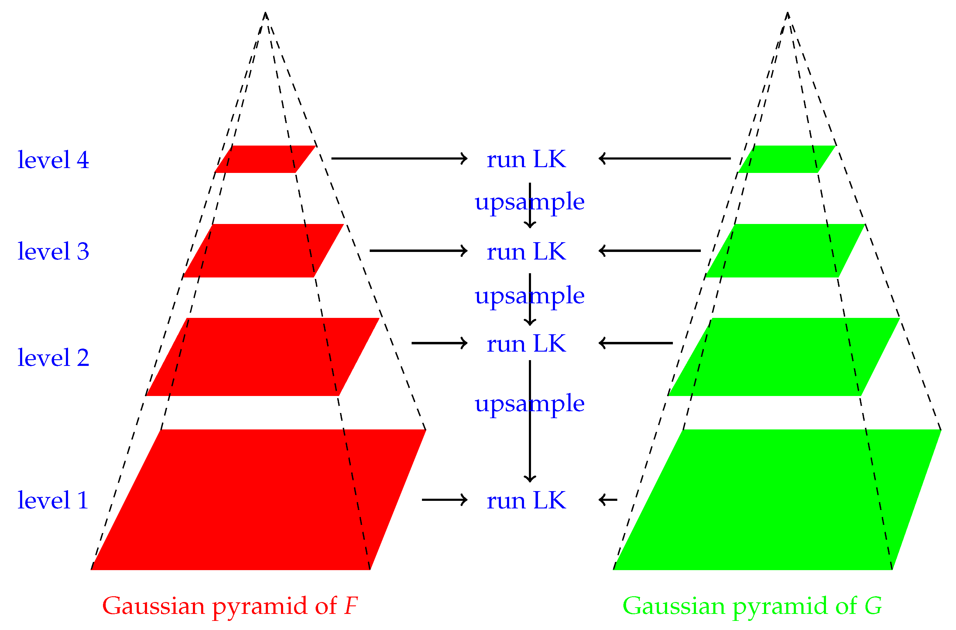
The pyramidal implementation is shown in Figure 1 for two images F and G that are taken at times t and respectively. The optical flow is computed at the top of the pyramid, level 4 (the coarsest image) in Figure 1, which is the initial condition for the computation of the optical flow at level 3 of the pyramid. It follows from (8) that (5) yields good estimates of u and v if the translation between the images at times t and is small. Only the increments between successive levels of the pyramid are therefore calculated, after warping the two images based on the flow field estimate from the coarse level. This operation yields two matrices, one for each component of the optical flow, and each matrix is upsampled to yield matrices of twice the number of rows and columns, and then passed through a modified form of the filter (9),
This process is continued to the base of the pyramid, level 1, and the optical flow at this level is the desired optical flow.
The difference in the scale factors for the filters for downsampling the images and upsampling the optical flow field arises because all the pixels in the images that are downsampled are included in the computation, but rows and columns of zeros are added to the matrices that store the components u and v before they are upsampled, such that a matrix of order is increased to a matrix of order . The computation of all the pixel values in these larger matrices cannot include the added rows and columns of zeros and thus only one quarter of the pixels in the matrices of order are included in the computation.
The matrices of the components of the optical flow must be upsampled by the filter (10) and then multiplied by two in order to preserve the values of its components between successive levels of the pyramid. In particular, two adjacent pixels have unit separation before upsampling, but their separation increases to two after upsampling. The preservation of the values of the components of the optical flow in the upsampled images therefore requires that they be multiplied by two.
The discussion above shows that the pyramidal form of the method requires that the problem be solved many times at each level of the pyramid, and thus the error in its solution must be considered. This issue is addressed in Section 3 and it is shown in Section 4 that this error is closely related to the value of the angle between b and its component that lies in the column space of A. The computed optical flow must be numerically stable and it is therefore necessary to consider its numerical condition. This issue is addressed in Section 5, and linear and non-linear condition numbers are considered.
3. The Error in the Solution of the Problem
This section considers the error e in the solution of the problem (7),
where the singular value decomposition of A is , U and V are orthogonal matrices of orders m and n respectively,
the singular values satisfy , and
The matrix U is partitioned into two matrices and ,
and it follows from the orthogonal property of U that
and
It follows from (12) that c can be written as
where and are the components of b that lie in, respectively, the spaces spanned by the columns of and . It follows from (11) that
where
and thus the error in is a measure of the proportion of b that lies in the space that is orthogonal to , and a large value of leads to a large error in . The significance of is considered in Section 4 and it is shown that it allows a geometric interpretation of the conditions that define the minimum and maximum values of e.
4. The Angle between and
It is shown in this section that , where is defined in (16), is the angle between b and its component that lies in the column space of A. This interpretation follows from the decomposition of b into a component and a component ,
Since and , there exist vectors and such that
because the columns of and form orthonormal bases for and , respectively, and thus
It follows from (13) that premultiplication of this equation by and then yields
where the first and second terms on the right are, respectively, the orthogonal projections of b onto and . It follows from (13) that the second term is orthogonal to the first term, which confirms that is orthogonal to . Also, it follows from (14) that
where
and thus is equal to the ratio of the magnitude of the orthogonal projection of b onto to the magnitude of b. Equation (15) shows that there is a simple relationship between the error in , and the angle between b and its component that lies in . The limiting cases are:
- : It follows that and , and thus .
- : It follows that and , and thus .
The ratio provides a geometric interpretation of the error in the solution of the problem, and it is shown in Section 5 that also arises in the expressions for the condition numbers of .
5. The Numerical Condition of the Optical Flow
This section considers the numerical condition of the optical flow , the solution of the problem. The condition number of A, , where , is frequently used as a measure of the stability of , but it requires qualification:
- The condition number is a function of A and it is independent of b, but is a function of A and b. This independence of b follows because is the upper bound of the ratio of the relative error in to the relative error in b with respect to all vectors and perturbations . The vector b is specified in a given problem and thus a better measure of the stability of is an upper bound of the ratio of the relative error in to the relative error in b with respect to all perturbations , for the given vector b. The condition number may therefore overestimate the true value of by many orders of magnitude if .
- The property is not, in general, satisfied in the method and thus a measure of the stability of with respect to perturbations in b that is appropriate when must be developed.
Although these points show that as a measure of the stability of has disadvantages, it has been used to assess the computational reliability of ([§II.A] [14]), ([§4.3.2] [16]), ([§2] [10]). These disadvantages of are overcome by the effective condition number of , which is a function of A and b, and therefore a more accurate measure of the stability of . This condition number is considered in Section 5.1.
The effective condition number is a linear condition number because it is assumed that the entries of A (the spatial derivatives of the intensity) are not subject to error, and only errors in b (the temporal derivatives of the intensity) are subject to error. A more realistic condition number of the optical flow requires that errors in the spatial and temporal derivatives of the intensity be considered. This inclusion leads to a non-linear extension of the effective condition number, and it is considered in Section 5.2.
5.1. The Effective Condition Number
This section considers the effective condition number of the solution of the problem, which must be solved many times in the method. It is assumed for generality that the coefficient matrix A is of order where , rather than .
The relative errors of and b are, respectively,
and the effective condition number of is defined as the maximum value of the ratio of to for the given vector b, with respect to all perturbations in b,
Theorem 1.
Proof.
The condition that must be satisfied for to be a measure of the stability of follows from (20) because if and only if . This condition is necessarily satisfied by all vectors b if A is square, but by some vectors b, not all vectors b, if . If , then and thus , and (20) yields
This leads to the definition of the condition number of , , as the upper bound of the ratio of the relative error of to the relative error of b if and only if ,
Furthermore, it follows from (12) and (19) that
and thus is the maximum value of with respect to all vectors .
The superiority of the effective condition number with respect to the condition number as a measure of the stability of follows because is a function of A and b, but is a function of A only. The example of regression in ([§3] [23]) shows the difference between these condition numbers. The dependence of on A and b is clearly advantageous, but must be used with care because it follows from (18) that the denominator contains the term . It therefore follows that is ill conditioned if is ill conditioned, and it is well conditioned if is well conditioned. It is shown in ([§4] [24]) that , and therefore , are ill conditioned if the discrete Picard condition is satisfied ([§4.5] [25]). This condition states that if the constants decay to zero faster than the singular values decay to zero, that is,
then is ill conditioned. This condition can be derived from ,
where is the ith column of V. If b is perturbed to , then is perturbed to
and there exists a constant s such that the perturbations , satisfy
These inequalities follow because the perturbations are approximately constant but the coefficients decay to zero because the discrete Picard condition (21) is satisfied, and thus from (23),
Since the discrete Picard condition is satisfied, can be approximated with a small error by only considering the first s singular values in (22),
and thus
It follows that
and thus the norm of the perturbation is approximately proportional to the magnitude of the noise and inversely proportional to the smallest singular value of A, from which it follows that is ill conditioned if the discrete Picard condition (21) is satisfied. It is seen that is ill conditioned if it is dominated by the large singular values of A, in which case is dominated by the small singular values of A.
The satisfaction of the discrete Picard condition is necessary for the application of Tikhonov regularisation because it guarantees that the regularisation error is small and the regularised form of is numerically stable ([§5] [23]). Tikhonov regularisation is used for the removal of blur from images because experiments have shown that many images satisfy the discrete Picard condition [26]. This condition forms the prior information that guarantees that Tikhonov regularisation is effective for image deblurring, and more generally, the ill conditioned property of limits its practical use if prior information is not available. The condition number is, however, an important condition measure because, as shown above, it defines the conditions between A and b for which is well conditioned, and the conditions for which is ill conditioned.
It has been shown that is ill conditioned if is ill conditioned, but its upper bound is numerically stable, and an expression for this bound is developed in Theorem 2. This bound includes the term that is defined in (16), and thus the error in the solution of the problem is related to the numerical condition of .
Theorem 2.
Proof.
Equation (24) shows that the condition number of increases rapidly as . For example, if a window of order is used, then and the error in is equal to zero if and only if b lies in the two dimensional subspace spanned by the columns of A, in the space , and the error in is due to the component of b that lies in the space that is orthogonal to . The condition number of is large if , even if .
Example 1.
Consider the matrix A and vector b,
The singular values of A are and , and thus . It may therefore be thought that the solution of the problem is well conditioned but this is incorrect because b is orthogonal to ,
It follows that and .
The left singular matrix U of , and the matrices and are
and thus
which confirm that b is orthogonal to .
5.2. A Non-Linear Condition Number
This section extends the linear effective condition number considered in Section 5.1 by including perturbations in the coefficient matrix A, such that the perturbed solution of the problem is
An expression for the condition number of when A and b are perturbed is developed in Theorem 3.
Theorem 3.
The condition number of when A and b are perturbed by, respectively, and such that
is
Proof.
The pseudo-inverse of is
where, to first order,
and thus
to first order. It therefore follows from (25) that
and thus
An upper bound for the last term in (27) allows to be expressed in terms of and . In particular,
and thus (27) becomes
and thus the inclusion of errors in the spatial derivatives of the intensity is significant because of the term .
It was stated in Section 5.1 that the effective condition number is ill conditioned if the discrete Picard condition is satisfied, in which case (27) and its upper bound (28) cannot be computed reliably. This problem is addressed by using the upper bound (24) for the value of in (28). The condition number (27) is, however, useful because it shows that the inclusion of perturbations in the spatial derivatives of the intensity causes a significant increase in the condition number of the optical flow.
6. Examples
This section contains two examples that show the errors and condition numbers of the optical flow at each level of the pyramid. The Middlebury data set [1] is used in Examples 2 and 3, and the following numerical measures are considered:
- The condition number , the upper bound of the effective condition number, , and the non-linear condition number .
- The angle between b and its component that lies in .
- The error e in the solution of the problem.
Example 2.
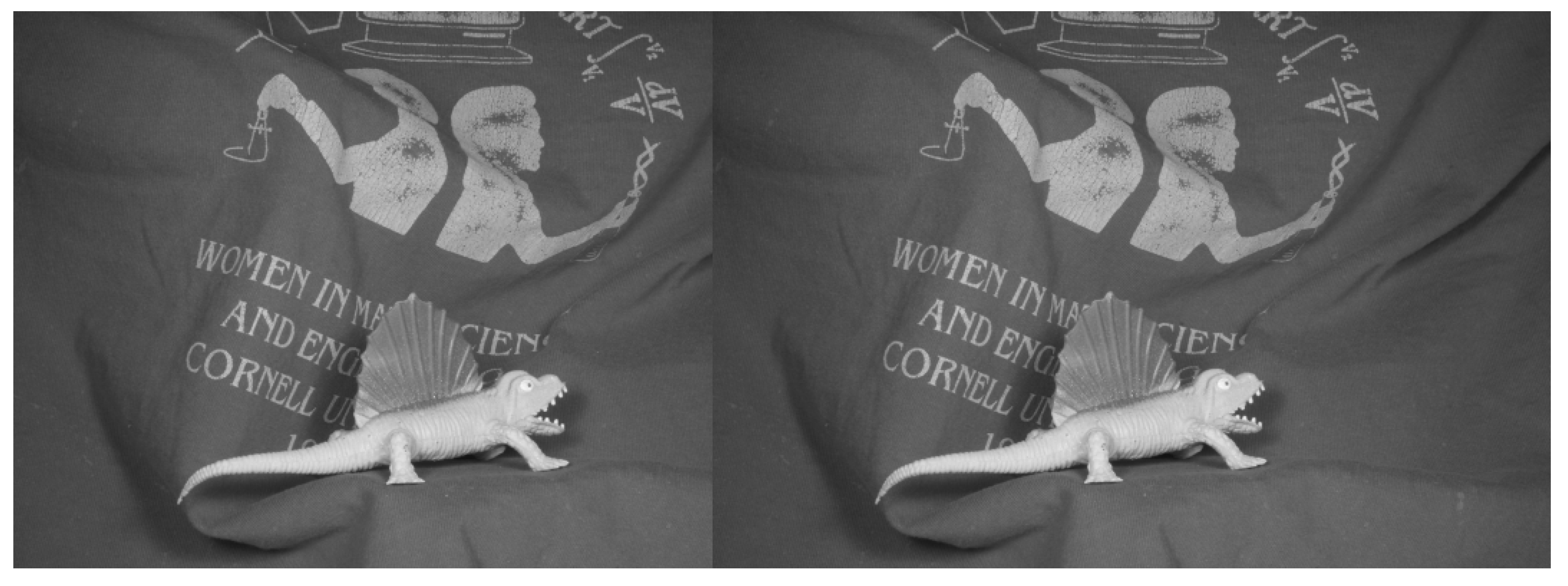
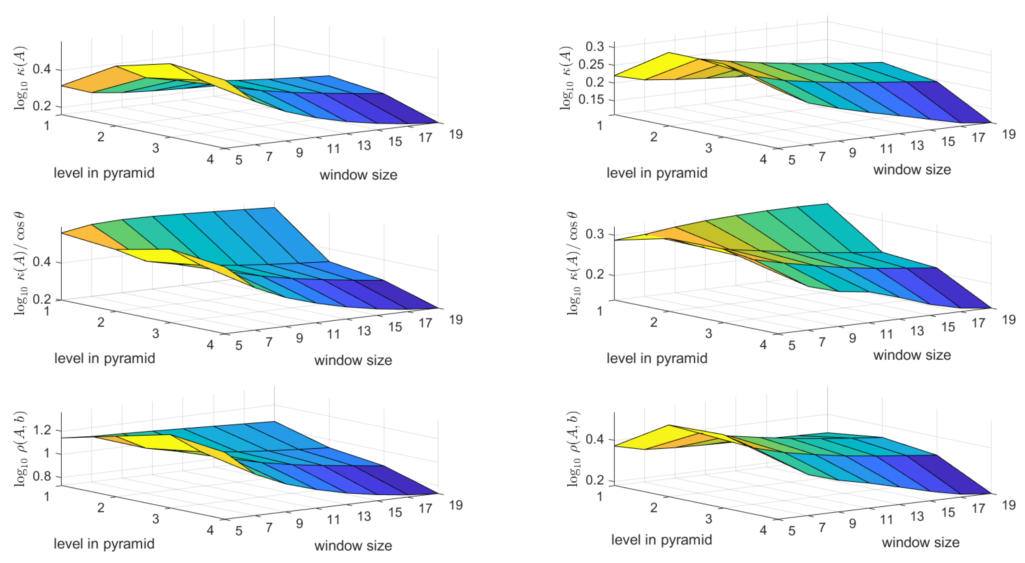
The five measures listed above (the three condition numbers, the angle θ and the error e in ) were computed in each window for windows of side lengths , at each level of a pyramid that has four levels, for the images in Figure 2. The mean and standard deviation of , the upper bound of the effective condition number, and the non-linear condition number , at each level of the pyramid and for each window size, are shown in Figure 3. The figures in the left column show that, as expected, the mean of at each of the 32 points in the grid is larger than the corresponding values of and . Also, the means of and increase, but not monotonically, as the pyramid is descended from the coarsest image (level 4) to the finest image (level 1), and they decrease as the window size increases, at each level of the pyramid. The variation of the mean of each condition number, Figure 3 (left), is similar to the variation of its standard deviation, Figure 3 (right).
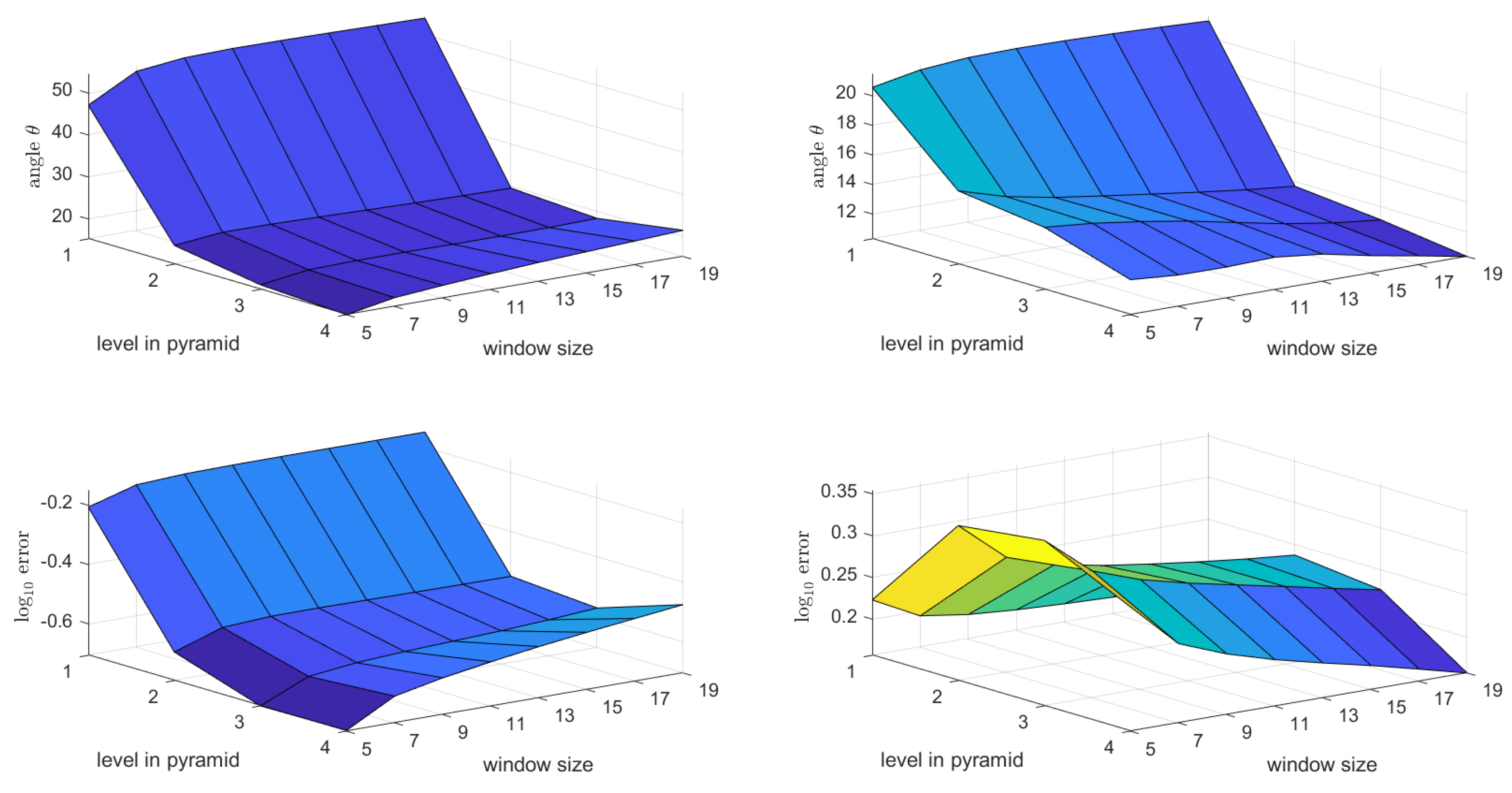
The mean and standard deviation of the angle θ, where is defined in (16), and the error , where e is defined in (11), are shown in Figure 4. It is seen that the mean of θ is approximately constant for windows of side length 7 pixels or more at levels 2, 3 and 4 of the pyramid. Figure 4 (left) shows that the variation of the means of θ and are very similar, but Figure 4 (right) show that, for each measure, the standard deviation is significant, which implies that there is considerable variation of each measure.
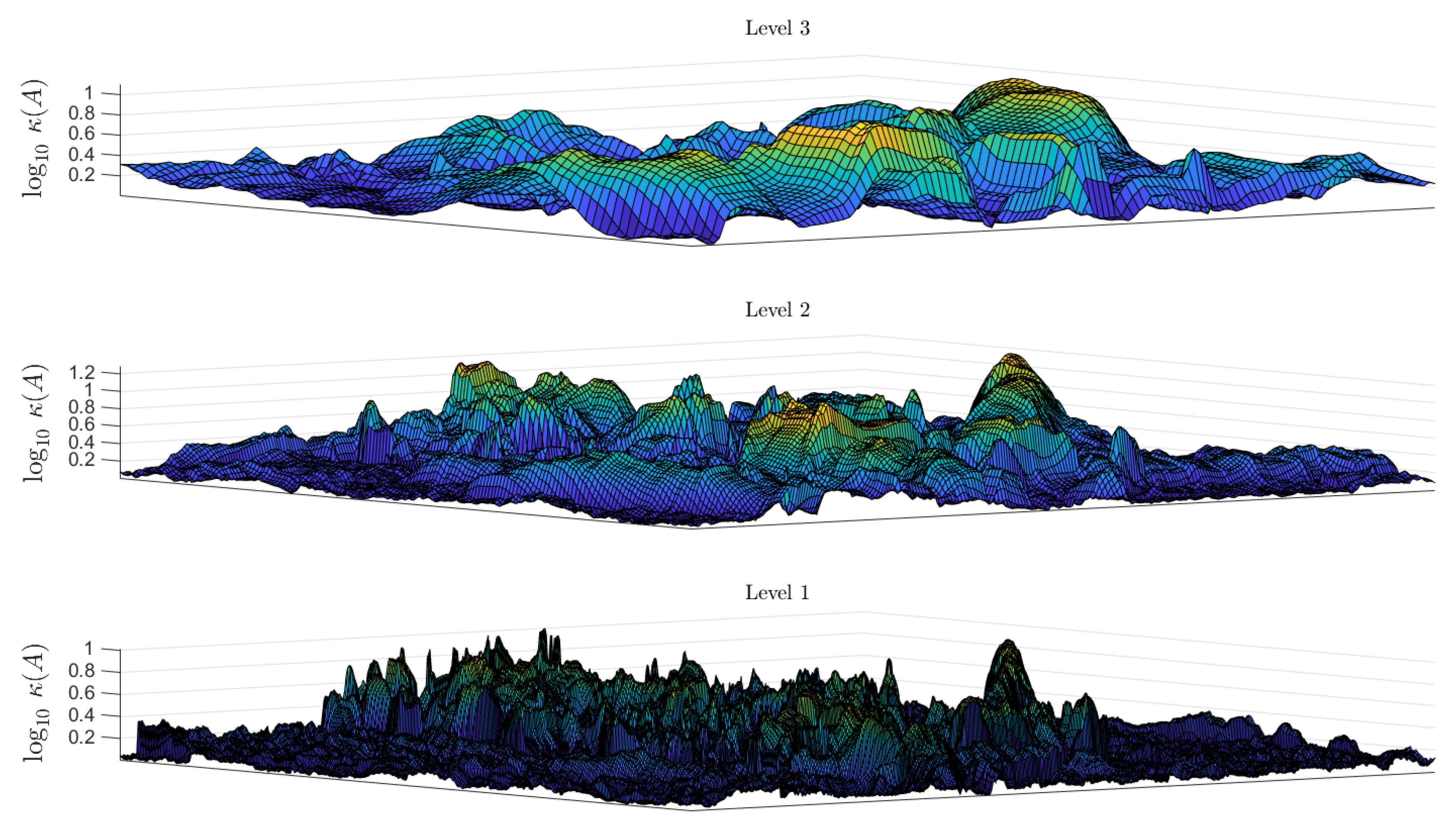
Example 3.
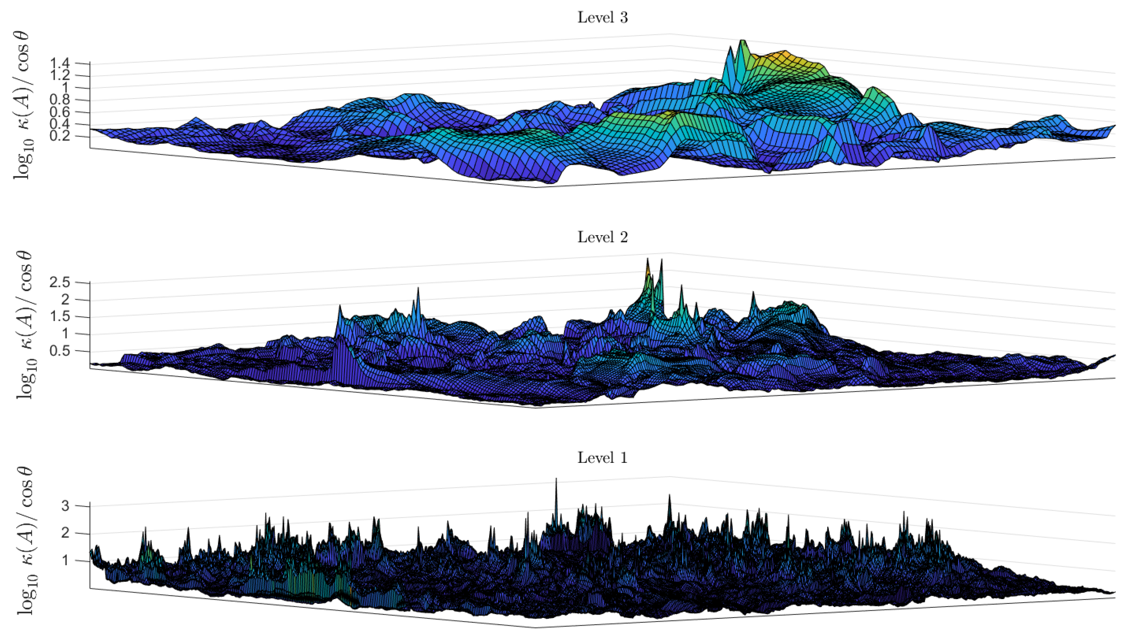
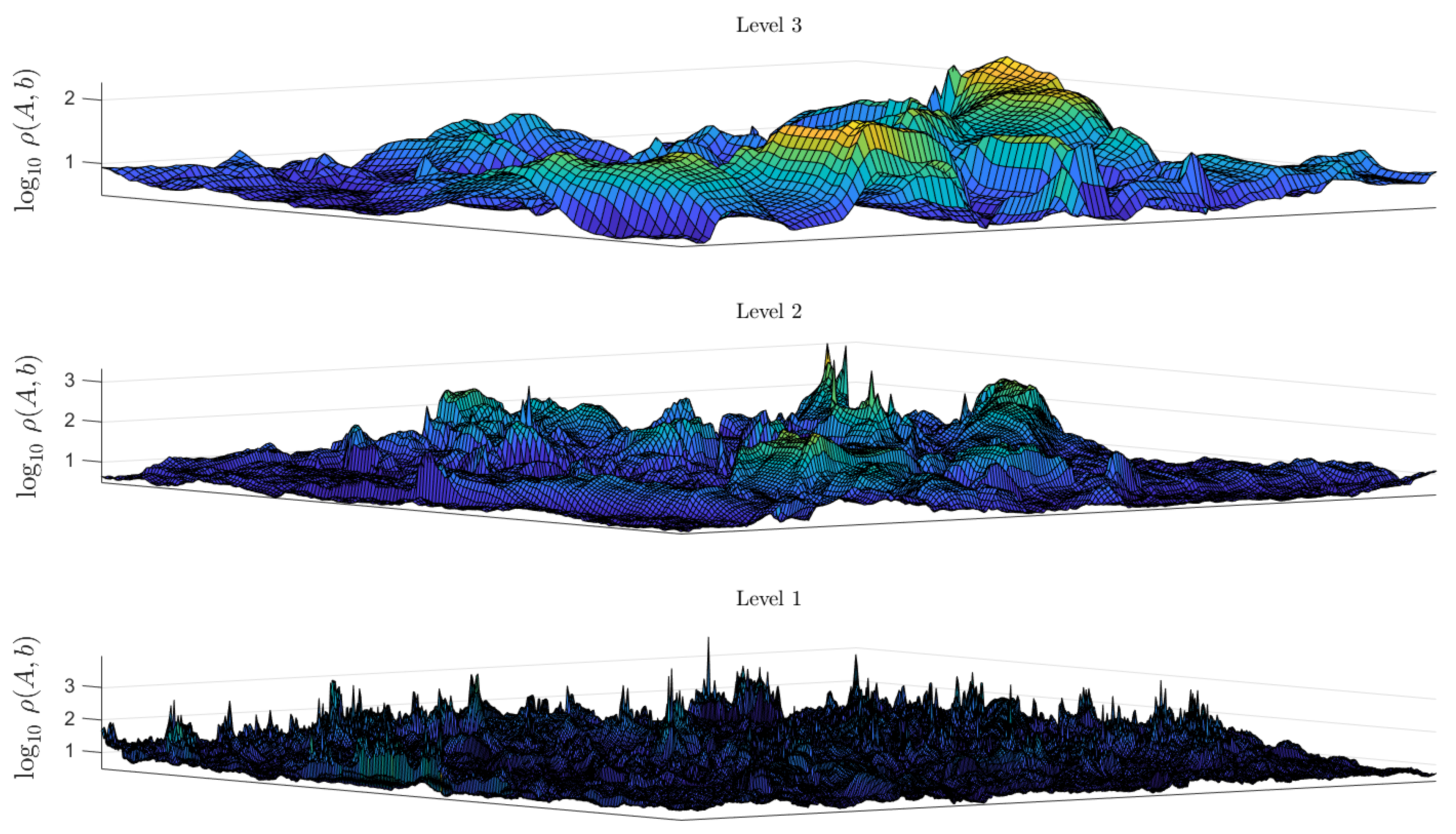
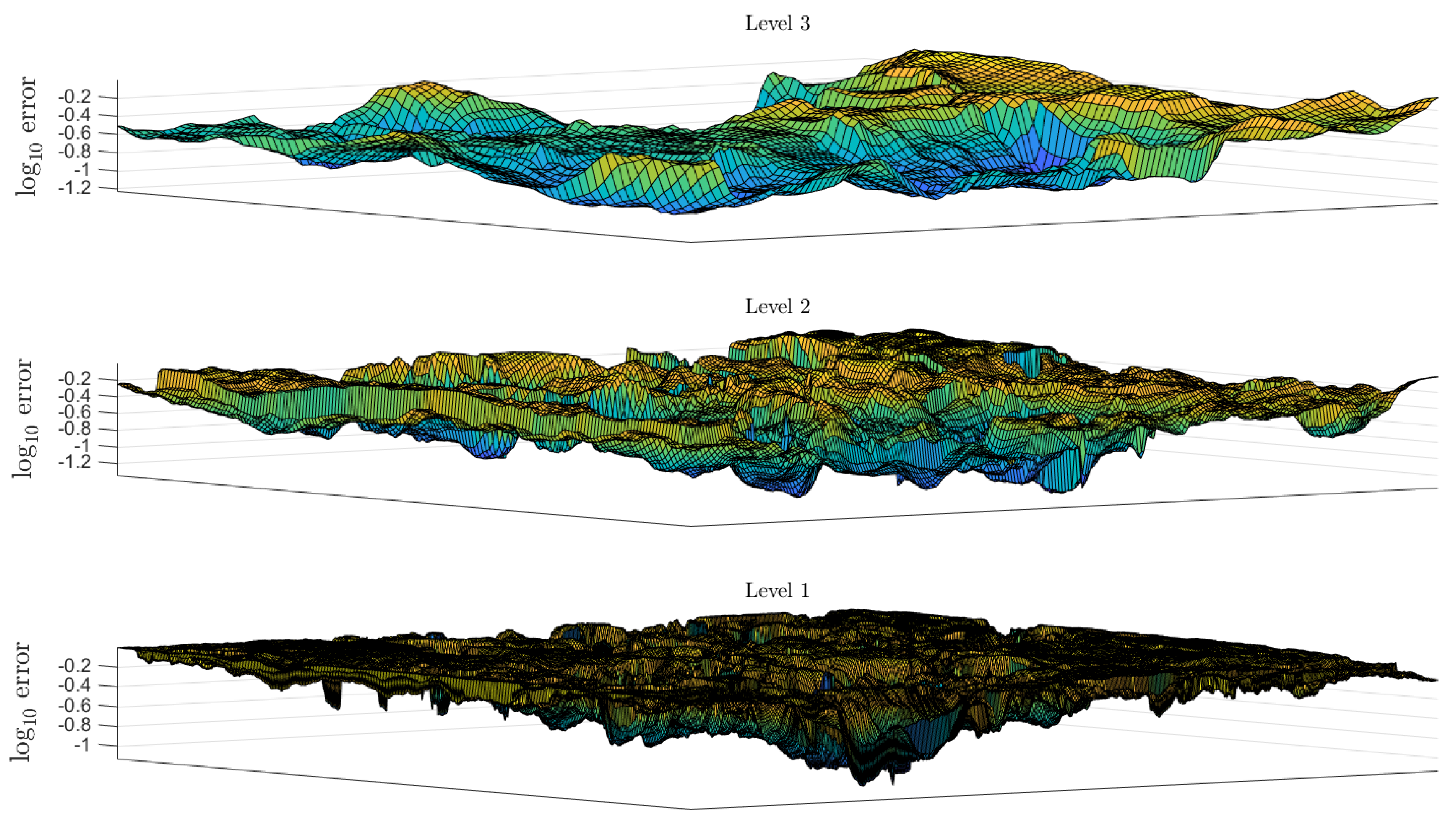
The method with a pyramid of three levels was applied to the images in Figure 2, with a window of size . The condition number , upper bound of the effective condition number, the non-linear condition number , angle θ and error were computed for every problem in the windows for each level of the pyramid. Figure 5 shows the axes and size of the image at each level of the pyramid for Figure 6, Figure 7, Figure 8, Figure 9 and Figure 10. These figures show that the quantities above increase, and the standard deviation of each of these quantities increases, as the pyramid is descended. The figures are therefore consistent with Figure 3 and Figure 4, and it follows that the computational reliability of the optical flow decreases as the pyramid is descended.
Figure 9 shows that the values of the local maxima of the angle θ increase significantly as the pyramid is descended. In particular there are many problems for which θ is about 80 degrees, from which it follows that the errors in the solutions of these problems are large. This result is consistent with the plots of the condition numbers in Figure 7 and Figure 8. Furthermore, it follows from (15) that large values of θ are associated with large errors e, which is confirmed in Figure 10.
7. Summary and Conclusions
The work in this paper considers the numerical properties of the solution of the problem because of their consequences on the computed optical flow. These consequences are compounded by the large number of problems that must be solved in the method, where the solutions of the problems at level l of the pyramid form the data, after upsampling, for the problems at level of the pyramid. It has been shown that the large values of the condition numbers and , and error e, of the solution of the problem arise because a significant component of b lies in the space that is orthogonal to , and thus the terms and in, respectively, the expressions for the condition numbers and error are significant. It has been shown that the error and condition numbers of the problem increase as the pyramid is descended from the top level (coarsest image) to the bottom level (finest image) and thus the fidelity of the computed optical flow decreases as the pyramid is descended. There have been several studies that consider the errors associated with the method, but the new aspect of the work described in this paper is the extensive use of computational linear algebra, specifically, condition estimation and error analysis of the solution of the problem.
The large values of the condition numbers and errors follow from the assumption that the optical flow in each window at each level of the pyramid is constant, that is, the motion in each window can be represented by a translation. It follows that an improved form of the method requires that a richer class of motions be allowed in each window, and this is achieved by the introduction of warping functions in the method [17]. These warping functions are defined by parametric models, for example, affine and projective models, and the values of the parameters of these models are computed in the optimisation procedure in an extended form of the method.
Funding
This research received no external funding.
Data Availability Statement
The data used in this paper are taken from the Middlebury data set [1], which is in the public domain and frequently used in computer vision.
Conflicts of Interest
The author declares that he does have not relationships or interests that have direct or potential influence, or impart bias, on the work.
References
- Baker, S.; Scharstein, D.; Lewis, J.; Roth, S.; Black, M.; Szeliski, R. A database and evaluation methodology for optical flow. Int. J. Computer Vision 2011, 92, 1–31. [Google Scholar] [CrossRef]
- Horn, B.; Schunck, B. Determining optical flow. Artif. Intell. 1981, 17, 185–203. [Google Scholar] [CrossRef]
- Lucas, B.D.; Kanade, T. An iterative image registration technique with an application to stereo vision. In Proceedings of the 7th International Joint Conference on Artificial Intelligence, Vancouver, BC, Canada, 24–28 August 1981; pp. 674–679. [Google Scholar]
- Fortun, D.; Bouthemy, P.; Kervrann, C. Optical flow modeling and computation: A survey. Comput. Vis. Image Underst. 2015, 134, 1–21. [Google Scholar] [CrossRef]
- Hofinger, M.; Bulò, S.; Porzi, L.; Knapitsch, A.; Pock, T.; Kontschieder, P. Improving optical flow on a pyramidal level. In Proceedings of the European Conference on Computer Vision, Glasgow, UK, 23–28 August 2020; pp. 770–786. [Google Scholar]
- Shah, S.T.H.; Xuezhi, X. Traditional and modern strategies for optical flow: An investigation. SN Appl. Sci. 2021, 3. [Google Scholar] [CrossRef]
- Tu, Z.; Xie, W.; Zhang, D.; Poppe, R.; Veltkamp, R.; Li, B.; Yuan, J. A survey of variational and CNN-based optical flow techniques. Signal Process. Image Commun. 2019, 72, 9–24. [Google Scholar] [CrossRef]
- Zhai, M.; Xiang, X.; Lv, N.; Kong, X. Optical flow and scene flow estimation: A survey. Pattern Recognit. 2021, 114, 107861. [Google Scholar] [CrossRef]
- Savian, S.; Elahi, M.; Tillo, T. Optical flow estimation with deep learning: A survey on recent advances. In Deep Biometrics; Jiang, R., Li, C.T., Crookes, D., Meng, W., Rosenberger, C., Eds.; Springer: Berlin/Heidelberg, Germany, 2020; pp. 257–287. [Google Scholar]
- Lin, T.; Barron, J. Image reconstruction error for optical flow. Res. Comput. Robot. Vis. 1995, 269–290. [Google Scholar]
- Kearney, J.; Thompson, W.; Boley, D. Optical flow estimation: An error analysis of gradient-based methods with local optimization. IEEE Trans. Pattern Anal. Mach. Intell. 1987, 9, 229–244. [Google Scholar] [CrossRef]
- Golub, G.H.; Loan, C.F.V. Matrix Computations; John Hopkins University Press: Baltimore, MD, USA, 2013. [Google Scholar]
- Tsai, C.; Galatsanos, N.; Katsaggelos, A. Total least squares estimation of stereo optical flow. In Proceedings of the IEEE International Conference on Image Processing, Chicago, IL, USA, 4–7 October 1998; pp. 622–626. [Google Scholar]
- Kim, Y.; Kak, A. Error analysis of robust optical flow estimation by least median of squares methods for the varying illumination model. IEEE Trans. Pattern Anal. Mach. Intell. 2006, 28, 1418–1435. [Google Scholar] [CrossRef]
- Tarasenko, V.; Park, D. Detection and tracking over image pyramids using Lucas and Kanade algorithm. Int. J. Appl. Eng. Res. 2016, 11, 6117–6120. [Google Scholar]
- Klette, R. Concise Computer Vision: An Introduction into Theory and Applications; Springer: London, UK, 2014. [Google Scholar]
- Baker, S.; Matthews, I. Lucas-Kanade 20 years on: A unifying framework. Int. J. Computer Vision 2004, 56, 221–255. [Google Scholar] [CrossRef]
- Brandt, J.W. Analysis of bias in gradient-based optical flow estimation. In Proceedings of the 28th Asilomar Conference of Signals, Systems and Computers, Pacific Grove, CA, USA, 31 October–2 November 1994; pp. 721–725. [Google Scholar]
- Pham, T.Q.; Bezuijen, M.; van Vliet, L.J.; Schutte, K.; Hendriks, C.L.L. Performance of optimal registration estimators. Proc. SPIE 2005, 5817, 133–144. [Google Scholar]
- Robinson, D.; Milanfar, P. Fundamental performance limits in image registration. IEEE Trans. Image Process. 2004, 13, 1185–1199. [Google Scholar] [CrossRef] [PubMed]
- Burt, P. Fast filter transforms for image processing. Comput. Graph. Image Process. 1981, 16, 20–51. [Google Scholar] [CrossRef]
- Burt, P.; Adelson, E. The Laplacian pyramid as a compact image code. IEEE Trans. Comm. 1983, 31, 532–540. [Google Scholar] [CrossRef]
- Winkler, J.R.; Mitrouli, M. Condition estimation for regression and feature estimation. J. Comput. Appl. Math. 2020, 373, 112212. [Google Scholar] [CrossRef]
- Winkler, J.R.; Mitrouli, M.; Koukouvinos, C. The application of regularisation to variable selection in statistical modelling. J. Comput. Appl. Math. 2022, 404, 113884. [Google Scholar] [CrossRef]
- Hansen, P.C. Rank-Deficient and Discrete Ill-Posed Problems: Numerical Aspects of Linear Inversion; SIAM: Philadelphia, PA, USA, 1998. [Google Scholar]
- Hansen, P.C.; Nagy, J.G.; O’Leary, D.P. Deblurring Images: Matrices, Spectra, and Filtering; SIAM: Philadelphia, PA, USA, 2006. [Google Scholar]
Figure 1.
The pyramid implementation of the Lucas-Kanade method.

Figure 2.
The images used in Examples 2 and 3.

Figure 3.
The variation of the mean (left) and standard deviation (right) of the condition number , upper bound of the effective condition number, and the non-linear condition number with the size of the window and number of levels in the pyramid, for Example 2.
Figure 3.
The variation of the mean (left) and standard deviation (right) of the condition number , upper bound of the effective condition number, and the non-linear condition number with the size of the window and number of levels in the pyramid, for Example 2.

Figure 4.
The variation of the mean (left) and standard deviation (right) of the angle and the error , with the size of the window and number of levels in the pyramid, for Example 2.
Figure 4.
The variation of the mean (left) and standard deviation (right) of the angle and the error , with the size of the window and number of levels in the pyramid, for Example 2.

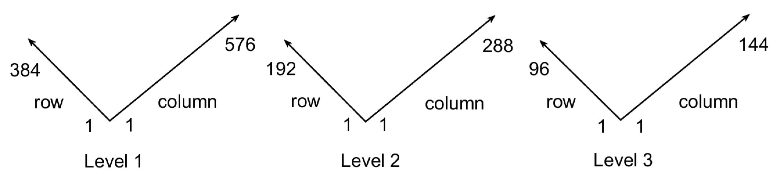
Figure 5.
The sizes of the images at level 1 (), level 2 () and level 3 () in Figure 6, Figure 7, Figure 8, Figure 9 and Figure 10, for Example 3.

Figure 6.
The condition number at level three (top), level two (middle) and level one (base) of the pyramid, for Example 3.
Figure 6.
The condition number at level three (top), level two (middle) and level one (base) of the pyramid, for Example 3.

Figure 7.
The upper bound of the effective condition number at level three (top), level two (middle) and level one (base) of the pyramid, for Example 3.
Figure 7.
The upper bound of the effective condition number at level three (top), level two (middle) and level one (base) of the pyramid, for Example 3.

Figure 8.
The non-linear condition number at level three (top), level two (middle) and level one (base) of the pyramid, for Example 3.
Figure 8.
The non-linear condition number at level three (top), level two (middle) and level one (base) of the pyramid, for Example 3.

Figure 9.
The angle at level three (top), level two (middle) and level one (base) of the pyramid, for Example 3.
Figure 9.
The angle at level three (top), level two (middle) and level one (base) of the pyramid, for Example 3.

Figure 10.
The error at level three (top), level two (middle) and level one (base) of the pyramid, for Example 3.
Figure 10.
The error at level three (top), level two (middle) and level one (base) of the pyramid, for Example 3.

Disclaimer/Publisher’s Note: The statements, opinions and data contained in all publications are solely those of the individual author(s) and contributor(s) and not of MDPI and/or the editor(s). MDPI and/or the editor(s) disclaim responsibility for any injury to people or property resulting from any ideas, methods, instructions or products referred to in the content. |
© 2024 by the author. Licensee MDPI, Basel, Switzerland. This article is an open access article distributed under the terms and conditions of the Creative Commons Attribution (CC BY) license (https://creativecommons.org/licenses/by/4.0/).
Share and Cite
MDPI and ACS Style
Winkler, J.R. Error Analysis and Condition Estimation of the Pyramidal Form of the Lucas-Kanade Method in Optical Flow. Electronics 2024, 13, 812. https://doi.org/10.3390/electronics13050812
AMA Style
Winkler JR. Error Analysis and Condition Estimation of the Pyramidal Form of the Lucas-Kanade Method in Optical Flow. Electronics. 2024; 13(5):812. https://doi.org/10.3390/electronics13050812
Chicago/Turabian StyleWinkler, Joab R. 2024. "Error Analysis and Condition Estimation of the Pyramidal Form of the Lucas-Kanade Method in Optical Flow" Electronics 13, no. 5: 812. https://doi.org/10.3390/electronics13050812
Note that from the first issue of 2016, this journal uses article numbers instead of page numbers. See further details here.