
A Fast Phase-Only Beamforming Algorithm for FDA-MIMO Radar via Kronecker Decomposition

1
School of Air Defense and Antimissile, Air Force Engineering University, Xi’an 710051, China
2
College of Information and Communication, National University of Defense Technology, Wuhan 430010, China
*
Author to whom correspondence should be addressed.
Electronics 2024, 13(2), 337; https://doi.org/10.3390/electronics13020337
Submission received: 14 December 2023
/
Revised: 9 January 2024
/
Accepted: 11 January 2024
/
Published: 12 January 2024
(This article belongs to the Special Issue Artificial Intelligence (AI) Based Radar Signal Processing and Radar Imaging)
Abstract
:This paper proposes a fast phase-only beamforming algorithm for frequency diverse array multiple-input multiple-output radar systems. Specifically, we use the Kronecker decomposition to decompose the desired phase-only weight vector into phase-only transmit and receive weight vectors and to decompose the target steering vector into transmit and receive steering vectors. By using the properties of the Kronecker product, the transmit and receive steering vectors and the transmit and receive weight vectors with the Vandermonde structure are decomposed into Kronecker factors with uni-modulus vectors, respectively. On this basis, in order to maintain the mainlobe gain and form a deep null at the desired position, the Kronecker factors are divided into two parts.The first component, referred to as the interference suppression factors, is responsible for creating deep nulls. The second component, known as the signal enhancement factor, maintains the mainlobe gain. We provide an analytical solution with low complexity for the Kronecker factors. This strategy can obtain the phase-only weights while effectively forming a deep null at the desired position. Numerical experiments are conducted to verify the effectiveness of the proposed algorithm.
1. Introduction
Antenna arrays play a crucial role in various industries of modern information technology, including radar, communications, remote sensing, etc. [1,2,3,4,5,6]. Beamforming, as a fundamental technique in array signal processing, is widely employed to enhance target signal and suppress interference by creating deep nulls in undesired directions. Improving the interference suppression capability of antenna arrays is a critical requirement for radar and communication systems.
Over the past few decades, numerous beamforming techniques have been investigated [7,8,9,10,11,12,13]. Conventional beamforming techniques require adjusting the amplitude and phase of the receive filter, resulting in higher hardware costs at the receiver. Therefore, previous works have explored phase-only beamforming techniques for phased array radar [10,11,12,13], which utilize neural networks [10], numerical optimization [11], and other methods [12,13] to obtain phase-only weights. However, these techniques may be limited by computational complexity. In order to reduce computational complexity and improve practicality, a phase-only array response adjustment via the geometric approach was proposed [14]. Unfortunately, this method [14] can only rapidly adjust the response at a single point and cannot simultaneously form deep nulls for multiple points. Moreover, it is worth noting that these techniques [7,8,9,10,11,12,13,14] primarily aim to create deep nulls in desired directions, but they are limited in their ability to create deep nulls at specific locations due to the angle-dependent beam pattern of phased array radar systems. From a practical point of view, it is possible to encounter interference signals that have similar angles as the target of interest [15,16]. As a result, there is a demand to investigate beamforming techniques that can effectively form deep nulls at specific locations.
Recently, the frequency diverse array (FDA) radar has gained significant attention from academia due to its degrees of freedom (DOFs) in the range domain [17,18,19]. In contrast to the capability of forming nulls in a specific direction in the beam pattern of phased array radar, by introducing frequency offsets between the elements of the transmitter, FDA allows for the control of nulls in both range and angle dimensions, thus effectively suppressing interference signals from specific directions and ranges. However, the beam pattern of the FDA radar exhibits time-varying characteristics, necessitating the integration of Multiple-Input Multiple-Output (MIMO) technology at the receiver end to achieve an equivalent time-invariant beam pattern [20,21,22], thereby fully leveraging the advantages of the two-dimensional (2D) range-angle beam pattern of the FDA radar.
Based on this capability, numerous beamforming techniques [23,24,25,26,27] have been proposed. For instance, Lan et al. [26] proposed two iterative algorithms with multi-response control based on the oblique projection (MRCOP) method, namely the concurrent MRCOP (C-MRCOP) and the successive MRCOP (S-MRCOP). Moreover, two approaches, namely point-by-point successive null broadening control (SNBC) and multi-point concurrent null broadening control (CNBC), were developed for suppressing interference [27]. These approaches [27] were designed to broaden nulls at specific positions and effectively mitigate interference signals. Apart from the aforementioned works, there are various other beamforming techniques for the FDA-MIMO radar, such as transmit beam space design [28], cognitive FDA-MIMO radar beamforming [29], low probability of intercept of FDA-MIMO radar beamforming [30], and so on [31,32,33]. It is worth noting that none of the aforementioned methods investigate the phase-only beamforming technique for the FDA-MIMO radar. This implies that the mentioned approaches are not capable of utilizing phase shifters at the receiver to form deep nulls at desired positions. Thus, the implementation of these methods requires a complex and high-cost hardware architecture. For the FDA-MIMO radar, two data-independent phase-only beamforming methods were proposed using the convex optimization technique [34]. However, these methods still have computational complexities, and cannot find an efficient solution in polynomial time when the number of antennas is large. To the best of our knowledge, there have been limited reports on the fast phase-only beamforming technique for the FDA-MIMO radar.
Motivated by this research gap, we propose a fast phase-only beamforming method via the Kronecker decomposition [35] for the FDA-MIMO radar. In our work, we utilize the Kronecker decomposition to decompose the desired phase-only weight vectors into phase-only transmit and receive weight vectors, and decompose the target steering vector into transmit and receive steering vectors. The steering vectors and weight vectors of the transmit and receive modes with the Vandermonde structure are then decomposed into Kronecker factors with uni-modulus vectors, respectively. Subsequently, we divide the Kronecker factors into two parts to achieve interference suppression and signal enhancement. Our algorithm can rapidly form a deep null at the desired position with low computational complexities. Numerical experiment results demonstrate the effectiveness and superiority of the proposed method. We briefly summarize the research contributions of our work as follows:
- (1)
- We propose a phase-only beamforming design algorithm for the FDA-MIMO radar based on Kronecker decomposition.
- (2)
- We offer an analytical solution of the interference suppression factors and signal enhancement factors.
- (3)
- The proposed algorithm can form deep nulls at specified locations with very low complexity and reduce the hardware cost of the FDA-MIMO radar system.
The remainder of this paper is organized as follows. In Section 2, the system model is introduced, and the problem formulation is presented. Section 3 presents the analytical solution for phase-only weight by designing the interference suppression factors and signal enhancement factors. Numerical simulations are employed in Section 4 to validate the effectiveness of the proposed method. Finally, concluding remarks are provided in Section 5.
Notations: Throughout this paper, notations , and are used to represent the conjugate, transpose and conjugate transposes, respectively. denotes the modulus of complex number w. ⊗ represents the Kronecker product. is the phase of . represents the Euclidean norm of a vector. outputs the remainder after dividing by . Π denotes the cumulative product operation. refers to the orthogonal space of . represents the identity matrix, and indicates the sets of the complex matrix.
2. Signal Model and Problem Formulation
In this section, we introduce the FDA-MIMO radar signal model and the phase-only beamforming problem.
2.1. Signal Model
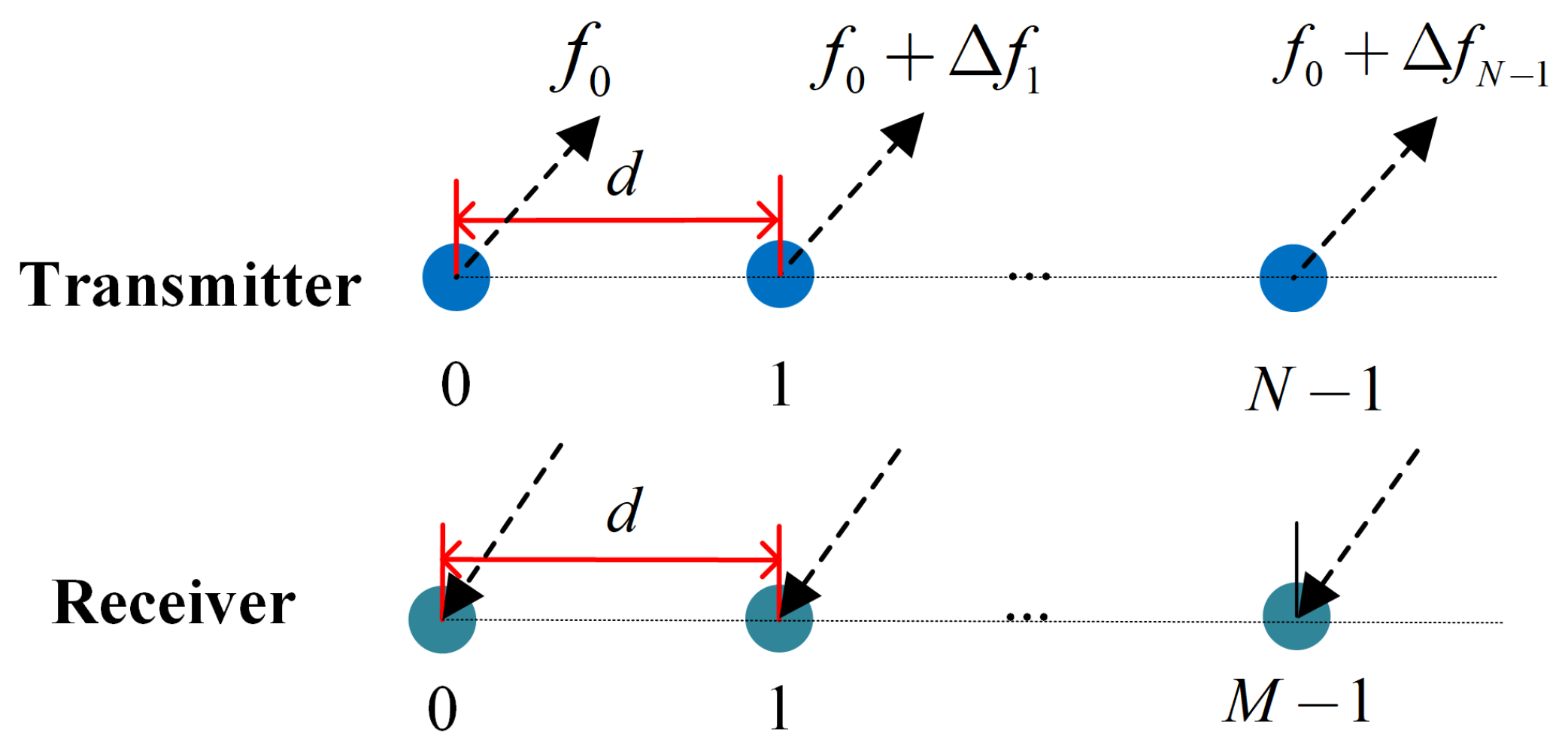
We consider a monostatic FDA-MIMO radar, as illustrated in Figure 1. Let us assume that the transmitter and receiver both adopt a Uniform Linear Arrays (ULA) consisting of N and M elements, respectively. The antenna array element spacing is set to , where represents the wavelength and is given by . c denotes the speed of light. represents the transmitting frequency of the first element of the transmitter, acting as the reference carrier frequency. Setting a linear frequency offset between the transmitting frequencies of different transmitter elements [17,18,19], the transmitting frequency of the nth element is
The transmit signal of the n-th element can be expressed as
where E is the transmitted energy, t denotes the time within the radar pulse, T is the radar pulse duration and represents the baseband envelope of the nth transmit element, i.e., , which satisfies the orthogonality condition,
where denotes the delay time, .
Assuming a far-field target located at angle and range r, after matched filtering is performed on the receive elements, the received target echo signal by the FDA-MIMO radar at time t can be expressed as follows (more details can be found in [20,21,22]):
where is the complex coefficient after matched filtering, represents the noise signal. is the array steering vector, which can be expressed as
where is the range angle-dependent transmit steering vector, defined as
and is the receive steering vector determined by the angle, given by
where and denote the transmit and receive spatial frequencies, respectively.
2.2. Problem Formulation
In order to design the phase-only weight vector to suppress the interference while ensuring the target signal gain, the weight vector needs to maximize the output signal-to-noise ratio (SINR) after beamforming. This objective function can be modeled as
where represents the signal covariance matrix, defined as
is the power of the signal, is the target steering vector. denotes the interference plus noise covariance matrix. Assuming interference and noise are independent, we can express as
where the noise is assumed to be a white Gaussian signal with zero mean and covariance matrix . and are the power of the jth interference and noise, respectively. is the jth interference steering vector.
It can be found in (11) that to maximize the output SINR, we need to maximize the numerator and minimize the denominator of (11). Then, to maximize SINR while obtaining the phase-only weight vector, the following problem can be obtained:
where constraint (12b) is used to enhance the mainlobe gain, is a small positive number in constraint (12c) to suppress interference. And constraint (12d) ensures the phase-only weight vector. Notice that Problem (12) is a nonconvex problem. In the next section, we design an analytical method to solve Problem (12) and obtain the phase-only weight vector.
3. The Phase-Only Beamforming Based on Kronecker Decomposition
In this section, we introduce a fast phase-only beamforming technique via Kronecker decomposition for the FDA-MIMO radar. For simplicity, we hypothesize that the numbers of transmitter and receiver satisfy and , where P and Q are positive integer (we discuss the general case where the number of the transmitter or receiver is an arbitrary positive integer in Section 3.4).
3.1. The Proposed Phase-Only Weight Vector Design Model
For the convenience of subsequent calculation, before designing the phase-only weight vector, we define weight vector to be a feasible solution to Problem (12) with the following form:
where and are defined as the transmit and receive weight vectors, respectively. Next, we introduce the following problem (14):
where and represent the target transmit and receive steering vectors, respectively. and are the jth interference transmit and receive steering vectors, respectively. Compared to Problem (12), in Problem (14), variable is replaced with and . Moreover, to maximize SINR, we expect the left side of (12c) to be as small as possible and set the left-hand side of Constraint (14c) equal to zero. In the next section, we present an approach based on Kronecker decomposition to design phase-only weight vectors and .
3.2. Kronecker Decomposition of Weight Vector and Steering Vector
First of all, we introduce an important lemma on Kronecker decomposition.
Lemma 1
(Kronecker Decomposition [35]). Let us consider vector whose elements have uni-modulus and which has a Vandermonde structure according to the following expression:
where Φ is fixed. Vector can be decomposed as , where with being positive integers. Each factor with a length of is given by with .
We note that if , then in Lemma 1 is now simplified as . Recalling the transmit and receive steering vectors in (6) and (7), we can observe that and exhibit a Vandermonde structure, as stated in Lemma 1. Hence, and can be decomposed as (16) and (17), respectively.
where and denote the transmit and receive Kronecker factors, respectively ( and ), which are defined as
where .
According to Problem (14), the design of and must satisfy (14b) for target echo enhancement and (14c) for interference suppression. To meet these requirements and simplify the algorithm, we assume that weight vectors and have a Vandermonde structure. Then, and are decomposed as
where and denote the pth and qth Kronecker factors of the transmit and receive weight vectors, respectively. Building upon Equations (20) and (21), the design of and is converted into the design of and . We introduce the design method of the Kronecker factors and synthesize the phase-only weight vector in the next subsection.
3.3. Design the Phase-Only Weight Vector
In the previous subsection, based on the Kronecker decomposition, the steering vector and the weight vector are decomposed into multiple Kronecker factors. In accordance with Equations (16), (17), (20) and (21), we can express as follows:
Based on the mathematical properties of the Kronecker product, it is known that for any matrices , , and , they satisfy . Then, is equivalent to
where Equation (25) is derived from the fact that and are complex numbers.
By observing Equation (25), we can find out, for the jth interference, that an arbitrary needs to be designed such that satisfies onstraint (14c) for interference suppression, where (, and . Similarly, to satisfy target echo enhancement Constraint (14b), the rest of needs to be designed to maximize . For convenience, we designate the Kronecker factors that satisfy Constraint (14b) as Signal Enhancement (SE) factors and denote their set as . Conversely, the remaining Kronecker factors used to fulfill Constraint (14c) are referred to as Interference Suppression (IS) factors, with their set denoted as . It follows that . Additionally, we define , where denotes the set of transmit and receive steering vector factors of the target or interference. We further define as the target set and as the jth interference set.
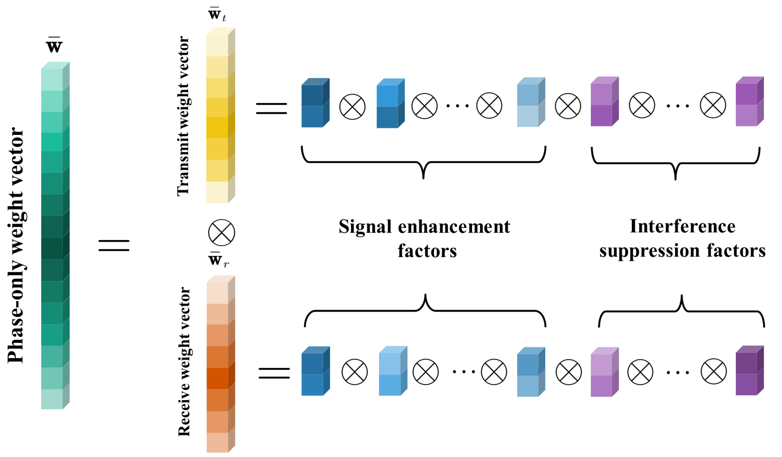
Now, we can design IS and SE factors separately to synthesize phase-only vector . For the convenience of understanding, we offer a relatively intuitive diagram Figure 2 where we can clearly see that the phase-only weight is decomposed into multiple Kronecker factors.
3.3.1. The Design of Interference Suppression Factors
As described in Problem (14), for any interference, the expected weight vector should satisfy Constraint (14c). Then, according to Equation (25), Constraint (14c) for jth interference steering vector is assumed to be
Using sets and , Equation (26) can be simply expressed as
where , .
One can observe from Equation (27) that for the jth interference, we only need to choose one of the Kronecker products, , such that the equation equals zero. Since is fixed, the selection process of Kronecker product is equivalent to selecting or from the set . The chosen is assigned to the corresponding Kronecker product factor in (27) for each jth interference equation, and is called the IS factor. We suppose the superscript of the chosen IS factor for the jth interference is ; based on Equation (27), the th Kronecker product factor should satisfy Equation (28).
where . We recall Equations (20) and (21); the specific form of can be defined as
For the jth equation, if , substituting (29) and (18) into (28), the unknown phase of the vector can be expressed as
If in the jth equation, substituting (29) and (19) into (28), the unknown phase of the vector can be expressed as
where and denote the transmit and receive spatial frequencies of the jth interference, respectively.
It is important to note that arbitrarily chosen satisfies Constraints (14d) or (14e), but not arbitrary can maximize the value of in (14b). Once the IS factors are determined, based on (25), can be written as
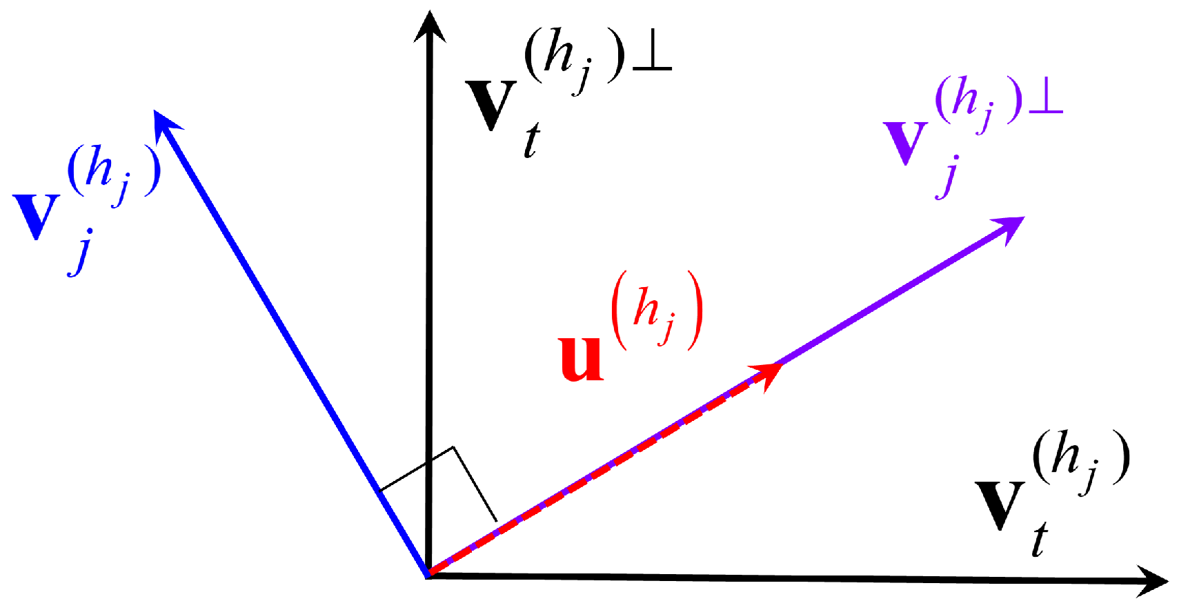
where . In order to design the weight vector and ensure maximizing in Constraint (14b), we expect (36) to be as large as possible. Thus, we calculate all the and choose with the largest modal value. The selected is able to obtain the maximum , that is, the target echo gain. For easy understanding of the relation between Kronecker factors and steering vector factors, the geometric perspective is shown in Figure 3. The calculated is actually in orthogonal space of , and the process of selecting is essentially to find orthogonal space with the smallest angle with .
In summary, the criterion for the determination of the IS factors effectively suppresses the interference signal while ensuring the maximization of the output SINR. The design procedure of IS factors is summarized in Algorithm 1 with specific steps elaborated.
| Algorithm 1 Design of IS factors. |
|
3.3.2. The Design of Signal Enhancement Factors
After obtaining the IS factors in , there are still SE factors to be designed. In other words, Kronecker product factors in need to be designed to maximize (enhanced signal power) and meet Constraints (14d) and (14e) (satisfy the phase-only constraint).
By pooling the designed IS factors corresponding to all J interferences, denoting the superscript of the SE factors as , Constraint (14b) can be expressed as
where and both belong to the set . Following Definitions (6) and (7) and Constraints (14d) and (14e), we can easily observe that the module of the th Kronecker product factor is not greater than 2. This implies that
Observing Equation (38), we know that obtains its maximum value only when and are conjugate with each other, i.e., . According to Definitions (18) and (19), we define to have the following form:
where or is chosen according to the value of ; and denote the transmit and receive spatial frequencies of the target, respectively.
Thus, when , the phase solutions to are
We note that arbitrarily satisfies Constraints (14d) or (14e). In summary, the SE factors can be determined, and steps are summarized in Algorithm 2.
| Algorithm 2 Design of SE factors |
|
With the two aforementioned algorithms, the SE and IS factors can be determined. The transmit and receive weight vectors can be calculated using the Kronecker product as specified in Equations (20) and (21), respectively. The final phase-only weight vector is calculated from Equation (13). Then, the design procedure of the phase-only weight vector is given in Algorithm 3.
| Algorithm 3 Design of Phase-Only Weight Vectors |
|
3.4. Discussion
In this subsection, we discuss the performance of the proposed phase-only beamforming algorithm, including the antenna number, IS factors selection, bistatic FDA-MIMO radar, and computation complexity.
3.4.1. Antenna Number
The weight vector is designed for the exceptional case when the number of transmitter and receiver and . In fact, for the general case of non-prime number, it can perform the Kronecker decomposition. After the Kronecker decomposition of and , they can be decomposed into Kronecker factors of the following form:
The transmit and receive weight vectors can be determined using the procedures described in the previous section.
According to reference [35], when the number of antennas is a prime number, one simple solution is to utilize antenna selection. This approach addresses the issue of the inability to decompose the steering vector into Kronecker products. For instance, in the case where there are 67 antennas, the optimal subset of 64 antennas can be chosen using a specific selection criterion. These selected 64 antennas can then be employed for phase-only beamforming using Kronecker decomposition. Additionally, it is mentioned in [35] that standards such as IEEE 802.11n and IEEE 802.11ac [36] often set the number of antennas to be a power of two. This aligns well with the proposed design, facilitating the application of the proposed approach.
3.4.2. Interference Suppression Factors Selection
In Algorithm 1, we consider the common case where each interference has different transmit and receive frequencies, that is, and . This means that the corresponding and for different interferences are not the same. Therefore, for the jth interference, the obtained can only be used to suppress the jth interference. If there are multiple interferences with a common transmit or receive frequency, it is possible to design an IS factor that can suppress both interferences simultaneously. This means that for different interferences, there is a shared component in (the transmit or receive Kronecker factors), and they have a common such that .
Moreover, it is important to note that the proposed algorithm exhibits a high demand for array DOFs due to the relationship between the number of IS and SE factors and the number of array elements. As the number of interferences increases, there is a degradation in beam performance for a given number of array elements. Furthermore, accurate a priori information is required by the proposed algorithm, indicating its limited robustness.
3.4.3. Bistatic FDA-MIMO Radar
In this subsection, we discuss the application of the proposed algorithm to a bistatic FDA-MIMO radar. According to the steps of the proposed algorithm, the calculation of the phase-only weight vector is related to the transmit and receive spatial frequencies of the interference and the target. For a bistatic FDA-MIMO radar, we let represent the direction of arrival and denote the direction of departure. The transmit and receive spatial frequencies of the bistatic FDA-MIMO radar are denoted as and , respectively. Therefore, when computing IS and SE factors in Algorithms 1 and 2, it is necessary to substitute the transmit and receive spatial frequencies with those of the bistatic FDA-MIMO radar.
3.4.4. Computation Complexity
It is worth highlighting that the proposed phase-only beamforming algorithm has low computational complexities. The computational cost of the algorithm primarily arises from the calculation of the phases of IS and the SE factors, including only the simple additions or multiplication operators. In the Algorithm 1 part, the computational complexity mainly arises from the calculation of phase solution and the calculation of . Since and with the dimension of , the computational complexity of is . The computational load of calculating the solution of in (33) or (35) is . So the computational complexity of Algorithm 1 is . In addition, the complexity of Algorithm 2 is . Based on the analyses above, the computational complexity of the proposed algorithm is , where . In contrast, the convex optimization method in [34] requires complex operations, and the SNBC method in [27] requires complex operations. Table 1 summarizes the computational complexity of these algorithms.
4. Simulation Results
In this section, we present numerical experiments to evaluate the effectiveness of the proposed method. Since the method in [34] cannot find an efficient solution in polynomial time when the number of antennas is large, we compare the performance of the proposed algorithm with that of the SNBC method [27] in this section. The main simulation parameters are provided in Table 2.
4.1. Beam Pattern for Different Interference Scenarios
In this subsection, we assess the effectiveness of the proposed algorithm in forming deep nulls at the desired locations.
4.1.1. One Suppression Point
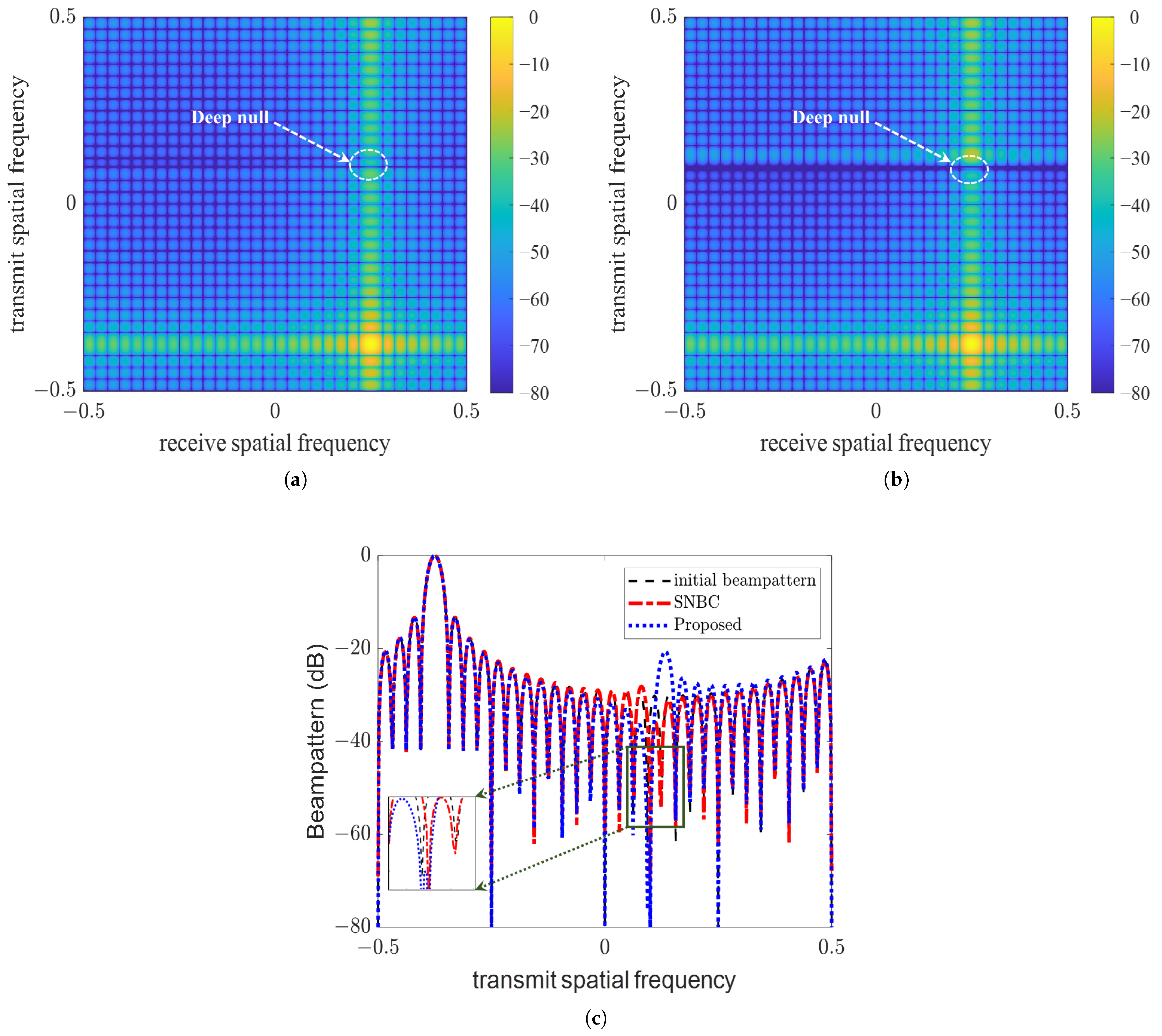
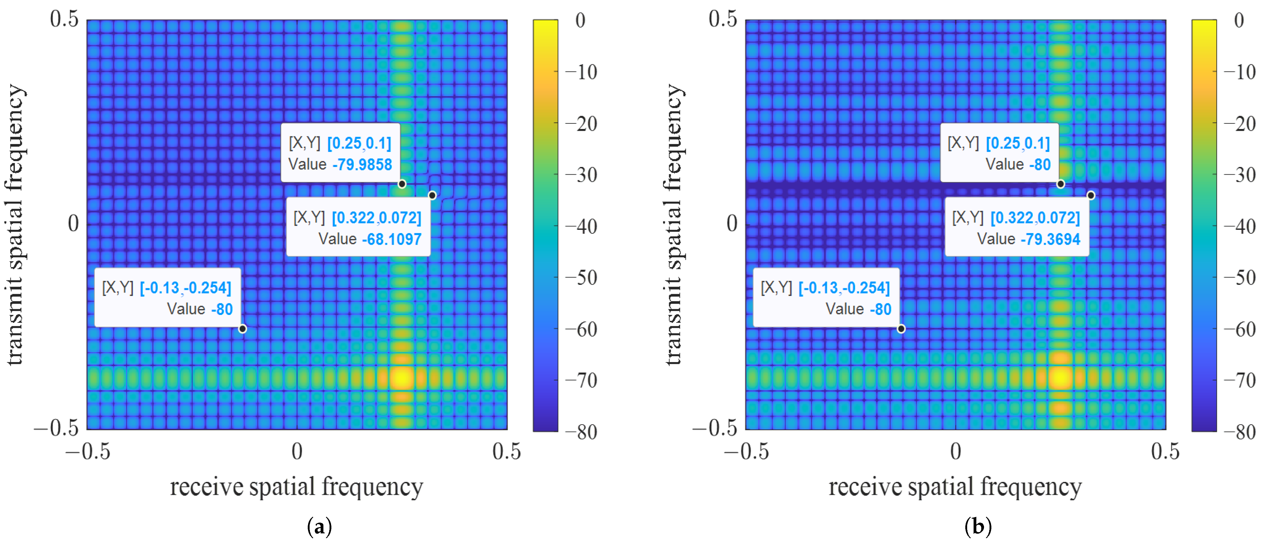
In the first example, we consider forming a deep null at one desired point . That is, the transmit frequency is 0.1, different from the target, and the receive frequency is 0.25, same as the target. Utilizing the proposed algorithmic procedure, we obtain the phase-only weight vectors. Table 3 offers transmit weight vector and receive weight vector , and the Kronecker product of the transmit and receive weight vectors is the final phase-only weight vector. By observing it, we can find that the obtained weight vector is phase only. Figure 4a,b plot the 2D beampattern synthesis result for different methods. Figure 4c produces the equivalent transmit beam pattern of a 2D beam pattern at the receive spatial frequency . One can observe that the two methods can effectively form a deep null in the desired position. Furthermore, it can be observed that our proposed method yields a higher sidelobe level compared to the SNBC method. This is determined by the performance of the proposed algorithm. However, it should be emphasized that the advantage of our algorithm is that the deep null beam pattern can be achieved solely by adjusting the phase of weight, a characteristic not possessed by the SNBC method.
4.1.2. Multiple Suppression Points
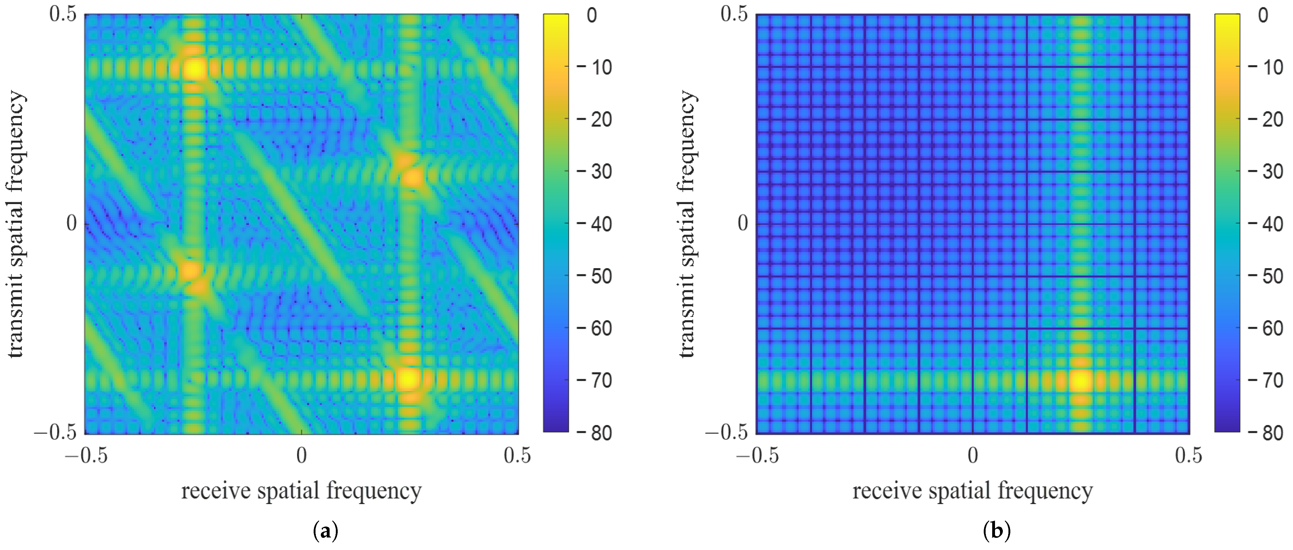
In the second example, a simulation experiment is designed to verify that the proposed algorithm can effectively form multiple deep nulls even in multiple desired positions. We consider three desired points with angle and range of ; and , respectively. The transmit and receive frequencies are , and , respectively. Figure 5 plots the 2D beampattern synthesis result by using phase-only weight. One can see that the proposed algorithm can effectively form three deep nulls in the corresponding interference positions. However, the SNBC method does not guarantee the formation of a deep zero at all points.
4.2. Beam Pattern on the Different Quantization Bits
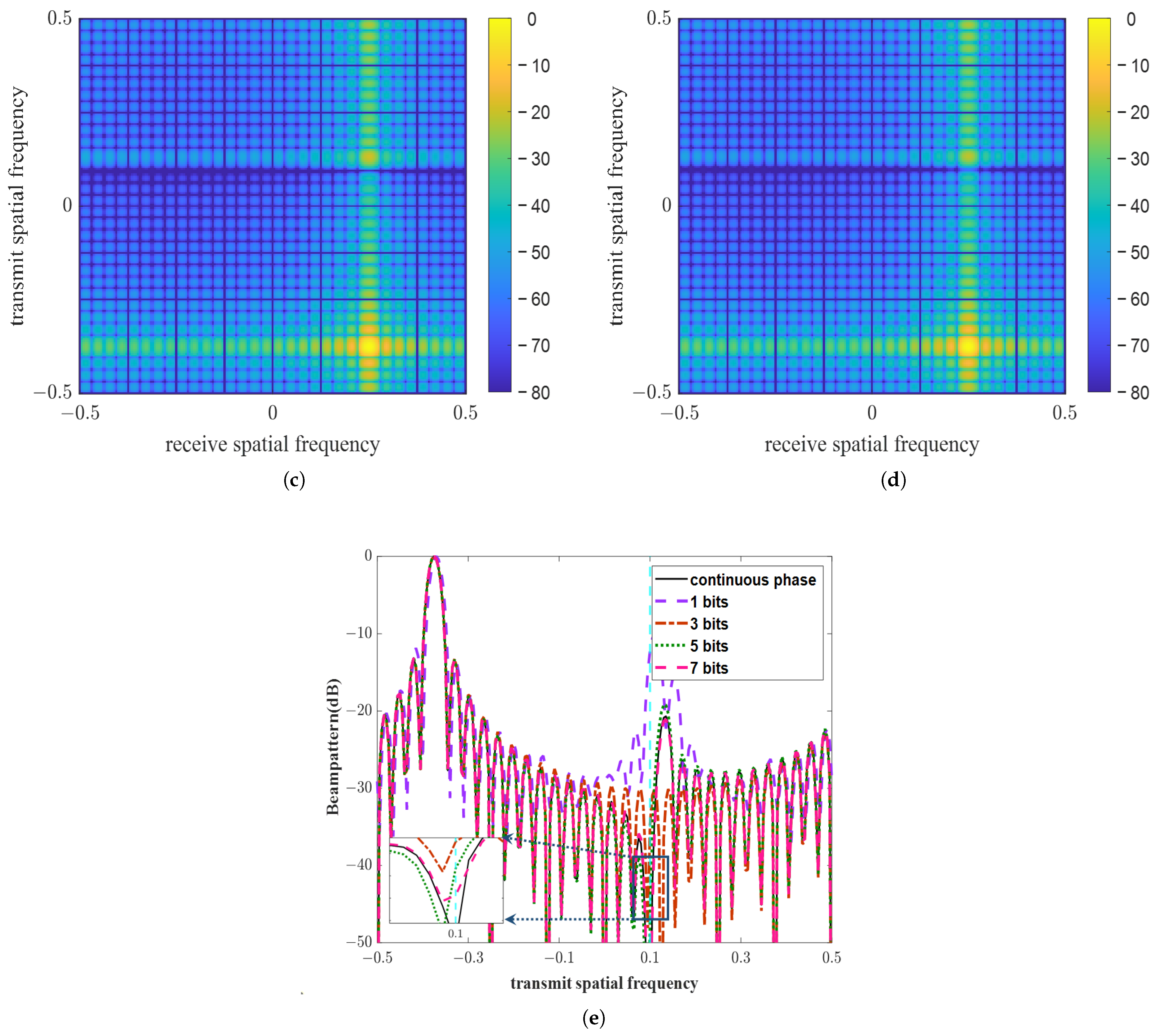
In practical applications, due to hardware limitations, phase shifters cannot generate a continuous phase; it is necessary to quantize the phase of the phase shifter. To show the performance of the beam pattern synthesized by our proposed algorithm on different quantization bits, the beampattern performances of the phase-only weight vector are compared in this subsection. Considering one suppression point, Figure 6 presents the beam pattern of the proposed algorithm when the receiver has different quantization bits, correspondingly. By observing the beam pattern, it can be observed that the quantized beam pattern exhibits considerable deviation from the original beam pattern when the receiver has different quantization bits. Especially when the quantization bit is one, the change in the beam pattern is more obvious. As the number of quantization bits increases, the quantized beam pattern gradually approaches the original beam pattern. For instance, when the quantization bit is seven, Figure 6d displays that the beampattern performance is roughly the same as the original beam pattern.
4.3. Output SINR on the Different Quantization Bits
In order to verify the output SINR performance of the proposed algorithm, we offer the output SINR at different signal to noise ratio (SNR) values and the number of snapshots. Furthermore, we present the output SINR on different quantization bits to show the performance of the proposed phase-only method when the phase shifters have different quantization bits. According to the constraints in (14), the output SINR is defined as
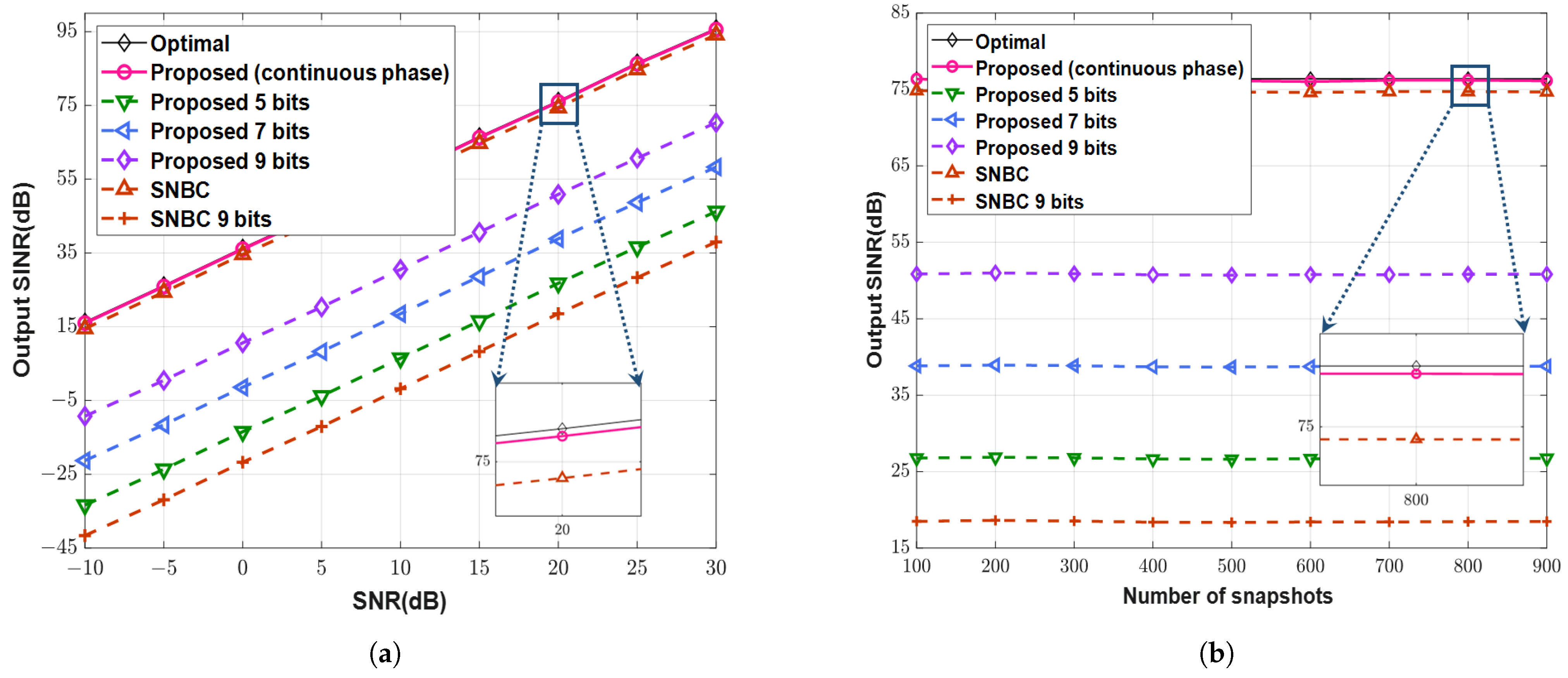
Considering one interference point with = 30 dB, Figure 7 provides the original output SINR of the proposed algorithm and the SNBC method [27]. Moreover, the output SINR values of the two algorithms are given in Figure 7 for different quantization bits. Since the SNBC algorithm is not phase only, here, we only show the quantized performance of the SNBC algorithm at nine bits. Specifically, Figure 7a displays the output SINR of the proposed method in the SNR from −10 dB to 30 dB with 800 snapshots; Figure 7b plots the output SINR in the number of snapshots from 200 to 900 under the SNR is 20dB.
One can see that the proposed algorithm has good performance. Compared to the optimal output SINR, the proposed method has only a little loss. The main reason is that we form a deep null at the interference position, which can effectively suppress the interference signal. Moreover, as the number of snapshots gradually increases, the output SINR of the proposed method does not change. This phenomenon occurs due to the fact that the proposed method is data independent. As shown in Figure 7, the output SINR of the proposed algorithm with different quantization bits is significantly different from the original output SINR. However, increasing the number of quantization bits brings the quantized SINR closer to the original performance. Moreover, since the SNBC method is not phase only, it can be seen that the quantized performance of the algorithm is poor at nine bits, but our proposed algorithm has better performance.
5. Conclusions
This paper proposed a fast phase-only beamforming algorithm based on Kronecker decomposition for the FDA-MIMO radar. We decomposed the phase-only weight vectors into transmit and receive weight vectors with Vandermonde structures. On this basis, the transmit and receive weight vectors were decomposed into Kronecker factors with uni-modulus vectors, which were further divided into IS and SE factors. We derived analytical solutions for both IS and the SE factors. The proposed algorithm is capable of obtaining a phase-only weight vector with low complexity. And the obtained phase-only weight vector can effectively form deep nulls at specific locations solely by adjusting the phase of receiver, thereby reducing the hardware costs of radar systems. As a future work, we will extend the proposed phase-only beamforming approach to the scenario with localization errors.
Author Contributions
Conceptualization, J.G.; Methodology, G.C. and J.G.; Formal analysis, C.W.; Investigation, M.T.; Writing—review & editing, M.T. All authors have read and agreed to the published version of the manuscript.
Funding
This work is supported in part by the National Natural Science Foundation of China under Grant 62201580, in part by the Natural Science Foundation of Shaanxi Province under Grant 2021JM-222 and 2023-JC-YB-553, in part by the Program of The Youth Innovation Team of Shaanxi Universities.
Data Availability Statement
The data used to support the findings of this study are available from the corresponding author upon request.
Conflicts of Interest
The authors declare no conflicts of interest.
References
- Zheng, Z.; Yang, T.; Wang, W.Q.; So, H.C. Robust Adaptive Beamforming via Simplified Interference Power Estimation. IEEE Trans. Aerosp. Electron. Syst. 2019, 55, 3139–3152. [Google Scholar] [CrossRef]
- Zhang, X.; He, Z.; Liao, B.; Zhang, X.; Yang, Y. Pattern Synthesis via Oblique Projection-Based Multipoint Array Response Control. IEEE Trans. Antennas Propag. 2019, 67, 4602–4616. [Google Scholar] [CrossRef]
- Ge, Q.; Zhang, Y.; Wang, Y.; Zhang, D. Multi-Constraint Adaptive Beamforming in the Presence of the Desired Signal. IEEE Commun. Lett. 2020, 24, 2594–2598. [Google Scholar] [CrossRef]
- Liang, C.; Zhang, X. Phased-Array Transmission for Secure Multiuser mmWave Communication via Kronecker Decomposition. IEEE Trans. Wirel. Commun. 2022, 21, 5744–5754. [Google Scholar] [CrossRef]
- Shi, J.; Wen, F.; Liu, Y.; Liu, Z.; Hu, P. Enhanced and Generalized Coprime Array for Direction of Arrival Estimation. IEEE Trans. Aerosp. Electron. Syst. 2023, 59, 1327–1339. [Google Scholar] [CrossRef]
- Su, X.; Liu, Z.; Shi, J.; Hu, P.; Liu, T.; Li, X. Real-Valued Deep Unfolded Networks for Off-Grid DOA Estimation via Nested Array. IEEE Trans. Aerosp. Electron. Syst. 2023, 59, 4049–4062. [Google Scholar] [CrossRef]
- Liu, J.; Liu, W.; Liu, H.; Chen, B.; Xia, X.G.; Dai, F. Average SINR Calculation of a Persymmetric Sample Matrix Inversion Beamformer. IEEE Trans. Signal Process. 2016, 64, 2135–2145. [Google Scholar] [CrossRef]
- Zhang, X.; He, Z.; Liao, B.; Zhang, X.; Peng, W. Pattern Synthesis with Multipoint Accurate Array Response Control. IEEE Trans. Antennas Propag. 2017, 65, 4075–4088. [Google Scholar] [CrossRef]
- Yujie, G.; Nathan, A.; Goodman, N.A.; Shaohua, H.; Li, Y. Robust adaptive beamforming based on interference covariance matrix sparse reconstruction. Signal Process. 2014, 96, 375–381. [Google Scholar]
- Ghayoula, R.; Fadlallah, N.; Gharsallah, A.; Rammal, M. Phase-only adaptive nulling with neural networks for antenna array synthesis. IET Microwaves Antennas Propag. 2009, 3, 154–163. [Google Scholar] [CrossRef]
- Van Luyen, T.; Vu Bang Giang, T. Interference Suppression of ULA Antennas by Phase-Only Control Using Bat Algorithm. IEEE Antennas Wirel. Propag. Lett. 2017, 16, 3038–3042. [Google Scholar] [CrossRef]
- Zhong, K.; Hu, J.; Cong, Y.; Cui, G.; Hu, H. RMOCG: A Riemannian Manifold Optimization-Based Conjugate Gradient Method for Phase-Only Beamforming Synthesis. IEEE Antennas Wirel. Propag. Lett. 2022, 21, 1625–1629. [Google Scholar] [CrossRef]
- Zhang, M.; Li, J.; Zhu, S.; Chen, X. Fast and Simple Gradient Projection Algorithms for Phase-Only Beamforming. IEEE Trans. Veh. Technol. 2021, 70, 10620–10632. [Google Scholar] [CrossRef]
- Zhang, X.; He, Z.; Liao, B.; Zhang, X. Fast Array Response Adjustment With Phase-Only Constraint: A Geometric Approach. IEEE Trans. Antennas Propag. 2019, 67, 6439–6451. [Google Scholar] [CrossRef]
- Chen, X.; Shu, T.; Yu, K.B.; He, J.; Yu, W. Joint Adaptive Beamforming Techniques for Distributed Array Radars in Multiple Mainlobe and Sidelobe Jammings. IEEE Antennas Wirel. Propag. Lett. 2020, 19, 248–252. [Google Scholar] [CrossRef]
- Cheng, Y.; Zhu, D.; Jin, G.; Zhang, J.; Niu, S.; Wang, Y. A Novel Intrapulse Repeater Mainlobe-Jamming Suppression Method with MIMO-SAR. IEEE Geosci. Remote Sens. Lett. 2022, 19, 4507805. [Google Scholar] [CrossRef]
- Bang, H.; Wang, W.Q.; Zhang, S.; Liao, Y. FDA-Based Space–Time–Frequency Deceptive Jamming Against SAR Imaging. IEEE Trans. Aerosp. Electron. Syst. 2022, 58, 2127–2140. [Google Scholar] [CrossRef]
- Wen, C.; Huang, Y.; Peng, J.; Wu, J.; Zheng, G.; Zhang, Y. Slow-Time FDA-MIMO Technique with Application to STAP Radar. IEEE Trans. Aerosp. Electron. Syst. 2022, 58, 74–95. [Google Scholar] [CrossRef]
- Tan, M.; Wang, C.; Li, Z. Correction Analysis of Frequency Diverse Array Radar about Time. IEEE Trans. Antennas Propag. 2021, 69, 834–847. [Google Scholar] [CrossRef]
- Wang, W.Q. Overview of frequency diverse array in radar and navigation applications. IET Radar Sonar Navig. 2016, 10, 1001–1012. [Google Scholar] [CrossRef]
- Lan, L.; Marino, A.; Aubry, A.; De Maio, A.; Liao, G.; Xu, J.; Zhang, Y. GLRT-Based Adaptive Target Detection in FDA-MIMO Radar. IEEE Trans. Aerosp. Electron. Syst. 2021, 57, 597–613. [Google Scholar] [CrossRef]
- Tan, M.; Gong, J.; Wang, C. Range Dimensional Monopulse Approach with FDA-MIMO Radar for Mainlobe Deceptive Jamming Suppression. IEEE Antennas Wirel. Propag. Lett. 2023, 1–5. [Google Scholar] [CrossRef]
- Xu, J.; Kang, J.; Liao, G.; So, H.C. Mainlobe Deceptive Jammer Suppression with FDA-MIMO Radar. In Proceedings of the 2018 IEEE 10th Sensor Array and Multichannel Signal Processing Workshop (SAM), Sheffield, UK, 8–11 July 2018; pp. 504–508. [Google Scholar] [CrossRef]
- Cheng, J.; Wang, W.Q.; Zhang, S. Joint MIMO and Frequency Diverse Array for Suppressing Mainlobe Interferences. In Proceedings of the 2020 International Symposium on Antennas and Propagation (ISAP), Osaka, Japan, 25–28 January 2021; pp. 171–172. [Google Scholar] [CrossRef]
- Xu, J.; Liao, G.; Zhu, S.; So, H.C. Deceptive jamming suppression with frequency diverse MIMO radar. Signal Process. 2015, 113, 9–17. [Google Scholar] [CrossRef]
- Lan, L.; Liao, G.; Jingwei, X.U.; Zhu, S.; Zhang, Y. Range-angle-dependent beamforming for FDA-MIMO radar using oblique projection. Sci. China Inf. Sci. 2022, 65, 152305. [Google Scholar] [CrossRef]
- Lan, L.; Liao, G.; Xu, J.; Zhang, Y.; Liao, B. Transceive Beamforming with Accurate Nulling in FDA-MIMO Radar for Imaging. IEEE Trans. Geosci. Remote. Sens. 2020, 58, 4145–4159. [Google Scholar] [CrossRef]
- Basit, A.; Wang, W.Q.; Wali, S.; Nusenu, S.Y. Transmit beamspace design for FDA–MIMO radar with alternating direction method of multipliers. Signal Process. 2021, 180, 107832. [Google Scholar] [CrossRef]
- Ding, Z.; Xie, J. Joint Transmit and Receive Beamforming for Cognitive FDA-MIMO Radar with Moving Target. IEEE Sens. J. 2021, 21, 20878–20885. [Google Scholar] [CrossRef]
- Gong, P.; Zhang, Z.; Wu, Y.; Wang, W.Q. Joint Design of Transmit Waveform and Receive Beamforming for LPI FDA-MIMO Radar. IEEE Signal Process. Lett. 2022, 29, 1938–1942. [Google Scholar] [CrossRef]
- Gao, K.; Shao, H.; Chen, H.; Cai, J.; Wang, W.Q. Impact of frequency increment errors on frequency diverse array MIMO in adaptive beamforming and target localization. Digit. Signal Process. 2015, 44, 58–67. [Google Scholar] [CrossRef]
- Zhou, C.; Wang, C.; Gong, J.; Bao, L.; Chen, G.; Liu, M. FDA-MIMO Radar Robust Beamforming Based on Matrix Weighting Method. IEEE Access 2022, 10, 58913–58920. [Google Scholar] [CrossRef]
- Lan, L.; Xu, J.; Liao, G.; Zhang, Y.; Fioranelli, F.; So, H.C. Suppression of Mainbeam Deceptive Jammer with FDA-MIMO Radar. IEEE Trans. Veh. Technol. 2020, 69, 11584–11598. [Google Scholar] [CrossRef]
- Chen, G.; Wang, C.; Gong, J.; Tan, M.; Liu, Y. Data-Independent Phase-Only Beamforming of FDA-MIMO Radar for Swarm Interference Suppression. Remote Sens. 2023, 15, 1159. [Google Scholar] [CrossRef]
- Zhu, G.; Huang, K.; Lau, V.K.N.; Xia, B.; Li, X.; Zhang, S. Hybrid Beamforming via the Kronecker Decomposition for the Millimeter-Wave Massive MIMO Systems. IEEE J. Sel. Areas Commun. 2017, 35, 2097–2114. [Google Scholar] [CrossRef]
- IEEE Std 802.11; IEEE Standard for Information technology—Telecommunications and Information Exchange between SystemsLocal and Metropolitan Area Networks—Specific requirements–Part 11: Wireless LAN Medium Access Control (MAC) and Physical Layer (PHY) Specifications–Amendment 4: Enhancements for Very High Throughput for Operation in Bands below 6 GHz. IEEE: Piscataway, NJ, USA, 2013; pp. 1–425. [CrossRef]
Figure 1.
The monostatic FDA-MIMO array structure.

Figure 2.
An abbreviated illustration of the design of the phase-only vector.

Figure 3.
Illustration of the Kronecker factors.

Figure 4.
The beam pattern for different methods. (a) SNBC [27]. (b) Proposed method. (c) The beam pattern at receive spatial frequency .
Figure 4.
The beam pattern for different methods. (a) SNBC [27]. (b) Proposed method. (c) The beam pattern at receive spatial frequency .

Figure 5.
The 2D beam pattern for different methods. (a) SNBC [27]. (b) Proposed method.
Figure 5.
The 2D beam pattern for different methods. (a) SNBC [27]. (b) Proposed method.

Figure 6.
The beam pattern on different quantization bits. (a) 1 bit, (b) 3 bits, (c) 5 bits, (d) 7 bits. (e) The beam pattern at receive spatial frequency .
Figure 6.
The beam pattern on different quantization bits. (a) 1 bit, (b) 3 bits, (c) 5 bits, (d) 7 bits. (e) The beam pattern at receive spatial frequency .


Figure 7.
The output SINR on different quantization bits. (a) The output SINR versus SNR. (b) The output SINR versus the number of snapshots.
Figure 7.
The output SINR on different quantization bits. (a) The output SINR versus SNR. (b) The output SINR versus the number of snapshots.


Table 1.
Comparison of Computational Complexity.
| Method | Computational Complexity |
|---|---|
| Convex optimization [34] | |
| SNBC [27] | |
| Proposed method |
Table 2.
Simulation parameters.
| Parameters | Symbols | Value |
|---|---|---|
| Transmit elements | N | 32 |
| Receive elements | M | 32 |
| Reference carrier frequency | 16 GHz | |
| Wavelength | 0.0187 m | |
| Frequency offset | 3750 Hz | |
| Main beam angle | ||
| Main beam range | 25 km | |
| Main beam transmit frequency | −0.375 | |
| Main beam receive frequency | 0.25 |
Table 3.
Phase-Only weight vector for one interference.
| 1 | 17 | ||||
| 2 | 18 | ||||
| 3 | 19 | ||||
| 4 | 20 | ||||
| 5 | 21 | ||||
| 6 | 22 | ||||
| 7 | 23 | ||||
| 8 | 24 | ||||
| 9 | 25 | ||||
| 10 | 26 | ||||
| 11 | 27 | ||||
| 12 | 28 | ||||
| 13 | 29 | ||||
| 14 | 30 | ||||
| 15 | 31 | ||||
| 16 | 32 |
Disclaimer/Publisher’s Note: The statements, opinions and data contained in all publications are solely those of the individual author(s) and contributor(s) and not of MDPI and/or the editor(s). MDPI and/or the editor(s) disclaim responsibility for any injury to people or property resulting from any ideas, methods, instructions or products referred to in the content. |
© 2024 by the authors. Licensee MDPI, Basel, Switzerland. This article is an open access article distributed under the terms and conditions of the Creative Commons Attribution (CC BY) license (https://creativecommons.org/licenses/by/4.0/).
Share and Cite
MDPI and ACS Style
Chen , G.; Wang , C.; Gong , J.; Tan , M. A Fast Phase-Only Beamforming Algorithm for FDA-MIMO Radar via Kronecker Decomposition. Electronics 2024, 13, 337. https://doi.org/10.3390/electronics13020337
AMA Style
Chen G, Wang C, Gong J, Tan M. A Fast Phase-Only Beamforming Algorithm for FDA-MIMO Radar via Kronecker Decomposition. Electronics. 2024; 13(2):337. https://doi.org/10.3390/electronics13020337
Chicago/Turabian StyleChen , Geng, Chunyang Wang , Jian Gong , and Ming Tan . 2024. "A Fast Phase-Only Beamforming Algorithm for FDA-MIMO Radar via Kronecker Decomposition" Electronics 13, no. 2: 337. https://doi.org/10.3390/electronics13020337
Note that from the first issue of 2016, this journal uses article numbers instead of page numbers. See further details here.