Penetration State Identification of Aluminum Alloy Cold Metal Transfer Based on Arc Sound Signals Using Multi-Spectrogram Fusion Inception Convolutional Neural Network

Abstract

The CMT welding process has been widely used for aluminum alloy welding. The weld’s penetration state is essential for evaluating the welding quality. Arc sound signals contain a wealth of information related to the penetration state of the weld. This paper studies the correlation between the frequency domain features of arc sound signals and the weld penetration state, as well as the correlation between Mel spectrograms, Gammatone spectrograms and Bark spectrograms and the weld penetration state. Arc sound features fused with multilingual spectrograms are constructed as inputs to a custom Inception CNN model that is optimized based on GoogleNet for CMT weld penetration state recognition. The experimental results show that the accuracy of the method proposed in this paper for identifying the fusion state of CMT welds in aluminum alloy plates is 97.7%, which is higher than the identification accuracy of a single spectrogram as the input. The recognition accuracy of the customized Inception CNN is improved by 0.93% over the recognition accuracy of GoogleNet. The customized Inception CNN also has high recognition results compared to AlexNet and ResNet.

1. Introduction

Cold Metal Transfer (CMT) is a modified Melt Inert-Gas/Metal Argon Gas (MIG/MAG) welding short-circuit transition welding process [1]. The waveforms of the voltage and current during welding are controlled by a digital control system. During short-circuiting, the current and current drop to zero, the heat input is reduced, and the transition of the molten drop is accomplished by the mechanical movement of the wire retraction. Compared with the traditional welding process, the CMT welding process is characterized by an accurate energy input control, a stable arc length, no spatter, etc. It is widely used for thin plate welding, dissimilar metal welding, Wire Arc Additive Manufacturing (WAAM) and so on [2,3,4,5]. In the CMT automated welding process, the real-time detection of the quality of the weld seam is the key to improving productivity and controlling product quality.

The penetration state of the weld is an important indicator for evaluating the quality of the weld. Arc welding is a complex physical and chemical process. The weld molten pool, arc voltage and current, as well as the arc sound and arc light produced by the weld, contain a great deal of relevant information on the different states of penetration, such as non-penetration, full penetration, excessive penetration and burned through. In automated welding processes, researchers use various sensor technologies to capture the arc sound signals [6,7,8,9], electrical signals [10,11] and molten pool images [12,13] for weld defect identification. The molten pool image visually reflects the quality of the weld seam, but aluminum alloys have high reflectivity, making the molten pool image difficult to acquire and process, and the camera is large in size, so the use of the scene receives certain limitations. Among various sensing technologies, sound sensors are small in size and applicable to more scenarios, and arc sound signals can easily collect and contain abundant information related to the weld quality. Therefore, studying the relationship between the arc sound signal and weld quality has been gradually emphasized by scholars; the relationship between gas tungsten arc welding (GTAW), arc sound signal and weld penetration state has been studied, and some results have been achieved [14,15,16]. However, due to the complexity of the CMT welding process, there have been fewer studies on the relationship between the CMT welding arc’s sound signal and the weld’s quality [17,18], especially in the field of aluminum alloys.

In the research on welding defect recognition based on arc sound, the Short-Time Fourier Transform (STFT) and Mel-Frequency Cepstral Coefficients (MFCCs) methods are commonly used to extract the features of arc sound signals and combine them with deep learning models such as Convolutional Neural Networks (CNNs) or Long Short-Term Memory (STML) networks for welding defect recognition [15,16,17,18]. Different sound feature extraction methods also have large effects on the recognition results of the model. The Mel filter bank, Gammatone filter bank and Bark filter bank are commonly used to extract the time–frequency domain features of speech signals [19,20,21]. The Mel filter bank is also used to extract the time–frequency domain features of welding arc sound signals [17]. However, the use of the Gammatone filter bank and Bark filter bank for arc sound time–frequency feature extraction is rarely reported. CNN’s GoogleNet is commonly used for image classification [22,23], but few reports have been made on the classification of sound signals, especially the classification of arc sound signals.

In this study, the spectrograms of arc sound signals were extracted using the Mel filter bank, Gammatone filter bank and bark filter bank. The three extracted spectrograms were fused, and then the fused spectrograms were input into the optimized lightweight GoogleNet for CMT aluminum alloy butt weld penetration state recognition. The remainder of the paper is organized as follows: Section 2 describes the methods for the spectrogram extraction and fusion of arc sound signals and the customized Inception CNN model [22]. Section 3 describes the design of the welding experiments and the acquisition process of the welding arc sound signals, as well as the construction of the dataset and the training and testing process of the network model. In Section 4, the effects of different datasets on the classification results are discussed and analyzed, and the proposed method is compared with other classification methods. Finally, Section 5 summarizes the main conclusions.

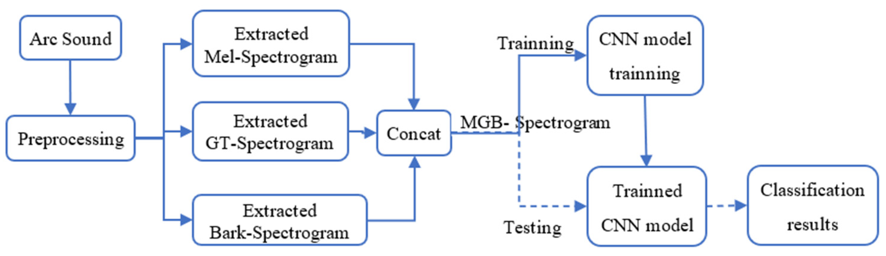
2. The Proposed Method

In order to obtain more features of the arc acoustic signal, the method proposed in this paper is shown in Figure 1. Firstly, the Mel spectrogram (Mel–Spectrogram), Gammatone spectrogram (GT–Spectrogram) and Bark spectrogram (Bark–Spectrogram) of the preprocessed arc sound signals are extracted separately, and the extracted spectrograms are concatenated to generate fused spectrograms (MGB–Spectrogram). Then, the MGB–Spectrogram is input into the customized Inception CNN model for training. Finally, the MGB–Spectrogram used for testing is input into the trained model to obtain the classification results.

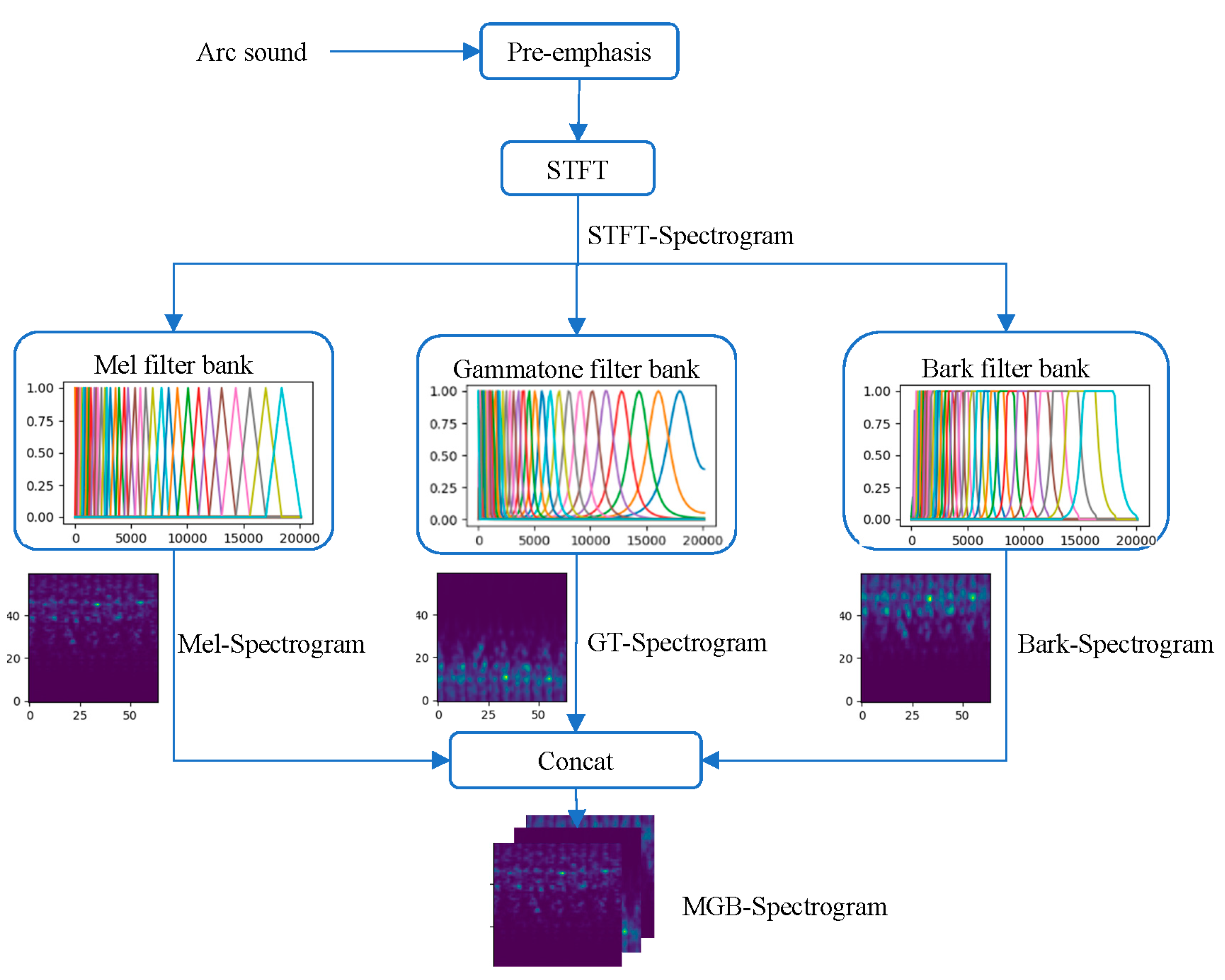
2.1. Arc Sound Feature Extraction

Feature extraction is a critical step in classification and recognition using deep learning algorithms. The Mel filter bank, Gammatone filter bank and Bark filter bank are used to extract the spectrograms of sound signals in speech recognition and classification studies based on sound signals [24,25,26,27]. In order to extract richer features, a method for extracting fusion spectrograms is proposed, as shown in Figure 2.

• Pre-emphasis

The arc sound signal is pre-emphasized to enhance the high-frequency component of the signal. The pre-emphasis formula is shown in Equation (1):

$$x^{\prime }\left(n\right)=x\left(n\right)+\alpha x(n-1)$$

(1)

where the coefficient α is in the set [0.9 to 1]. In this study, α takes the value of 0.97.

2.

Short-time Fourier Transform (STFT)

STFT is a joint time–frequency analysis method for time-varying unsteady signals [28], which can transform a 1D arc sound signal into a 2D spectrogram.

Firstly, the framing and windowing process is performed. The arc sound signal can be regarded as a steady process in a short time, so it is necessary to divide the signal into a number of frames of length N. Adjacent frames are partially overlapped to smooth the changes in the feature parameters of neighboring frames. In order to minimize spectral leakage, each frame needs to be operated using a window function. The formulas for framing and windowing the signal are given in Equation (2):

$$x_l\left(n\right)=x^{\prime }\left(n+lD\right)w\left(n\right) , 0\le n\le N-1$$

(2)

where $w\left(n\right)$ is the window function, $l$ is the index of the frame, $D$ is the distance between adjacent frames and N is the length of the window function, which is the frame length.

Secondly, the spectra of each frame are obtained by Discrete Fourier Transform (DFT), and these spectra are stitched together as column vectors along the horizontal direction to generate a two-dimensional spectrogram. The DFT formula is shown in Equation (3).

$$X_l\left(k\right)=\sum _{n=0}^{N-1}{x}_l\left(n\right)e^{-j\frac{2k\pi }{N}}, 0\le k\le N$$

(3)

where $l$ is the index of the frame, $k$ is the index of frequency and $X_l\left(k\right)$ is the spectra of the $l\mathrm{t}\mathrm{h}$ frame.

3.

Filtering and spectrogram fusion

The Mel filter bank is a triangular filter bank based on the Mel scale. This simulates the nonlinear perception of sound frequencies by the human ear [29]. The filters in the Mel filter bank become denser the closer they are to the lower frequencies, and these filters become sparser the closer they are to the higher frequencies. Thus, a nonlinear perception of frequency is achieved. The Gammatone filter bank simulates the response of the cochlea to a sound signal. The formula for the time–domain impulse response of the Gammatone filter is shown in Equation (4) [30].

$$g\left(t\right)=t^{p-1}{e}^{-\left[2\pi tb\right(f_c\left)\right]}\cos \left[2\pi f_c\right]; t\ge 0$$

(4)

where t denotes the time; $p$ is the order of the filter, which is set to 4 in this paper; $f_c$ is the center frequency of the filter and $b\left(f_c\right)$ is the bandwidth of the filter, centered at frequency $f_c$. The Bark filter bank simulates the psychological perception of sound loudness in humans [31].

The STFT spectrogram was processed using the Mel filter bank, Gammatone filter bank and Bark filter bank to obtain the Mel, Gammatone and Bark spectrograms, respectively. The formula used to process the STFT spectrum using a filter bank is shown in Equation (5):

$$S_l\left(i\right)=\sum _{k=0}^{N-1}{\left|X_l\left(k\right)\right|}^2{F}_i\left(k\right)$$

(5)

where $X_l\left(k\right)$ is the spectra of the $l\mathrm{t}\mathrm{h}$ frame, $F_i\left(k\right)$ is the $i\mathrm{t}\mathrm{h}$ filter of the Mel, Gammatone or Bark filter bank and $S_l\left(i\right)$ is the Mel spectrogram, Gammatone spectrogram or Bark spectrogram.

The widths of the Mel–Spectrogram, GT–Spectrogram and Bark–Spectrogram are equal to the amount of frames, and the heights are equal to the number of filters. Overlapping Mel–Spectrogram, GT–Spectrogram and Bark–Spectrogram of the same scale constitute a three-dimensional MGB–Spectrogram, which is used as an input for the customized model.

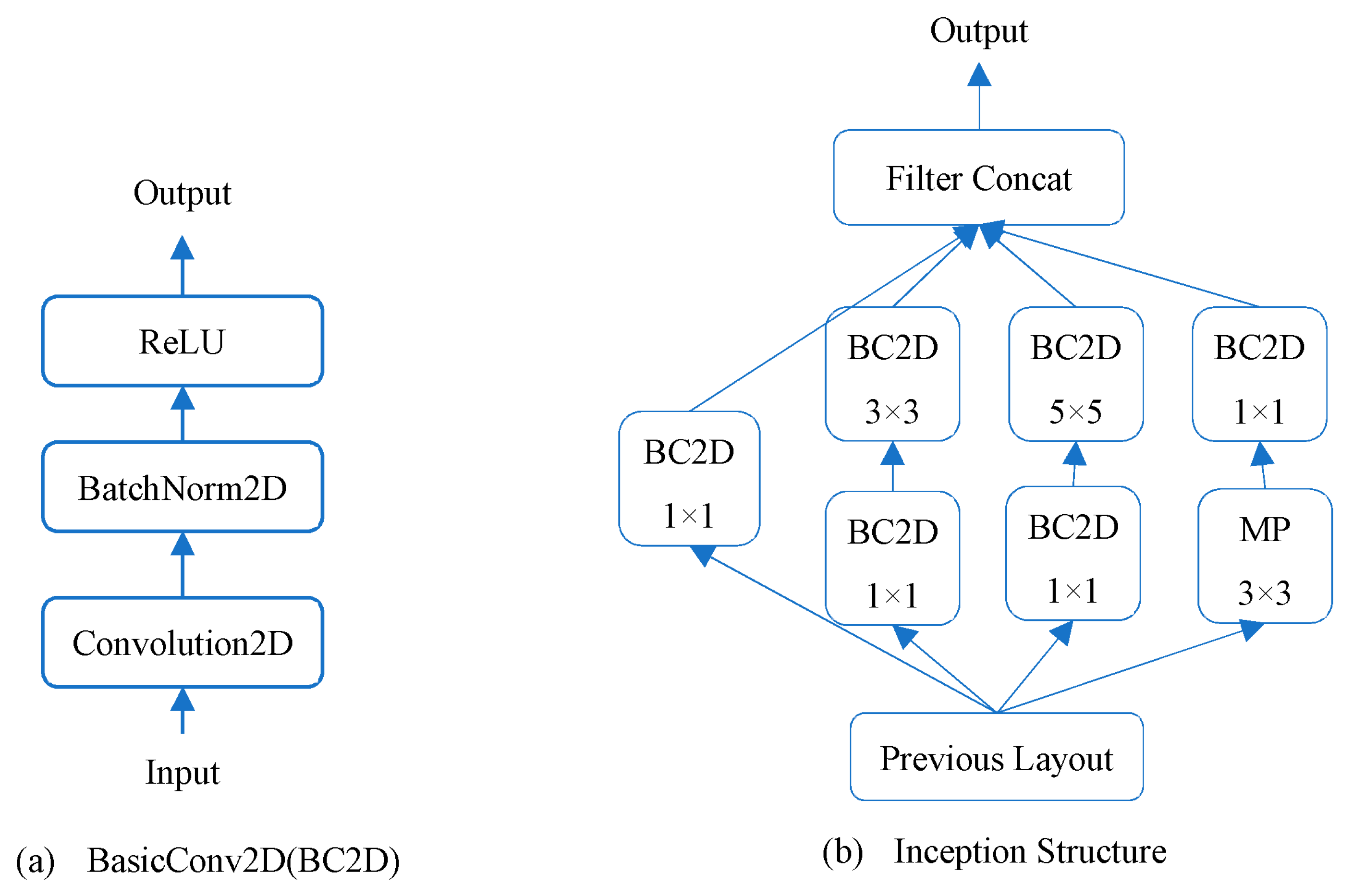
2.2. Inception CNN Classification Model

CNN is widely used as a deep learning model for welding defect recognition [32,33,34]. The structure of the CNN mainly consists of a convolutional layer, activation function, pooling layer and fully connected layer [35,36]. The convolutional layer extracts features from the local region of the input map using a certain size of a convolutional kernel, and these extracted local features constitute a feature map; this feature map will be used as an input for later layers. Different convolutional kernels can extract different feature maps. Multiple different features of the input map can be extracted by multiple convolutional kernels. The activation function increases the expressive and learning capabilities of the CNN through nonlinear operations. Typical activation functions are sigmoid, tanh and ReLU. The pooling layer improves the generalization of the CNN by down sampling, and the typical pooling operations are maximum pooling and average pooling.

The GoogleNet model is a deep CNN that introduces an Inception structure that is capable of fusing feature information at different scales, which has obtained good prediction results in the field of image recognition [22]. However, GoogleNet has a relatively large depth, and the parameters and operations of its model are quite large, requiring substantial computing resources. The custom Inception CNN model in this paper is a lightweight GoogleNet model that reduces the number of layers in the network, removes the auxiliary classifier structure, and adds a batch normalization [37] layer between each convolutional layer and the activation function to increase the stability and learning speed of the model.

The customized Inception CNN structure used in this paper is shown in

Table 1. Customized Inception CNN architecture.

No.	Component	Output Size
0	Input	C × H × W
1	BasicConv2D (C, 64, 7, 1, 3)	64 × H × W
2	MaxPool (64, 64, 3, 2, 1)	64 × ⎡H/2⎤ × ⎡W/2⎤
3	BasicConv2D (64, 64, 1, 1, 0)	64 × ⎡H/2⎤ × ⎡W/2⎤
4	BasicConv2D (64, 64, 3, 1, 1)	64 × ⎡H/2⎤ × ⎡W/2⎤
5	MaxPool (64, 192, 3, 2, 1)	192 × ⎡H/4⎤ × ⎡W/4⎤
6	InceptionModel (192, 64, (96, 128), (16, 32), 32)	256 × ⎡H/4⎤ × ⎡W/4⎤
7	InceptionModel (256, 128, (128, 192), (32, 128), 64)	512 × ⎡H/4⎤ × ⎡W/4⎤
8	MaxPool (512, 3, 2, 1)	512 × ⎡H/8⎤ × ⎡W/8⎤
9	InceptionModel (512, 256, (160, 320), (32, 128), 128)	832 × ⎡H/8⎤ × ⎡W/8⎤
10	InceptionModel (832, 256, (192, 512), (64, 128), 128)	1024 × ⎡H/8⎤ × ⎡W/8⎤
11	AdaptiveAvgPool2d (1024, (1, 1))	1024 × 1 × 1
13	FullConnection (1024, 3)	3
0	Input	C × H × W

. In Table 1, BasicConv2D denotes a convolutional module consisting of a convolutional layer, a batch normalization layer and the activation function ReLU, as shown in Figure 3a. The BasicConv2D module has five parameters: the first parameter represents the number of channels of the input feature map, the second parameter represents the number of channels of the output feature map, the third parameter represents the size of the convolution kernel, the fourth parameter represents the step size of the convolution kernel move and the last parameter represents the size of the padding around the feature map. MaxPool is maximum pooling, and its five parameters have the same meaning as the BasicConv2D module. The Inception Model in Table 1 represents an Inception structure, as shown in Figure 3b. In Figure 3b, the numbers in rounded rectangles indicate the size of the convolution kernel. In the Inception structure, branches with convolutional kernels of different sizes have different receptive fields and can extract richer features [22]. The InceptionModel has five parameters: the first parameter is the number of channels in the input feature map, and the next four parameters are the number of channels in the output feature map of each branch of the Inception structure.

3. Experiment

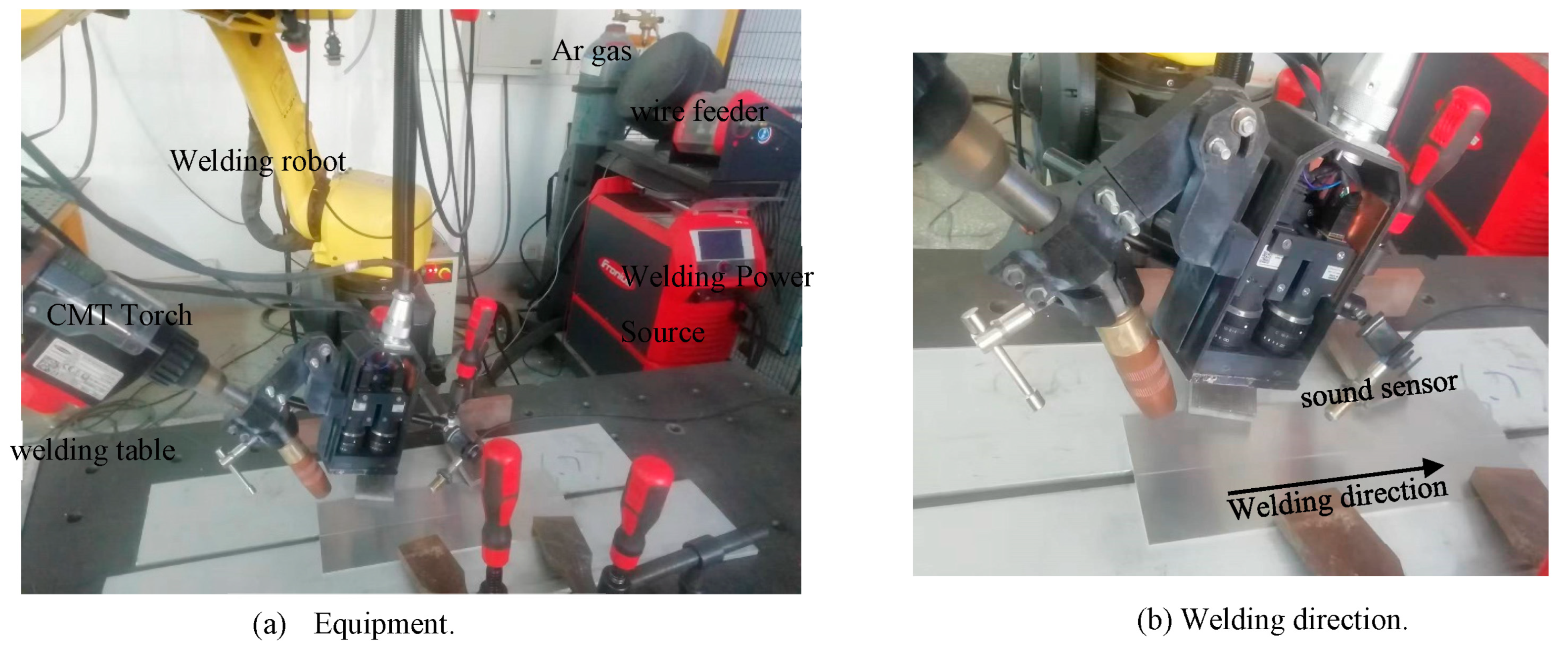
3.1. Welding Experiments

The welding experimental setup for welding arc sound signal acquisition is shown in Figure 4. The experimental setup consists of a welding system, a welding robot, a sensor system and a computer. The welding system includes a welding power source (Fronius TPS 600i, the equipment was manufactured by Fronius International GmbH in Austria and sourced from Fronius China Trading Co., Ltd. (Shanghai, China)), CMT torch, wire feeder, welding table and other accessories. The sensor system consists of an audio sensor and a signal acquisition card. The sound sensor is a Yawei Z1 noise sensor, and the data acquisition card is an Advantech USB4711 data acquisition card. During the welding process, the welding robot controls the welding path, and the sound sensor is located directly in front of the welding path in a synchronized motion with the welding torch, as shown in Figure 4b. The data acquisition card converts the arc sound signal and electrical signal captured by the sensor into a digital signal with a sampling frequency of 40 kHz.

Welding experiments were carried out using the DC CMT welding process for butt joint 6061 aluminum alloy plate. The size of the aluminum alloy plate is 300 mm × 50 mm × 2 mm. The shielding gas is high-purity argon (99.999%) with a flow rate of 15 mL/min. The diameter of the welding wire ER5356 is 1.2 mm.

Welding defects occur randomly during the welding process. In order to obtain arc sound signals for different penetration states, welding experiments were carried out according to the welding parameters shown in

Table 2. Welding experimental parameters and penetration states.

No.	Current (A)	Voltage (V)	Welding Speed (m/min)	Wire Feed Speed (m/min)	Gap (mm)	Penetration State
1	78	12.6	40	5.8	0	non-penetration, full penetration
2	78	12.6	40	5.8	1	non-penetration, full penetration
3	95	13.5	40	6.7	1	excessive penetration
4	98	13.7	35	6.9	1	excessive penetration
5	85	13	40	6.2	1	full penetration
6	85	13	40	6.2	0	full penetration
7	78	12.6	40	5.8	0	non-penetration, full penetration

. Three penetration states were obtained: non-penetration, full penetration and excessive penetration. Figure 5 shows the weld and its arc sound signals for different penetration states.

3.2. Building and Dividing the Dataset

The arc sound signals collected in Section 3.1 were segmented, with 3784 points per segment, to obtain 2277 arc sound segments, constituting the original dataset. This contains 768 non-penetration samples, 1509 full penetration samples and 936 excessive penetration samples. The Mel spectrogram dataset, GT spectrogram dataset, Bark spectrogram dataset and MGB spectrogram dataset were obtained by processing the arc sound segments in the original dataset according to the method in Section 2.1.

The STFT uses a Hanning window with a length of 256 to divide the arc sound segment into 64 frames, each containing 256 points, with 200 points overlapping in adjacent frames. The STFT spectrogram was filtered using the Mel filter bank, Gammatone filter bank and Bark filter bank containing 40, 50, 60, 70, 80, 90 or 100 filters, respectively, to obtain different results. The Mel–Spectrogram, GT–Spectrogram, Bark–Spectrogram and MGB–Spectrogram and the corresponding datasets are denoted as Mel-n, GT-n, Bark-n and MGB-n, respectively, with n denoting the number of filters.

Each constructed dataset was split into a training dataset (70%) and a testing dataset (30%). The proportion of samples with different fusion states in the training dataset set and testing dataset is the same as that in the original dataset.

3.3. Welding Defect Recognition

The network model customized in Section 2.2 was trained and tested using the training and testing datasets constructed in Section 3.2 as the input. In the model training process, the number of epochs was 100, the batch size was 64, the optimizer used Adam [38] and the learning rate formula was as shown in Equation (6):

$$lr={lr}_{init}\times {\gamma }^{\frac{epoch}{step}}$$

(6)

where $lr$ denotes the learning rate, ${lr}_{init}$ is the initial learning rate, γ denotes the decay coefficient of the learning rate and the range is [0, 1]; step denotes the step size of the learning rate decay. In this study, ${lr}_{init}$ is 0.001, γ is 0.9 and step is 10.

4. Results and Discussion

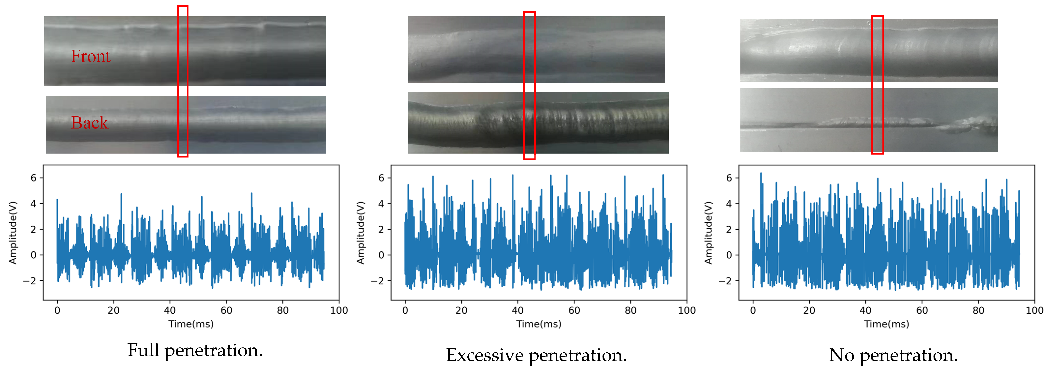
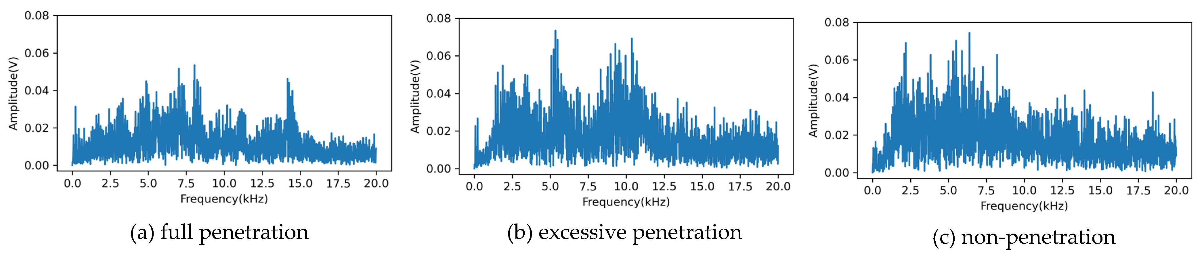
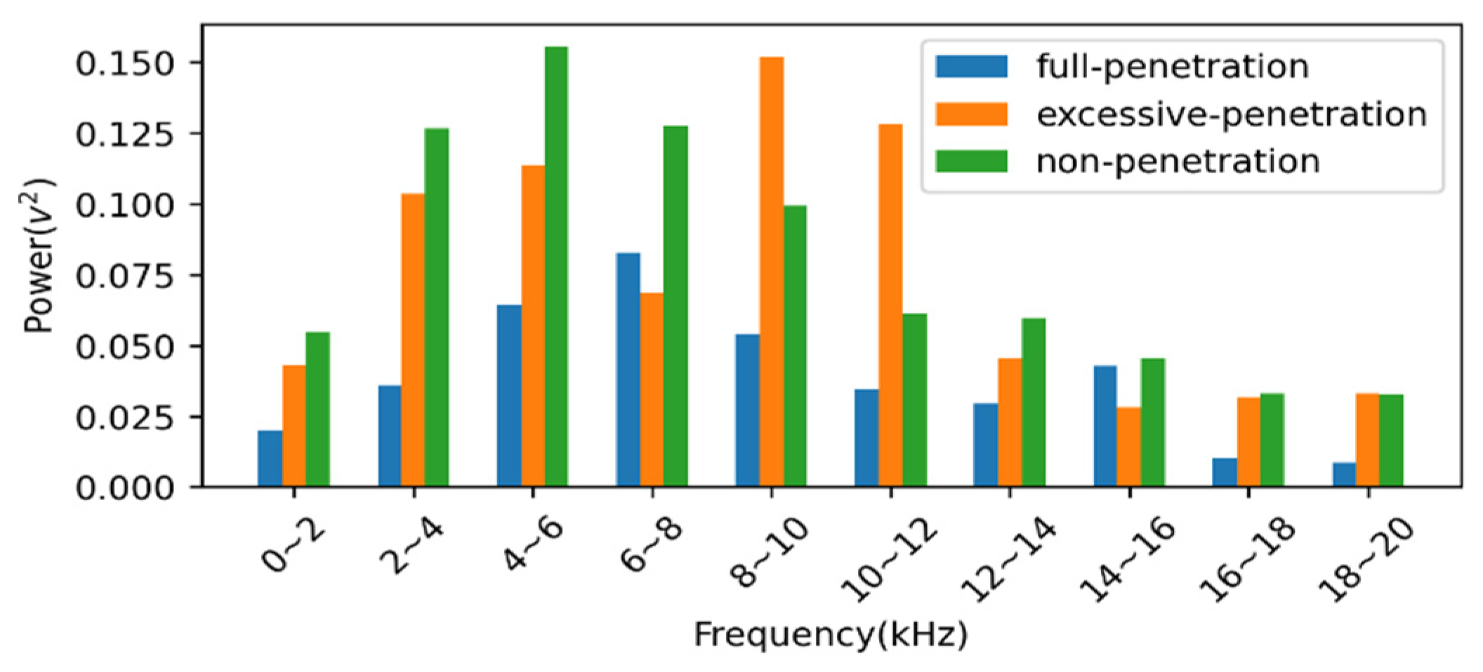
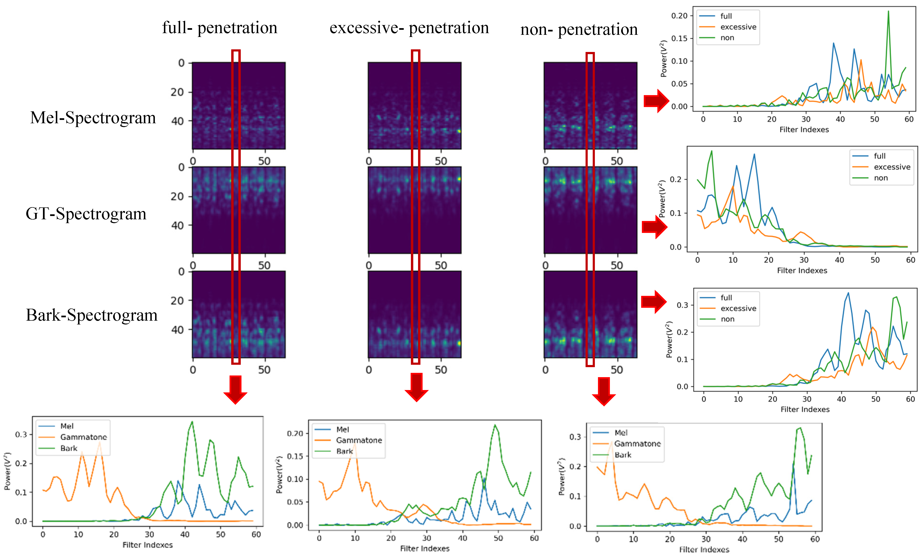
4.1. Arc Sound Frequency Analysis

Figure 5 shows the weld appearance and the corresponding arc sound time–domain signals for different penetration states. As can be seen in Figure 5, the time–domain signals of the arc sound in three different penetration states show periodic vibrations, but their amplitude strengths differ, with the excessive penetration and non-penetration arc sound signals vibrating strongly and having larger maximum amplitudes.

Figure 6 shows the frequency domain signal of the arc sound. Figure 6 shows that the main frequency components of the full penetration state are concentrated within 0 kHz~15 kHz, with multiple peaks in this range, the main frequency components of the excessive penetration state are concentrated within 1.5 kHz~12 kHz, with three peaks in this range, and the main frequency components of the non-penetration state are concentrated within 1.5 kHz~10 kHz. The frequency components of the three penetration states are more complex and do not show clear periodicity. The frequency overlap between three penetration states is large. There may be differences in amplitudes for different penetration states, with larger amplitudes for excessive penetration and non-penetration.

Figure 7 compares the frequency domain distribution of the arc sound energy for different penetration states. The energy of the arc sound for the three different penetration states in each frequency range in Figure 7 is also significantly different. In the band ranges of the previous seven, the three penetration states’ arc sound energies are obviously different, especially in the frequency ranges of 4 kHz~6 kHz and 8 kHz~10 kHz.

4.2. Effect of Number of Filters on Recognition Accuracy

In the arc sound signal feature extraction, filter banks containing different numbers of filters will generate spectrograms of different sizes, and the feature information contained in the spectrograms will be different. The MGB-40, MGB-50, MGB-60, MGB-70, MGB-80, MGB-90 and MGB-100 datasets are used as inputs for the customized Inception CNN model, respectively, and the model recognition accuracies are obtained for each dataset. Accuracy is a simple metric for evaluating the performance of the model, and its formula is shown in Equation (7):

$$Accuracy=\frac{cp}{sampl\_size}$$

(7)

where $cp$ denotes the number of correctly predicted samples in the test dataset, and $sampl\_size$ denotes the total number of samples in the test dataset.

Figure 8 compares the average test accuracy of recognition for seven datasets. Figure 8 shows that the average test accuracy of each dataset is greater than 97.00%. The MGB-60 dataset has the largest average test accuracy of 97.70%, and the MGB-80 dataset has the smallest average test accuracy of 97.01%. This shows that increasing the number of filters in the filter bank does not extract more features to improve the classification accuracy.

Table 3. Standard deviation of average test accuracy.

Dataset	MGB-40	MGB-50	MGB-60	MGB-70	MGB-80	MGB-90	MGB-100
Standard Deviation	0.23	0.29	0.12	0.10	0.36	0.30	0.30

shows the standard deviation of the average test accuracy for the different datasets. Table 3 shows that the standard deviation of MGB-60 is smaller, indicating that the features extracted by the filter bank with 60 filters are more stable.

4.3. Multilingual Spectrogram Fusion Analysis

Figure 9 compares the Mel–Spectrogram, GT–Spectrogram and Bark–Spectrogram of the arc sound for three different penetration states. Each filter bank that is used contains 60 filters. In Figure 9, the horizontal coordinate of each spectrogram is the frame index, and the vertical coordinate is the filter index. The line graph below compares the results of the 32nd frame of the different spectrograms for the same penetration state, and the line graph on the right compares the results of the 32nd frame of different penetration state spectrograms for the same filter bank. As can be seen in Figure 9, the Mel–Spectrogram, GT–Spectrogram and Bark–Spectrogram of the same penetration state are obviously different. The main features of the Mel–Spectrogram and Bark–Spectrogram are extracted by filters between the 30th and 60th, and the main features of the GT–Spectrogram are extracted by filters between the 1st and 30th. The spectrograms of the same filter bank for different penetration states are also obviously different. An obvious difference in the filtering results for different penetration states can also be seen in the line graph on the right side.

Figure 10 compares the average test accuracies for the Bark-60, GT-60, Mel-60 and MGB-60 datasets. The Gam-60 dataset has a higher average test accuracy than the Bark-60 and the Mel-60 datasets. This is because the Gammatone filter bank simulates the cochlear perception of sound and is robust to noise. Thus, the GT-60 dataset contains richer arc sound features. The MGB-60 dataset has the largest average test accuracy. This is because the Mel filter bank, Gammatone filter bank, and Bark filter bank extract different features from the arc sound, and the MGB-60 dataset fuses the features extracted by the three filter banks, and therefore has richer features.

Table 4. Standard deviation of dataset test accuracy.

Dataset	Bark-60	GT-60	Mel-60	MGB-60
Standard Deviation	0.005	0.002	0.004	0.001

shows the standard deviation of the recognition accuracies of the four datasets, with MGB-60 being the smallest.

4.4. Comparison with Other Classification Methods

The multilingual spectrogram fusion dataset MGB-60 was used as input to train and test AlexNet, ResNet18, GoogleNet and customized Inception CNN to obtain the accuracy and F1-score of each model. The F1-score formula is shown in Equation (8):

$$F1–scroe=\frac{2\times P\times R}{P+R}$$

(8)

where $P$ denotes the recognition precision of a category and $R$ denotes the recall of a category, and $P$ and $R$ are defined as shown in Equations (9) and (10):

$$P=\frac{cp\_category}{pred\_category}$$

(9)

$$R=\frac{cp\_category}{sample\_size\_category}$$

(10)

where $cp\_category$ denotes the number of correctly predicted samples for a category, $pred\_category$ denotes the number of samples predicted to be in the category and $sample\_size\_category$ denotes the number of samples for the category.

Figure 11 compares the recognition accuracies of the three models and the F1-score values for different penetration states. From Figure 11a, it can be seen that the recognition accuracy of all four models is greater than 83%. The AlexNet model has the lowest accuracy of 83.32%, and the customized Inception CNN model has the highest accuracy of 97.70%. As can be seen in Figure 11b, AlexNet has the smallest F1-score value in the three different penetration states, and Inception CNN, GoogleNet and ResNet18 have F1-score values greater than 0.92. For the excessive penetration state, the F1 score values are larger for all three models, and Inception CNN, ResNet8 and GoogleNet reach a maximum F1 score value of 1. As can be seen in Figure 11, the Inception CNN model has a higher recognition precision compared to Alexnet, ResNet and GoogleNet.

Table 5. Standard deviation of model accuracy.

Model	AlexNet	Inception CNN	ResNet	GoogleNet
Standard Deviation	0.033	0.001	0.003	0.004

shows the standard deviation of the recognition accuracies of the four models, with Inception CNN being the smallest, indicating that Inception CNN has better stability.

5. Conclusions

In this paper, the identification of the penetration state of aluminum alloy plate butt CMT welds based on arc sound signals is investigated. The extraction method of the arc sound features with the multi-spectrogram fusion of the Mel spectrogram, GT spectrogram and Bark spectrogram is proposed, and the fused spectrograms are used as inputs to a customized Inception CNN model for weld penetration state recognition. By analyzing the time domain and frequency domain signals of the welding arc sound, as well as the features of the Mel spectrogram, GT spectrogram and Bark spectrogram, comparing the effect of the number of filters on the accuracy of model recognition, and comparing this with other network models, the following conclusions are drawn:

(1)

Welding arc acoustic signals contain a wealth of information related to the state of weld penetration.

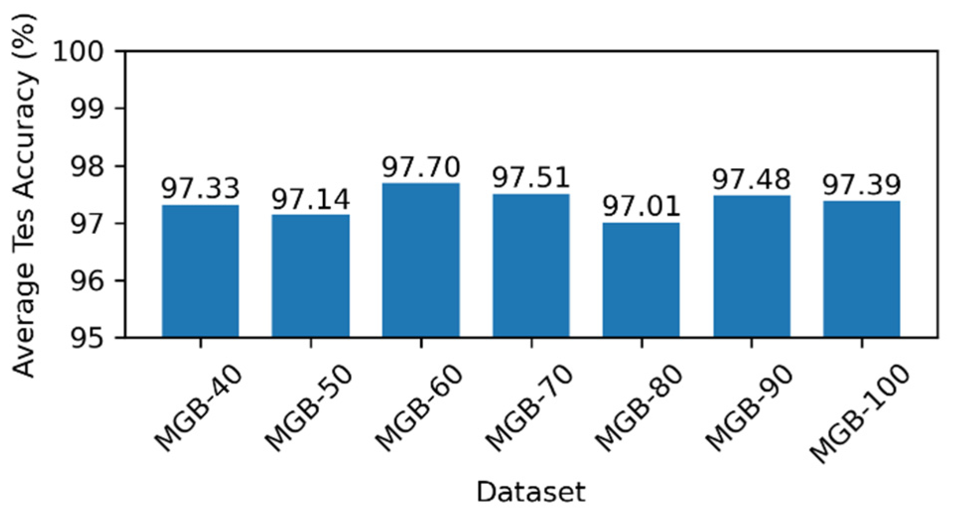
(2)

The dataset generated by the filter bank, containing 60 filters as the input to the model, yields a maximum recognition accuracy of 97.7%. Adding more filters does not improve the recognition accuracy of the model.

(3)

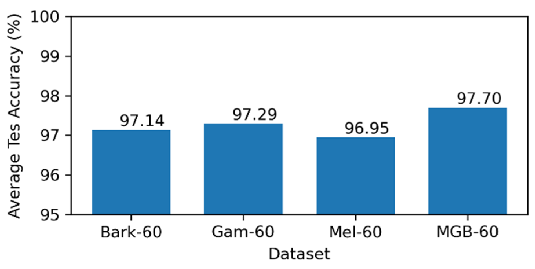
The multi-spectrogram fusion method for arc sound feature extraction increases the recognition accuracy of the weld penetration state to 97.7% (MGB-60), which is 0.56%, 0.41% and 0.75% higher than the recognition accuracy of the Mel spectrogram (Mel-60, 97.14%), GT spectrogram (GT-60, 97.29%) and Bark spectrogram (Bark-60, 96.95%), respectively.

(4)

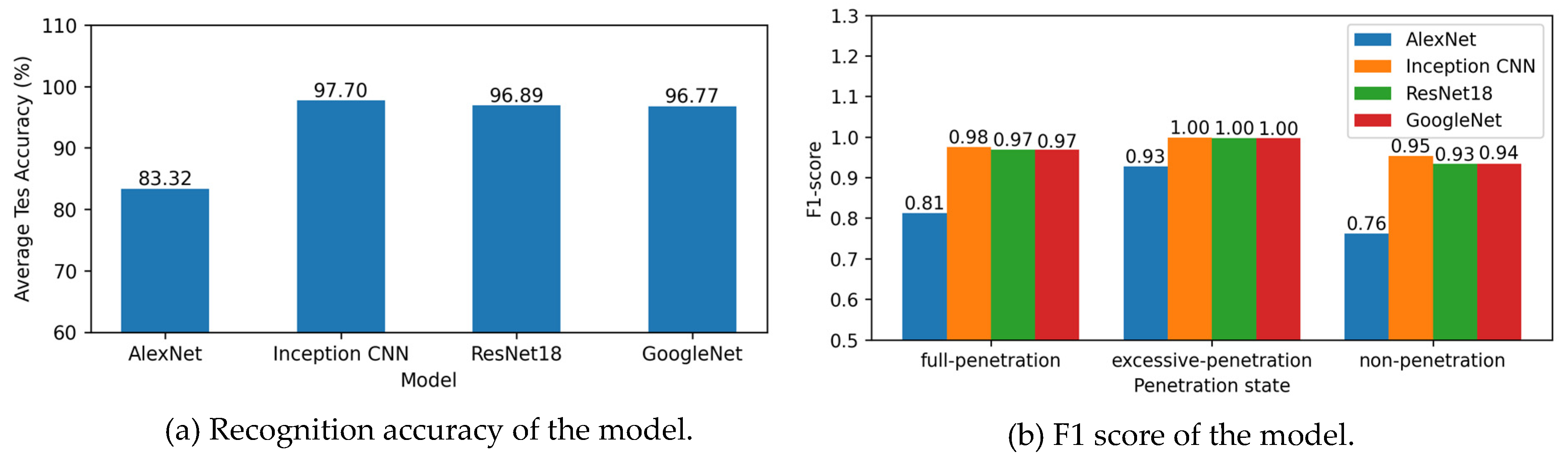
The recognition accuracy of Inception CNN, proposed in this paper, is 0.93% better than that of GoogleNet, and the recognition results are more stable. It also has better recognition results and greater stability compared to AlexNet and ResNet.

References

1. Selvi, S.; Vishvaksenan, A.; Rajasekar, E. Cold metal transfer (CMT) technology—An overview. Def. Technol. 2018, 14, 28–44. [Google Scholar] [CrossRef]
2. Pickin, C.G.; Williams, S.W.; Lunt, M. Characterisation of the cold Metal transfert (CMT) process and its application for low dilution cladding. J. Mater. Process. Technol. 2011, 211, 496–502. [Google Scholar] [CrossRef]
3. Furukawa, K. New CMT arc welding process—Welding of steel to aluminium dissimilar metals and welding of super-thin aluminium sheets. Weld. Int. 2006, 20, 440–445. [Google Scholar] [CrossRef]
4. González, J.; Rodríguez, I.; Prado-Cerqueira, J.L.; Diéguez, J.L.; Pereira, A. Additive manufacturing with GMAW welding and CMT technology. Procedia Manuf. 2017, 13, 840–847. [Google Scholar] [CrossRef]
5. Derekar, K.S.; Addison, A.; Joshi, S.S.; Zhang, X.; Lawrence, J.; Xu, L.; Melton, G.; Griffiths, D. Effect of pulsed metal inert gas (pulsed-MIG) and cold metal transfer (CMT) techniques on hydrogen dissolution in wire arc additive manufacturing (WAAM) of aluminium. Int. J. Adv. Manuf. Technol. 2020, 107, 311–331. [Google Scholar] [CrossRef]
6. Ji, T.; Nor, N.M. Deep Learning-Empowered Digital Twin Using Acoustic Signal for Welding Quality Inspection. Sensors 2023, 23, 2643. [Google Scholar] [CrossRef] [PubMed]
7. Wang, Q.; Gao, Y.; Huang, L.; Gong, Y.; Xiao, J. Weld bead penetration state recognition in GMAW process based on a central auditory perception model. Measurement 2019, 147, 106901. [Google Scholar] [CrossRef]
8. Wu, J.; Shi, J.; Gao, Y.; Gai, S. Penetration Recognition in GTAW Welding Based on Time and Spectrum Images of Arc Sound Using Deep Learning Method. Metals 2022, 12, 1549. [Google Scholar] [CrossRef]
9. Gao, Y.; Wang, Q.; Xiao, J.; Zhang, H. Penetration state identification of lap joints in gas tungsten arc welding process based on two channel arc sounds. J. Mater. Process. Technol. 2020, 285, 116762. [Google Scholar] [CrossRef]
10. Cui, Y.; Shi, Y.; Hong, X. Analysis of the frequency features of arc voltage and its application to the recognition of welding penetration in K-TIG welding. J. Manuf. Process. 2019, 46, 225–233. [Google Scholar] [CrossRef]
11. Cui, Y.; Shi, Y.; Zhu, T.; Cui, S. Welding penetration recognition based on arc sound and electrical signals in K-TIG welding. Meas. Measurement 2020, 163, 107966. [Google Scholar] [CrossRef]
12. Lu, J.; Xie, H.; Chen, X.; Han, J.; Bai, L.; Zhao, Z. Online welding quality diagnosis based on molten pool behavior prediction. Opt. Laser Technol. 2020, 126, 106126. [Google Scholar] [CrossRef]
13. Lu, J.; He, H.; Shi, Y.; Bai, L.; Zhao, Z.; Han, J. Quantitative prediction for weld reinforcement in arc welding additive manufacturing based on molten pool image and deep residual network. Addit. Manuf. 2021, 41, 101980. [Google Scholar] [CrossRef]
14. Lv, N.; Xu, Y.; Li, S.; Yu, X.; Chen, S. Automated control of welding penetration based on audio sensing technology. J. Mater. Process. Technol. 2017, 250, 81–98. [Google Scholar] [CrossRef]
15. Zhao, Z.; Lv, N.; Xiao, R.; Liu, Q.; Chen, S. Recognition of penetration states based on arc sound of interest using VGG-SE network during pulsed GTAW process. J. Manuf. Process. 2023, 87, 81–96. [Google Scholar] [CrossRef]
16. Ren, W.; Wen, G.; Xu, B.; Zhang, Z. A Novel Convolutional Neural Network Based on Time-Frequency Spectrogram of Arc Sound and Its Application on GTAW Penetration Classification. IEEE Trans. Ind. Inform. 2021, 17, 809–819. [Google Scholar] [CrossRef]
17. Liu, L.; Chen, H.; Chen, S. Quality analysis of CMT lap welding based on welding electronic parameters and welding sound. J. Manuf. Process. 2022, 74, 1–13. [Google Scholar] [CrossRef]
18. Yang, G.; Guan, K.; Zou, L.; Sun, Y.; Yang, X. Weld Defect Detection of a CMT Arc-Welded Aluminum Alloy Sheet Based on Arc Sound Signal Processing. Appl. Sci. 2023, 13, 5152. [Google Scholar] [CrossRef]
19. Salvati, D.; Drioli, C.; Foresti, G.L. A late fusion deep neural network for robust speaker identification using raw waveforms and gammatone cepstral coefficients. Expert Syst. Appl. 2023, 222, 119750. [Google Scholar] [CrossRef]
20. Liang, R.; Kong, F.; Xie, Y.; Tang, G.; Cheng, J. Real-Time Speech Enhancement Algorithm Based on Attention LSTM. IEEE Access 2020, 8, 48464–48476. [Google Scholar] [CrossRef]
21. Ancilin, J.; Milton, A. Improved speech emotion recognition with Mel frequency magnitude coefficient. Appl. Acoust. 2021, 179, 108046. [Google Scholar] [CrossRef]
22. Szegedy, C.; Liu, W.; Jia, Y.; Sermanet, P.; Reed, S.; Anguelov, D.; Erhan, D.; Vanhoucke, V.; Rabinovich, A.; Liu, W.; et al. Going deeper with convolutions. In Proceedings of the 2015 IEEE Conference on Computer Vision and Pattern Recognition (CVPR), Boston, MA, USA, 7–12 June 2015; pp. 1–9. [Google Scholar] [CrossRef]
23. Li, J.; Song, G.; Zhang, M. Occluded offline handwritten Chinese character recognition using deep convolutional generative adversarial network and improved GoogLeNet. Neural Comput. Appl. 2020, 32, 4805–4819. [Google Scholar] [CrossRef]
24. Mondal, S.; Barman, A.D. Speech activity detection using time-frequency auditory spectral pattern. Appl. Acoust. 2020, 167, 107403. [Google Scholar] [CrossRef]
25. Liu, S.; Li, R.; Li, Q.; Zhao, J. Porn streamer audio recognition based on deep learning and random Forest. Appl. Intell. 2023, 53, 18857–18867. [Google Scholar] [CrossRef]
26. Malayath, N.; Hermansky, H. Data-driven spectral basis functions for automatic speech recognition. Speech Commun. 2003, 40, 449–466. [Google Scholar] [CrossRef]
27. Toyoshima, I.; Okada, Y.; Ishimaru, M.; Uchiyama, R.; Tada, M. Multi-Input Speech Emotion Recognition Model Using Mel Spectrogram and GeMAPS. Sensors 2023, 23, 1743. [Google Scholar] [CrossRef] [PubMed]
28. Tao, H.; Wang, P.; Chen, Y.; Stojanovic, V.; Yang, H. An unsupervised fault diagnosis method for rolling bearing using STFT and generative neural networks. J. Frankl. Inst. 2020, 357, 7286–7307. [Google Scholar] [CrossRef]
29. Nagarajan, S.; Nettimi, S.S.S.; Kumar, L.S.; Nath, M.K.; Kanhe, A. Speech emotion recognition using cepstral features extracted with novel triangular filter banks based on bark and ERB frequency scales. Digit. Signal Process. 2020, 104, 102763. [Google Scholar] [CrossRef]
30. Mondal, S.; Barman, A.D. Human auditory model based real-time smart home acoustic event monitoring. Multimed. Tools Appl. 2022, 81, 887–906. [Google Scholar] [CrossRef]
31. Hermansky, H. Perceptual linear predictive (PLP) analysis of speech. J. Acoust. Soc. Am. 1990, 87, 1738–1752. [Google Scholar] [CrossRef]
32. Zhang, Z.; Wen, G.; Chen, S. Weld image deep learning-based on-line defects detection using convolutional neural networks for Al alloy in robotic arc welding. J. Manuf. Process. 2019, 45, 208–216. [Google Scholar] [CrossRef]
33. Wu, D.; Huang, Y.; Zhang, P.; Yu, Z.; Chen, H.; Chen, S. Visual-Acoustic Penetration Recognition in Variable Polarity Plasma Arc Welding Process Using Hybrid Deep Learning Approach. IEEE Access 2020, 8, 120417–120428. [Google Scholar] [CrossRef]
34. Ma, G.; Yu, L.; Yuan, H.; Xiao, W.; He, Y. A vision-based method for lap weld defects monitoring of galvanized steel sheets using convolutional neural network. J. Manuf. Process. 2021, 64, 130–139. [Google Scholar] [CrossRef]
35. Gaba, S.; Budhiraja, I.; Kumar, V.; Garg, S.; Kaddoum, G.; Hassan, M.M. A federated calibration scheme for convolutional neural networks: Models, applications and challenges. Comput. Commun. 2022, 192, 144–162. [Google Scholar] [CrossRef]
36. Zhang, Q.; Zhang, M.; Chen, T.; Sun, Z.; Ma, Y.; Yu, B. Recent advances in convolutional neural network acceleration. Neurocomputing 2019, 323, 37–51. [Google Scholar] [CrossRef]
37. Ioffe, S.; Szegedy, C. Batch normalization: Accelerating deep network training by reducing internal covariate shift. In Proceedings of the 32nd International Conference on Machine Learning, Lille, France, 6–11 July 2015; Volume 1, pp. 448–456. [Google Scholar]
38. Reyad, M.; Sarhan, A.M.; Arafa, M. A modified Adam algorithm for deep neural network optimization. Neural Comput. Applic 2023, 35, 17095–17112. [Google Scholar] [CrossRef]
Figure 1. Flowchart of the proposed method.
Electronics 12 04910 g001
Figure 2. Extraction of MGB spectrum.
Electronics 12 04910 g002
Figure 3. Components of customized Inception CNN architecture.
Electronics 12 04910 g003
Figure 4. Experimental setup.
Electronics 12 04910 g004
Figure 5. Weld seam penetration status and arc acoustic signals.
Electronics 12 04910 g005
Figure 6. Arc sound frequency domain signal.
Electronics 12 04910 g006
Figure 7. Comparison of frequency band energies of arc sound signals.
Electronics 12 04910 g007
Figure 8. Comparison of average test accuracies for different datasets.
Electronics 12 04910 g008
Figure 9. Comparison of sound spectrograms.
Electronics 12 04910 g009
Figure 10. Comparison of average test accuracy between single-spectrogram datasets and multilingual spectrogram fusion dataset.
Electronics 12 04910 g010
Figure 11. Model comparison.
Electronics 12 04910 g011