Self-Tuning Process Noise in Variational Bayesian Adaptive Kalman Filter for Target Tracking

Abstract

Many practical systems, such as target tracking, navigation systems, autonomous vehicles, and other applications, are usually applied in dynamic conditions. Thus, the actual noise statistics characteristics of these systems are generally time varying and unknown, which will deteriorate the state estimation accuracy of the Kalman filter (KF) and even cause filter diverging. To address this issue, this paper proposes an adaptive process noise covariance (Q_k)-based variational Bayesian adaptive Kalman filter (AQ-VBAKF) algorithm. Firstly, the adaptive factor is introduced to self-tune the process noise covariance; the adaptive factor is obtained based on the innovation sequences, which can adapt to the input measurement values. Then, the VB solution is applied to approximate the time variant and unknown measurement noise covariance. Therefore, this proposed algorithm can adjust the process noise covariance and the measurement noise covariance simultaneously based on the variable input signals, which can improve the self-adaptive ability of the state estimation filter in dynamic conditions. According to the dynamic target tracking test results, the proposed AQ-VBAKF outperforms several other existing filtering methods in estimation accuracy, robustness, and computational efficiency.

1. Introduction

In many practical applications, such as target tracking, positioning, autonomous vehicles, and so on, state estimation has been widely deployed [1,2,3,4]. The KF (Kalman filter) can obtain the optimal estimation for the minimum mean square error (MMSE) if the noise covariances are accurate under the linear Gaussian condition [5]. In the KF iteration, noise covariances are preselected and kept constant throughout the whole filtering process. However, when the practical systems work in dynamic environments, the constant noise covariances cannot reflect the real dynamic circumstances. For example, autonomous vehicle systems [6] inherently work in dynamic environments, where the sensor measurement, environment conditions, and vehicle dynamics are time varying and difficult to obtain. In this condition, the accurate noise statistics of practical systems are usually unknown. The actual noise covariances vary with the changes in environments. Thus, constant noise covariances for KF may degrade the filtering performance in dynamic conditions. Therefore, advanced estimation methods are necessary for autonomous vehicle systems, target tracking systems, and other applications.

Accordingly, to address this issue, several adaptive KF (AKF) methods have been developed. The AKF algorithms include the multiple mode AKF [7], the Sage-Husa AKF [8], the fading AKF [9], and the variational Bayesian-based AKF (VBAKF) [10]. The multiple mode AKF requires a bank of KFs operating simultaneously, resulting in a large computational burden. The Sage-Husa AKF uses the covariance matching method to estimate the maximum posterior noise, which cannot ensure that it will converge to the accurate noise covariances. The fading AKF introduces the fading factor to decrease the weight of the current measurement value. However, the fading AKF usually needs multiple fading factors, which are not easy to calculate [11].

The variational Bayesian-based AKF (VBAKF) has been widely utilized, as it can use a factorized free-form distribution to approximate the unknown measurement noise covariance matrix (MNCM) and the state vector’s joint posterior distribution [12,13]. However, in the VBAKF algorithm, the process noise covariance matrix (PNCM) is predefined and kept constant, which cannot reflect the actual noise environment and, thus, will deteriorate the filtering performance in time-varying situations. Huang et al. [14] proposed the VBAKF-PR algorithm to estimate the online MNCM and the predicted state error covariance matrix together, and more accurate results were obtained. However, the VBAKF-PR approach needs a predefined PNCM and has a large computational burden. In reference [15], the predicted state error covariance matrix was estimated, but the PNCM stayed constant. In reference [16], to overcome the issue that the PNCM’s distribution and the system state vector’s distribution are non-conjugate, black-box variational inference was used to solve this problem. In [17], a sliding window variational AKF was proposed, which relies on approximating the smoothing posterior distribution. However, these algorithms either have a high computational burden or the PNCM stays constant, which will decrease the filtering performance in dynamic conditions. Since the inaccurate predefined PNCM is used for each iteration, this may cause a decline in estimation accuracy.

To enhance the VBAKF’s performance in dynamic systems, an adaptive PNCM ($Q_k$)-based variational Bayesian adaptive KF (AQ-VBAKF) method is proposed in this paper. The main contributions of this paper are as follows:

• To further improve the VBAKF algorithm in dynamic systems and to improve the adaptability of PNCM, the proposed AQ-VBAKF algorithm can not only estimate the MNCM online, but can also self-tune the PNCM in real time. Therefore, the AQ-VBAKF can adapt to the input variable signals in the linear dynamic system.
• The VBAKF algorithm can only estimate the MNCM, but the PNCM stays constant during the whole filtering process, which will decrease the filtering performance. In the proposed algorithm, the adaptive factor is introduced to tune the PNCM in real time, meaning the fixed PNCM does not cause a decline in the VBAKF estimation accuracy at each iteration.
• The proposed algorithm is evaluated using the target tracking simulation. Based on a series of experiments, the proposed AQ-VBAKF can improve the filtering accuracy and robustness in comparison with other filtering methods under dynamic conditions. Moreover, the computational burden is not heavy, thus it can be applied in practical systems.

The structure of the paper is summarized as follows. The state-space model and problem statement are described in Section 2. The proposed AQ-VBAKF approach is illustrated in Section 3. The AQ-VBAKF method is verified by target tracking tests in Section 4. The conclusions are drawn in Section 5.

2. State-Space Model and Problem Statement

For the linear Gaussian discrete-time system, the state-space model is demonstrated as follows:

$${\mathbf{x}}_k=F_k{\mathbf{x}}_{k-1}+{\mathsf{\omega }}_{k-1}$$

(1)

$$z_k=H_k{\mathbf{x}}_k+{\mathsf{\upsilon }}_k$$

(2)

where Equation (1) denotes the system model, and Equation (2) denotes the measurement model. $k\in \mathbb{N}$ represents the sampling time point. ${\mathbf{x}}_k\in {ℝ}^{n_x}$ and ${\mathbf{z}}_k\in {ℝ}^{n_z}$ denote the state vector with $n_x$ dimensions and the measurement vector with $n_z$ dimensions at the k-th epoch, respectively. $F_k$ and $H_k$ are the system transition matrix and the observation matrix at the k-th epoch. The dimensions of $F_k$ and $H_k$ are $n_x\times n_x$ and $n_z\times n_x$, respectively. ${\mathsf{\omega }}_{k-1}$ is the process noise that obeys $\mathrm{N}(0, Q_{k-1})$. ${\mathsf{\upsilon }}_k$ represents the measurement noise that obeys $\mathrm{N}(0, R_k)$. The dimensions of $Q_{k-1}$ and $R_k$ are $n_x\times n_x$ and $n_z\times n_z$, respectively.

The KF algorithm includes two procedures, which are the prediction process and the correction process. The prediction procedure is expressed as [18]:

$${\widehat{x}}_{k|k-1}^{}=F_k{\widehat{x}}_{k-1|k-1}^{}$$

(3)

$$P_{k|k-1}^{}=F_k{P}_{k-1|k-1}^{}{F}_k^{\mathrm{T}}+Q_{k-1}$$

(4)

Then, the correction process is defined as [18]:

$$K_k=P_{k|k-1}^{}{H}_k^{\mathrm{T}}{\left(H_k{P}_{k|k-1}^{}{H}_k^{\mathrm{T}}+R_{k-1}\right)}^{-1}$$

(5)

$${\widehat{x}}_{k|k}^{}={\widehat{x}}_{k|k-1}^{}+K_k\left(z_k-H_k{\widehat{x}}_{k|k-1}^{}\right)$$

(6)

$$P_{k|k}^{}=P_{k|k-1}^{}-K_k{H}_k{P}_{k|k-1}^{}$$

(7)

where $K_k$ is the KF gain. The dimension of $K_k$ is $n_x\times n_z$. ${\widehat{x}}_{k|k-1}^{}$ and ${\widehat{x}}_{k-1|k-1}^{}$ represent the predicted and estimated state values. $P_{k|k-1}^{}$ and $P_{k-1|k-1}^{}$ represent the predicted and estimated state error covariance matrices.

In dynamic conditions, such as integration navigation systems, target tracking systems, and autonomous vehicles, the actual noise covariances vary with the changes in environments and the accurate noise statistics of practical systems are usually unknown. The inaccurate and constant noise covariances $Q_k$ and $R_k$ in the KF may cause suboptimal estimations and even divergence. Therefore, an adaptive KF algorithm for the inaccurate noise covariance matrices is necessary under practical dynamic conditions. Accordingly, a novel AQ-VBAKF approach is proposed to self-tune the variable and unknown MNCM and PNCM under dynamic conditions.

3. Proposed AQ-VBAKF Algorithm

3.1. Variational Bayesian Approximation for MNCM ($R_k$)

According to Equations (1) and (2), the probability form for the state-space model is [19]:

$$p(z_k|{\mathbf{x}}_k,R_k)=\mathrm{N}(z_k|H_k{\mathbf{x}}_k,R_k)$$

(8)

where $\mathrm{N}(\cdot |\mu , \Sigma )$ represents the multivariate Gaussian distribution with a mean vector $\mu$ and covariance matrix $\Sigma$. Because $R_k$ is unknown, the VB algorithm is applied to acquire the posterior distribution $p({\mathbf{x}}_k,R_k|z_{1:k})$. However, it is usually not analytical to handle [12]. The approximation scheme VB is used to approximate the intractable posterior inference in the Bayesian model [12].

In linear and Gaussian systems, ${\mathbf{x}}_k$ is considered to be independent of the NCM. The joint distribution at the (k−1)-th epoch $p({\mathbf{x}}_k,R_k|z_{1:k-1})$ is decomposed as:

$$p({\mathbf{x}}_k,R_k|z_{1:k-1})=p({\mathbf{x}}_k|z_{1:k-1})p(R_k|z_{1:k-1})$$

(9)

$p({\mathbf{x}}_k|z_{1:k-1})$ is assumed as the Gaussian distribution, and $p(R_k|z_{1:k-1})$ can be considered as an inverse Wishart (IW) distribution, which is expressed as [16]:

$$p(x_k|z_{1:k-1})=\mathrm{N}(x_k|{\widehat{x}}_{k|k-1}^{},P_{k|k-1}^{})$$

(10)

$$p(R_k|z_{1:k-1})=\mathrm{IW}(R_k|{\widehat{v}}_{k|k-1},{\widehat{V}}_{k|k-1})$$

(11)

where $\mathrm{IW}(\cdot |w,W)$ represents the IW distribution. $w$ denotes the degrees of freedom’s number. $W$ represents the inverse scale matrix.

Employing the VB inference, the joint posterior distribution can be approximated as:

$$p({\mathbf{x}}_k,R_k|z_{1:k})\approx q({\mathbf{x}}_k)q(R_k)$$

(12)

where $q(\cdot )$ is the approximation for $p(\cdot )$. $q({\mathbf{x}}_k)$ and $q(R_k)$ are obtained based on the minimization of the Kullback-Leibler (KL) divergence between the real posterior distribution $p({\mathbf{x}}_k,R_k|z_{1:k})$ and the approximation $q({\mathbf{x}}_k)q(R_k)$, which is:

$$\begin{array}{ll}q({\mathbf{x}}_k)q(R_k)& =\arg \min \left\{\mathrm{KL}\left(q({\mathbf{x}}_k)q(R_k)\left|\right|p({\mathbf{x}}_k,R_k|z_{1:k})\right)\right\} \\ & =\arg \min \left\{{\displaystyle \int q({\mathbf{x}}_k)q(R_k)\log \left(\frac{q({\mathbf{x}}_k)q(R_k)}{p({\mathbf{x}}_k,R_k|z_{1:k})}\right)}d{\mathbf{x}}_{k}d{R}_k\right\}\end{array}$$

(13)

where $\mathrm{KL}(\mathrm{m}\left(x\left)\right||\mathrm{n}\right(x\left)\right)$ represents the KL divergence between m(x) and n(x).

The optimal solution of Equation (13) can be obtained as follows [20]:

$$\log q(R_k)=\underset{{\mathbf{x}}_k}{\mathrm{E}}[\log p({\mathbf{x}}_k,R_k,z_{1:k})]+C_{R_k}$$

(14)

$$\log q({\mathbf{x}}_k)=\underset{R_k}{\mathrm{E}}[\log p({\mathbf{x}}_k,R_k,z_{1:k})]+C_{{\mathbf{x}}_k}$$

(15)

where E[·] represents the expectation operator. $C_{R_k}$ and $C_{{\mathbf{x}}_k}$ denote the constants independent of $R_k$ and ${\mathbf{x}}_k$, respectively.

Because of the Bayesian rule, it can be given that:

$$\log p({\mathbf{x}}_k,R_k,z_{1:k})=\log p({\mathbf{x}}_k,R_k,z_k|z_{1:k-1})+\log p(z_{1:k-1})$$

(16)

Due to $p(z_{1:k-1})$ being independent of $R_k$ and ${\mathbf{x}}_k$, then:

$$\log p({\mathbf{x}}_k,R_k,z_{1:k})\propto \log p({\mathbf{x}}_k,R_k,z_k|z_{1:k-1})$$

(17)

Based on Equations (8), (10), and (11), $p({\mathbf{x}}_k,R_k,z_k|z_{1:k-1})$ is decomposed as [21]:

$$\begin{array}{l}p({\mathbf{x}}_k,R_k,z_k|z_{1:k-1})\\ =p(z_k|{\mathbf{x}}_k,R_k)p({\mathbf{x}}_k|R_k,z_{1:k-1})p(R_k|z_{1:k-1})\\ =\mathrm{N}(z_k|H_k{\mathbf{x}}_k,R_k)\mathrm{N}(x_k|{\widehat{x}}_{k|k-1}^{},P_{k|k-1}^{}\left)\mathrm{IW}\right(R_k|{\widehat{v}}_{k|k-1},{\widehat{V}}_{k|k-1})\end{array}$$

(18)

Accordingly, we can have:

$$\begin{array}{l}\log p({\mathbf{x}}_k,R_k,z_k|z_{1:k-1})=\\ -0.5{(z_k-H_k{\mathbf{x}}_k)}^{\mathrm{T}}{R}_k{}^{-1}(z_k-H_k{\mathbf{x}}_k)\\ -0.5{({\mathbf{x}}_k-{\widehat{x}}_{k|k-1}^{})}^{\mathrm{T}}{P}_{k|k-1}^{}{}^{-1}({\mathbf{x}}_k-{\widehat{x}}_{k|k-1}^{})\\ -0.5({\widehat{v}}_{k|k-1}+n_z+2)\log \left|R_k\right|-0.5\mathrm{tr}({\widehat{V}}_{k|k-1}{R}_k{}^{-1})+C\end{array}$$

(19)

where tr[·] denotes the matrix’s trace. $n_x$ and $n_z$ denote the dimensions of ${\mathbf{x}}_k$ and $z_k$, respectively. $C$ represents a constant independent of ${\mathbf{x}}_k$ and $R_k$.

Substituting Equations (17) and (19) into Equation (14), we can obtain the updated $q(R_k)$. $q(R_k)$ is approximated as the IW distribution:

$$q^{(s)}(R_k)=\mathrm{IW}(R_k|{\widehat{v}}_{k|k}^{(s)},{\widehat{V}}_{k|k}^{(s)})$$

(20)

where

$${\widehat{v}}_{k|k}^{(s)}={\widehat{v}}_{k|k-1}^{}+1$$

(21)

$${\widehat{V}}_{k|k}^{(s)}=N_k^{(s-1)}+{\widehat{V}}_{k|k-1}$$

(22)

$$N_k^{(s-1)}=(z_k-H_k{\widehat{\mathbf{x}}}_{k|k}^{(s-1)}){(z_k-H_k{\widehat{\mathbf{x}}}_{k|k}^{(s-1)})}^{\mathrm{T}}+H_k{P}_{k|k}^{(s-1)}{H}_k^{\mathrm{T}}$$

(23)

The superscript s denotes the s-th VB iteration. The dimensions of ${\widehat{V}}_{k|k-1}$ is $n_z\times n_z$ and ${\widehat{v}}_{k|k-1}^{}$ is scalar.

Substituting Equations (17) and (19) into Equation (15), $q({\mathbf{x}}_k)$ is updated as:

$$q^{(s)}({\mathbf{x}}_k)=\mathrm{N}({\mathbf{x}}_k|{\widehat{\mathbf{x}}}_{k|k}^{(s)},P_{k|k}^{(s)})$$

(24)

where

$$K_k^{(s)}={\widehat{P}}_{k|k-1}^{(s)}{H}_k^{\mathrm{T}}{\left[H_k{\widehat{P}}_{k|k-1}^{(s)}{H}_k^{\mathrm{T}}+{\left({\mathrm{E}}^{(s)}[R_k^{-1}]\right)}^{-1}\right]}^{-1}$$

(25)

$${\widehat{\mathbf{x}}}_{k|k}^{(s)}={\widehat{\mathbf{x}}}_{k|k-1}+K_k^{(s)}(z_k-H_k{\widehat{\mathbf{x}}}_{k|k-1})$$

(26)

$$P_{k|k}^{(s)}={\widehat{P}}_{k|k-1}^{(s)}-K_k^{(s)}{H}_k{\widehat{P}}_{k|k-1}^{(s)}$$

(27)

3.2. Adaptation of PNCM ($Q_k$)

In the VBAKF, the MNCM ($R_k$) is adjusted in real time. However, the PNCM ($Q_k$) stays constant in the filtering process. The constant $Q_k$ cannot match the actual noise statistic characteristic, so the adaptive method of $Q_k$ is proposed to enhance the estimation accuracy. Hence, the adaptive factor ${\lambda }_k$ is introduced to adjust $Q_k$, that is:

$$P_{k|k-1}^{}=F_k{P}_{k-1|k-1}^{}{F}_k^{\mathrm{T}}+{\lambda }_k{Q}_{k-1}$$

(28)

In the KF estimation, when the state estimations are accurate, the following equation is held [22]:

$$\begin{array}{l}\mathrm{E}[d_{k+j}{d}_k^{\mathrm{T}}]\approx \\ H_k{F}_k(I-K_{k+j-1}{H}_k) •F_k(I-K_{k+2}{H}_k)•F_k(P_{k|k-1}^{}{H}_k^{\mathrm{T}}-K_k{C}_k)j=1, 2\cdots \end{array}$$

(29)

where I represents the identity matrix and $d_k$ denotes innovation sequences, that is:

$$d_k={\mathbf{z}}_k-H_k{\widehat{\mathbf{x}}}_{k|k-1}^{}$$

(30)

where $C_k$ is the innovation covariance. The dimensions of $d_k$ and $C_k$ are $n_z\times 1$ and $n_z\times n_z$, respectively. To keep the estimation accurate, $\mathrm{E}[d_{k+j}{d}_k^{\mathrm{T}}]=0$ should be satisfied [22]. Therefore, according to Equation (29), $K_k$ should be selected to establish the following equation:

$$P_{k|k-1}^{}{H}_k^{\mathrm{T}}-K_k{C}_k=0$$

(31)

By substituting Equation (5) into Equation (31), it can be given that:

$$P_{k|k-1}^{}{H}_k^{\mathrm{T}}\left\{I-{\left(H_k{P}_{k|k-1}^{}{H}_k^{\mathrm{T}}+R_{k-1}\right)}^{-1}{C}_k\right\}=0$$

(32)

To satisfy Equation (32), the following equation should be held:

$$H_k{P}_{k|k-1}^{}{H}_k^{\mathrm{T}}+R_{k-1}=C_k$$

(33)

Because of Equation (28), then it can then be determined that:

$$C_k=H_k{F}_k{P}_{k-1|k-1}^{}{F}_k^{\mathrm{T}}{H}_k^{\mathrm{T}}+R_{k-1}+{\lambda }_k{H}_k{Q}_{k-1}{H}_k^{\mathrm{T}}$$

(34)

Therefore, the adaptive factor ${\lambda }_k$ can be obtained as:

$${\lambda }_k=\frac{\mathrm{tr}(C_k-H_k{F}_k{P}_{k-1|k-1}^{}{F}_k^{\mathrm{T}}{H}_k^{\mathrm{T}}-R_{k-1})}{\mathrm{tr}(H_k{Q}_{k-1}{H}_k^{\mathrm{T}})}$$

(35)

To keep the whole filtering process stable, the adaptive factor ${\lambda }_k$ should be larger than 1; that is:

$${\lambda }_k=\max \left(1,{\lambda }_k\right)$$

(36)

When the system experiences sudden changes, and the adaptive factor is larger than 1, then the corresponding Kalman gain will become larger based on Equation (5). Therefore, according to Equation (6), more weight will be added to the current measurement data and less weight will be given to the past state information, and then the state estimation will be more accurate. Therefore, ${\lambda }_k$ is obtained with:

$${\lambda }_k=\left\{\begin{array}{ll}\frac{\mathrm{tr}(C_k-H_k{F}_k{P}_{k-1|k-1}^{}{F}_k^{\mathrm{T}}{H}_k^{\mathrm{T}}-R_{k-1})}{\mathrm{tr}(H_k{Q}_{k-1}{H}_k^{\mathrm{T}})}& {\lambda }_k\ge 1\\ 1& {\lambda }_k<1\end{array}\right.$$

(37)

The innovation covariance $C_k$ is defined as:

$$C_k=\mathrm{E}[d_k{d}_k^T]$$

(38)

In general, it is difficult to obtain the actual innovation covariance. Thus, we use the window function method to estimate the innovation covariance [23]:

$${\widehat{C}}_k={\widehat{C}}_{k-1}+\frac{1}{N}\left(d_k{d}_k^T-d_{k-N}{d}_{k-N}^T\right)$$

(39)

where ${\widehat{C}}_k$ denotes the estimated innovation covariance, and N > 1 represents the window size and is a scalar.

3.3. Proposed Algorithm

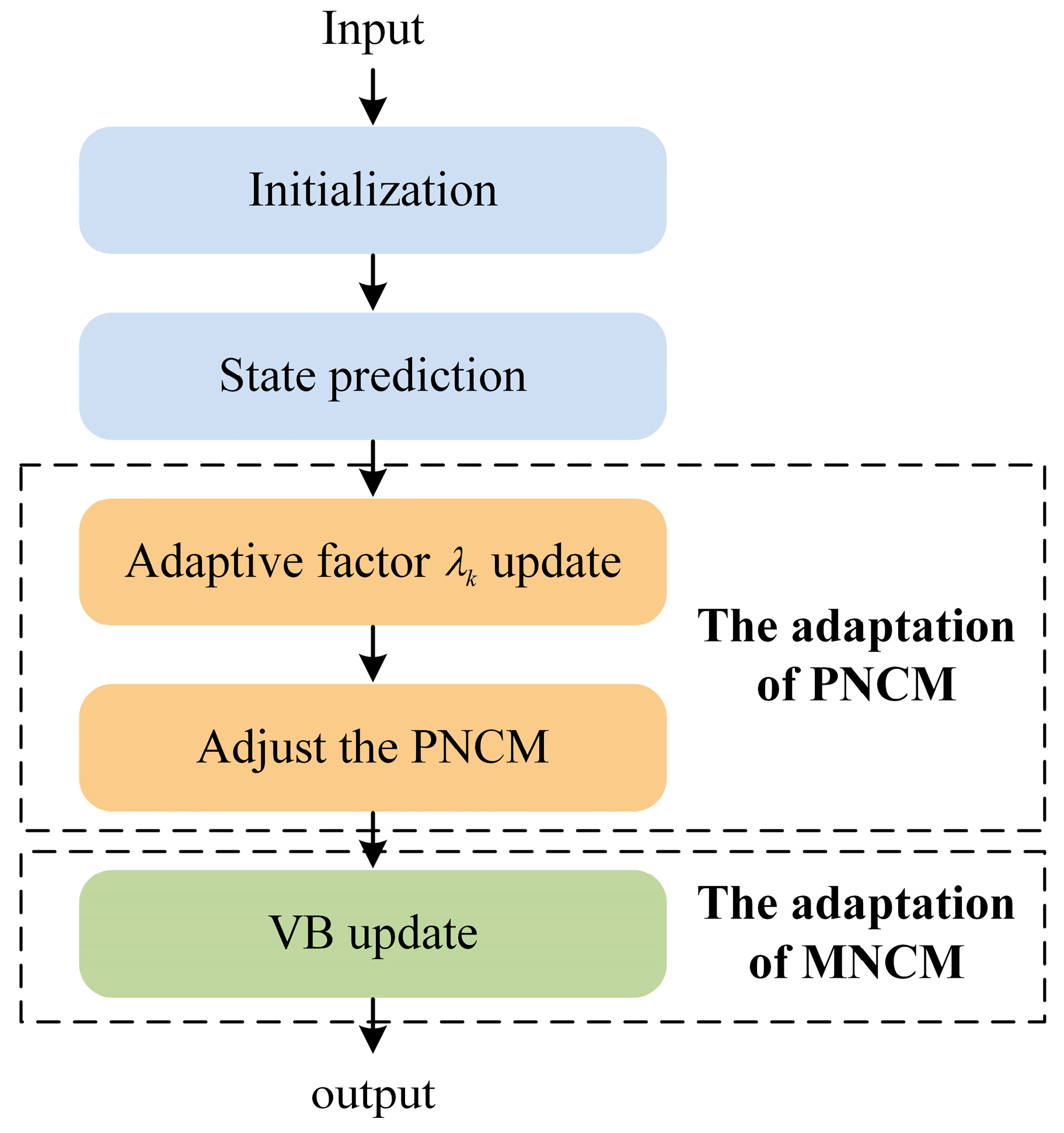
To summarize, the structure diagram of the proposed algorithm is shown in Figure 1. The detailed algorithm is demonstrated in Algorithm 1, where $\xi \in (0,1]$ represents the forgetting factor and S denotes the VB iteration number.

Algorithm 1: Proposed AQ-VBAKF Algorithm

Input: ${\widehat{\mathbf{x}}}_{k-1|k-1}^{}$, ${\mathbf{z}}_k$, $P_{k-1|k-1}^{}$, $R_{k-1}$, $Q_{k-1}$, ${\widehat{V}}_{k-1|k-1}$, ${\widehat{v}}_{k-1|k-1}$, $F_k$, $H_k$, N, $n_z$, S, $\xi$

Time update for state values: 1: ${\widehat{\mathbf{x}}}_{k|k-1}^{}$ can be obtained via Equation (3). The adaptive factor update and the time update for $P_{k|k-1}^{}$: 2: The adaptive factor is computed using Equations (30), (37), and (39). 3: $P_{k|k-1}^{}$ is obtained with Equation (28). VB estimation update: 4: Initialization: ${\widehat{P}}_{k|k-1}^{(0)}=P_{k|k-1}^{}$, ${\widehat{\mathbf{x}}}_{k|k-1}^{(0)}={\widehat{\mathbf{x}}}_{k|k-1}^{}$     ${\widehat{v}}_{k|k-1}=\xi ({\widehat{v}}_{k-1|k-1}-n_z-1)+n_z+1$, ${\widehat{V}}_{k|k-1}=\xi {\widehat{V}}_{k-1|k-1}$     For s = 1: S 5: Update $q^{(s)}(R_k)$ using Equations (21)–(23) 6: ${\left({\mathrm{E}}^{(s)}[R_k^{-1}]\right)}^{-1}$ is obtained with ${\left({\mathrm{E}}^{(s)}[R_k^{-1}]\right)}^{-1}={({\widehat{v}}_{k|k}^{(s)}-n_z-1)}^{-1}({\widehat{V}}_k^{(s)})$ 7: ${\widehat{\mathbf{x}}}_{k|k}^{(s)}$ and ${\widehat{P}}_{k|k}^{(s)}$ are obtained via Equations (25)–(27)     End Output: $P_{k|k}^{}$, ${\widehat{\mathbf{x}}}_{k|k}^{}$, ${\widehat{v}}_{k|k}^{}$, ${\widehat{V}}_{k|k}^{}$

4. Simulation Verification and Analysis

In this section, we adopt a target tracking test to assess the availability and superiority of the proposed AQ-VBAKF algorithm. The target tracking example’s state equation and measurement equation are:

$$x_k=\left[\begin{array}{cc}{I}_2& \Delta \sigma I_2\\ 0& I_2\end{array}\right]x_{k-1}+{\mathbf{n}}_{k-1}$$

(40)

$$z_k=\left[\begin{array}{cc}{I}_2& 0\end{array}\right]x_{k-1}+v_k$$

(41)

where $x_k={\left[\begin{array}{cccc}{\mathbf{x}}_k& y_k& {\dot{x}}_k& {\dot{y}}_k\end{array}\right]}^{\mathrm{T}}$ is the system state vector. Then, $(x_k,y_k)$ and $({\dot{x}}_k,{\dot{y}}_k)$ stand for the unknown positions and velocities. $\Delta \sigma$ is the sampling interval and $\Delta \sigma$ is set to 1 s. The true covariances of ${\mathbf{n}}_{k-1}$ and $v_k$ are described by:

$$Q_k=[0.5\cos (\frac{\mathsf{\pi }k}{T})+6.5]\left[\begin{array}{cc}\frac{\Delta {\sigma }^3}{3}{I}_2& 0.5\Delta {\sigma }^2{I}_2\\ 0.5\Delta {\sigma }^2{I}_2& \Delta \sigma I_2\end{array}\right]q$$

(42)

$$R_k=[0.05\cos (\frac{\mathsf{\pi }k}{T})+0.1]\left[\begin{array}{cc}1& 0.5\\ 0.5& 1\end{array}\right]r$$

(43)

where $I_2$ is a two-dimensional identity matrix. T denotes the simulation time and T = 1000 s. Additionally, $q$ is set as 1 m²/s³ and $r$ is set as 100 m². Moreover, the initial values for PNCM ($Q_0$) and MNCM ($R_0$) are set to $Q_0=\alpha I_4$ and $R_0=\beta I_2$.

4.1. Estimation Performance Analysis

To verify the filtering accuracy, we compare the proposed AQ-VBAKF with five other filtering estimation methods:

• KFTCM algorithm: the KF is iterated with true covariance matrices (KFTCM), which act as a reference.
• KFNCM algorithm: the KF is iterated with nominal covariance matrices (KFNCM), which are $Q_0$ and $R_0$. $Q_k$ and $R_k$ are fixed during the filtering process.
• AQKF algorithm: the KF is iterated with the adaptive $Q_k$; only $Q_k$ is adjusted based on the previous Section 3.2, and $R_k$ is fixed throughout the whole process.
• VBKF algorithm: $R_k$ is updated using the VB method and $Q_k$ is constant throughout the whole process.
• VBAKF-PR algorithm: the VBAKF-PR algorithm was demonstrated in [14].

In the simulation, the initial values are set to $P_{0|0}=\mathrm{diag}([100, 100, 100, 100])$ and $x_0{=[100, 100, 10, 10]}^{\mathrm{T}}$.

Table 1. Parameters settings for different algorithms.

Algorithms	α	β	ξ	S	N	τ
KFNCM	1	10	-	-	-	-
AQKF	1	10	-	-	5	-
VBAKF	1	10	0.99	15	-	-
VBAKF-PR	1	10	0.99	15	-	10
Proposed AQ-VBAKF	1	10	0.99	15	5	-

shows the different algorithms’ parameter settings. S is the VB iteration times. The iteration times should be proper to ensure the VB approximate converges to the optimal results. Generally, VB iteration times should be more than 6 to make the filter converge, thus S is chosen as 15 [24]. N represents the window size for the AQKF and AQ-VBAKF algorithms, which is analyzed in the simulation later. α and β are used for setting $Q_0=\alpha I_4$ and $R_0=\beta I_2$. In fact, the prior noise information of the system is usually unknown; thus, the setting of $Q_0$ and $R_0$ are usually not accurate. Moreover, α and β are both variables to test the robustness of the algorithms with different $Q_0$ and $R_0$ values. ξ is used for VB inference initialization, as shown in Algorithm 1, which should be $\xi \in (0,1]$ to ensure that the posterior and prior PDFs have the same forms. τ is used for the VBAKF-PR algorithm.

The RMSE (root mean square error) and ARMSE (average RMSE) are used to validate the state estimation accuracy based on the following formulas:

$${\mathrm{RMSE}}_{\mathrm{pos}}(j)\triangleq \sqrt{\frac{1}{M_{\mathrm{c}}}{\displaystyle \sum _{j=1}^{M_{\mathrm{c}}}\left[{(x_j^l-{\widehat{x}}_j^l)}^2-{(y_j^l-{\widehat{y}}_j^l)}^2\right]}}$$

(44)

$${\mathrm{ARMSE}}_{\mathrm{pos}}\triangleq \frac{1}{T}{\displaystyle \sum _{j=1}^T{\mathrm{RMSE}}_{\mathrm{pos}}(j)}$$

(45)

where $M_{\mathrm{c}}$ represents the Monte Carlo (MC) test number, and $M_{\mathrm{c}}$ = 1000. $(x_i^l,y_i^l)$ and $({\widehat{x}}_i^l,{\widehat{y}}_i^l)$ represent the true and the estimated positions at the l-th MC test, respectively. T is set to 1000 s. For velocity, the definitions of RMSE and ARMSE are similar.

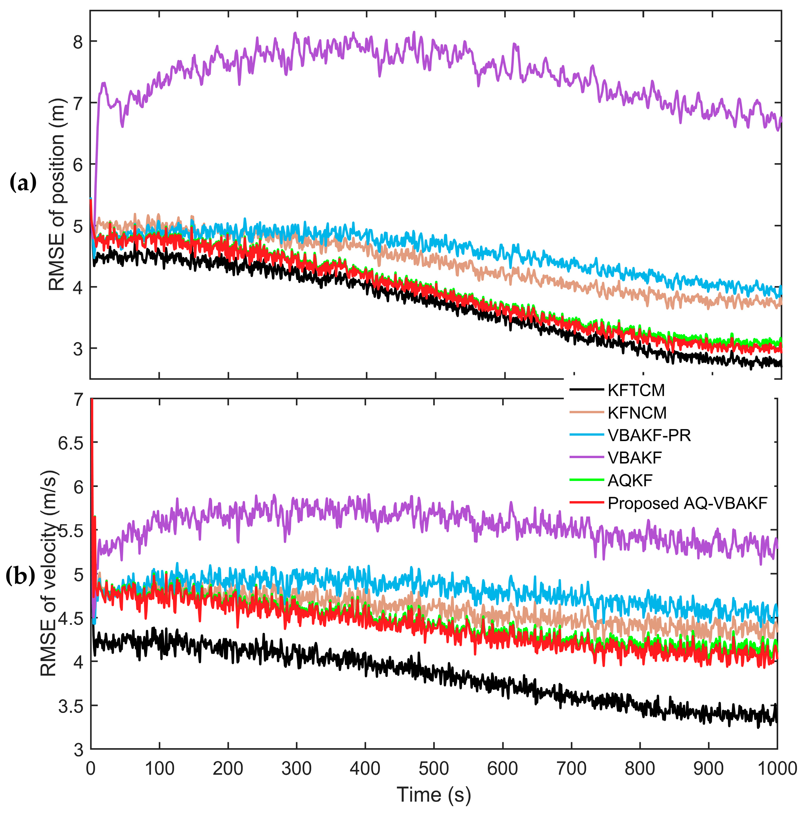
Figure 2 demonstrates the RMSEs for different algorithms, where the KFTCM has the smallest RMSEs, and acts as a reference. In comparison with the KFNCM, AQKF, VBAKF, and VBAKF-PR algorithms, the proposed AQ-VBAKF has the smallest RMSEs for position and velocity. The VBAKF has the worst performance, which indicates that the VBAKF is even worse than the KFNCM when the initial values are far away from the true values. The VBAKF cannot guarantee an optimal outcome in any case. Due to the adaptive predicted state error covariance matrix, the VBAKF-PR shows higher accuracy than the VBAKF, but is also worse than the KFNCM due to the initial value deviating from the true values. The AQKF is slighter worse than the proposed AQ-VBAKF since the AQKF lacks the ability to update the MNCM ($R_k$).

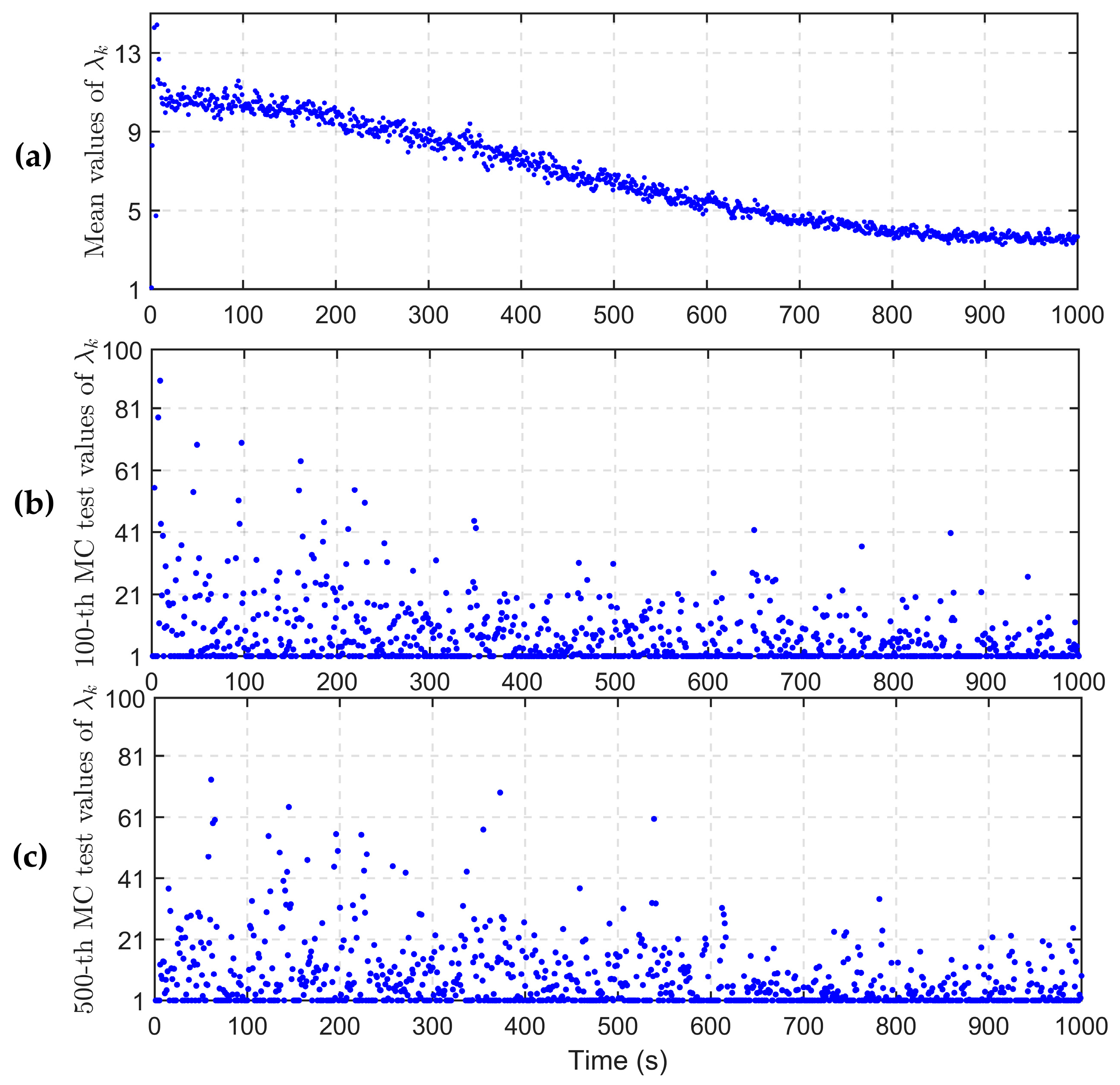
Figure 3a shows the mean values of ${\lambda }_k$ in the 1000 Monte Carlo (MC) tests based on the following formulas:

$${\lambda }_{\mathrm{mean}}(k)\triangleq \frac{1}{M_c}{\displaystyle \sum _{j=1}^{M_c}{\lambda }_j^{}(k)}$$

(46)

where $M_c=1000$, and k denotes the k-th epoch. Figure 3b,c show the 100th and 500th MC test values of ${\lambda }_k$, respectively. It can be shown that when the RMSEs of position and velocity are higher in Figure 2 for $k\in [0,500]$, the values of ${\lambda }_k$ are higher in Figure 3. This indicates that when the estimations of position and velocity deviate from the true values, the values of ${\lambda }_k$ will be larger to adjust the PNCM. Instead, when the estimations of position and velocity are close to the true values, the values of adaptive factor ${\lambda }_k$ will become smaller. This indicates that the adaptive factor ${\lambda }_k$ can adjust the PNCM according to the input signals.

4.2. Robustness Analysis for PNCM and MNCM Initial Value Settings

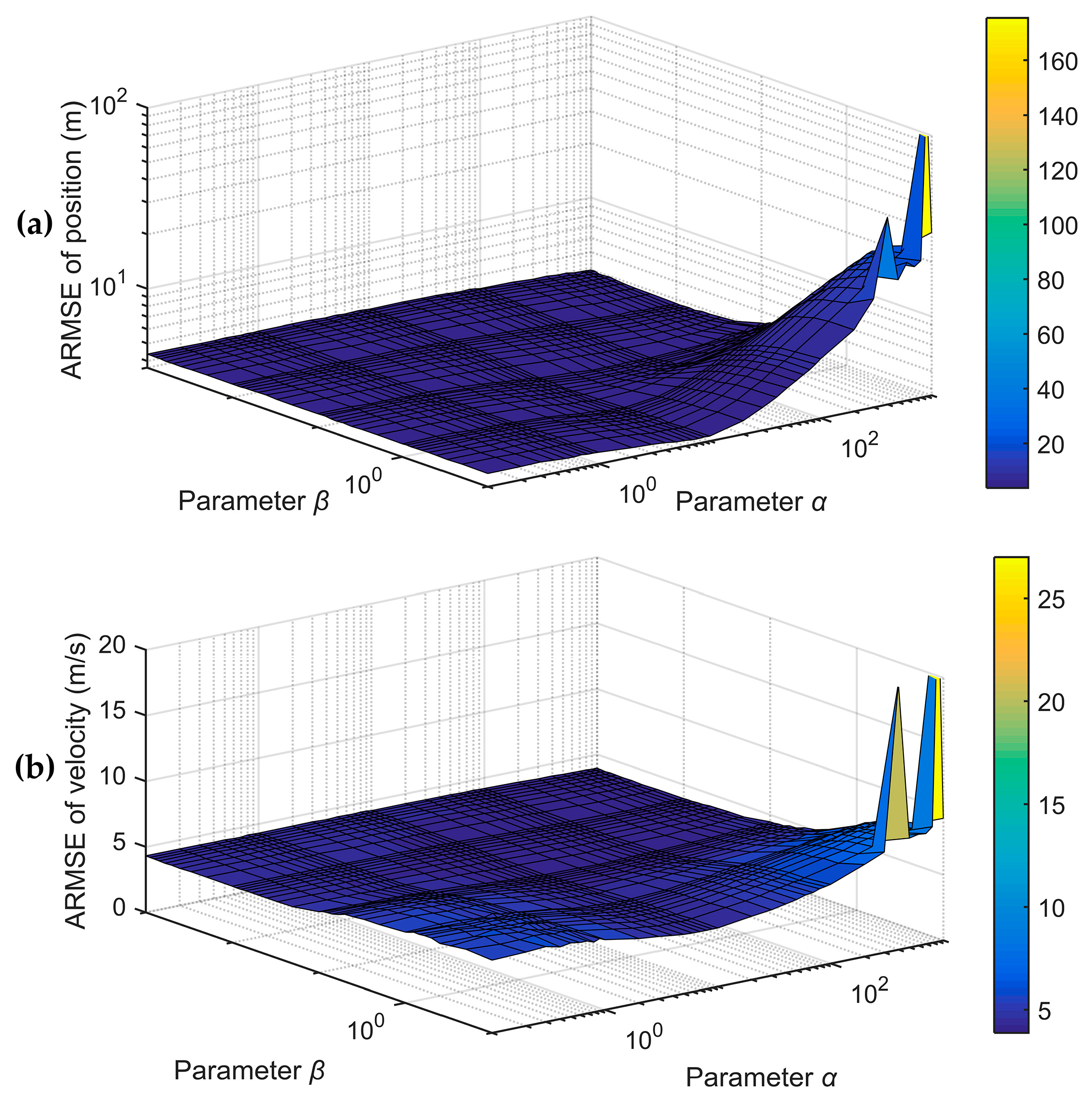
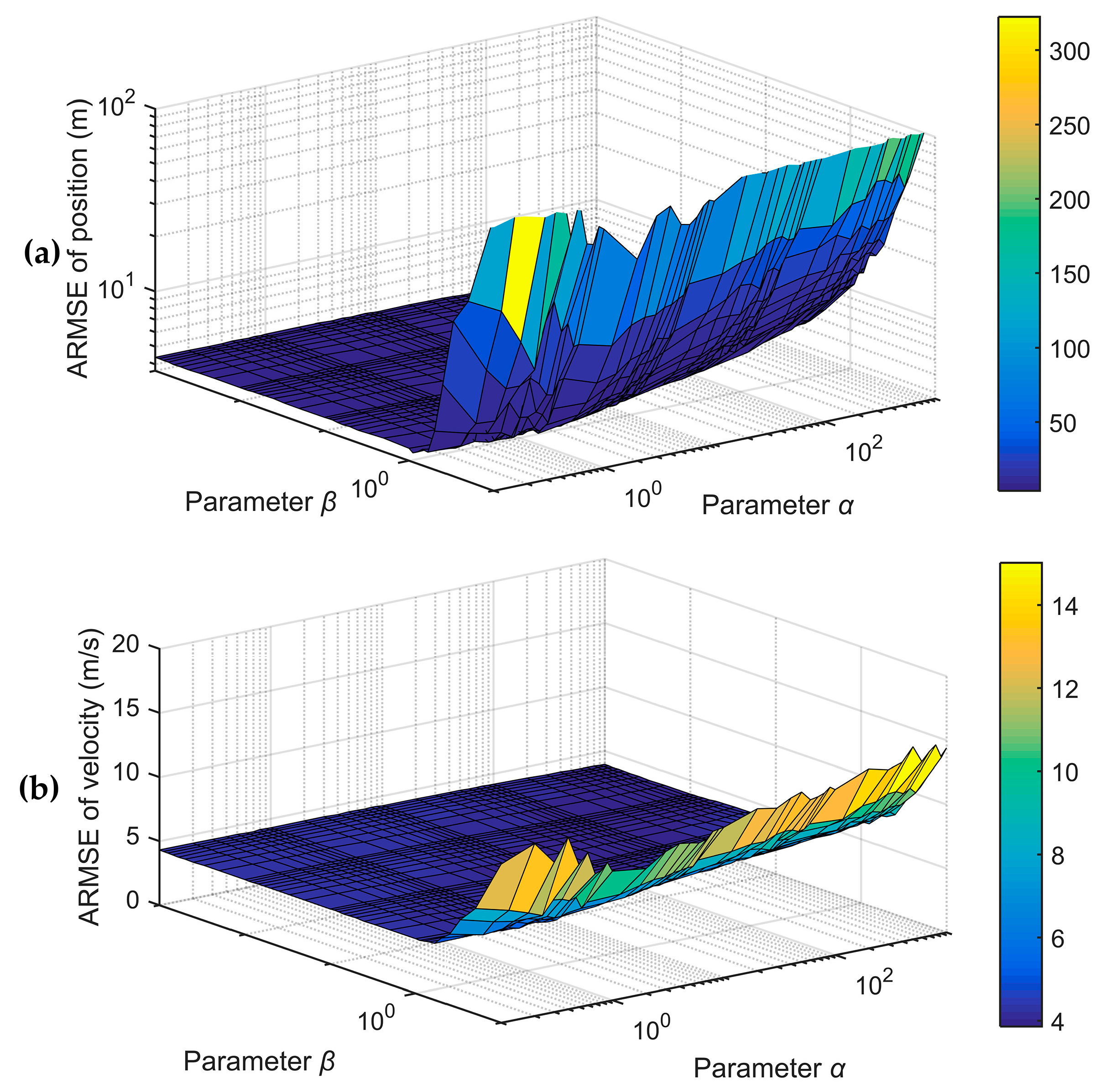
To assess the proposed AQ-VBAKF’s robustness, the ARMSEs of the AQ-VBAKF algorithm for different initial PNCM ($Q_0$) and MNCM ($R_0$) values were calculated and are presented in Figure 4. For comparison, Figure 5 demonstrates the ARMSEs for the VBAKF-PR. α and β are selected in the range of $(\alpha , \beta )\in [0.1, 1000]\times [0.1, 1000]$. To reduce the time consumption and keep the results reliable, $M_{\mathrm{c}}$ is set to 20. Moreover, Table 1 demonstrates other parameter settings, including ξ, S, N, and τ.

In Figure 4, as we can see, the ARMSEs for position and velocity stay small and stable in most cases. However, when the parameters are in the range of $(\alpha , \beta )\in [100, 1000]\times [0.1, 1]$, the ARMSEs for position and velocity increase, which indicates that the filtering estimations are not so accurate. Figure 5 shows the VBAKF-PR’s results. In the range of $(\alpha , \beta )\in [0.1, 1000]\times [0.1, 1]$, as the parameter β decreases, the ARMSEs increase. Therefore, the AQ-VBAKF is more robust than the VBAKF-PR in the range of $(\alpha , \beta )\in [0.1, 100]\times [0.1, 1]$, in which the initial values of the PNCM ($Q_0$) and MNCM ($R_0$) deviate from the true value. Therefore, when the initial values of β are smaller than 1, which represents that the initial MNCM ($R_0$) deviates from the true value, the proposed AQ-VBAKF algorithm is more robust than the VBAKF-PR.

In many practical systems, the initial state values are usually unknown. In this condition, when the initial settings of the MNCM and PNCM values differ from the true values, the proposed AQ-VBAKF performs better in self-adaptability and robustness than the VBAKF-PR algorithm.

4.3. Analysis of Window Size Setting

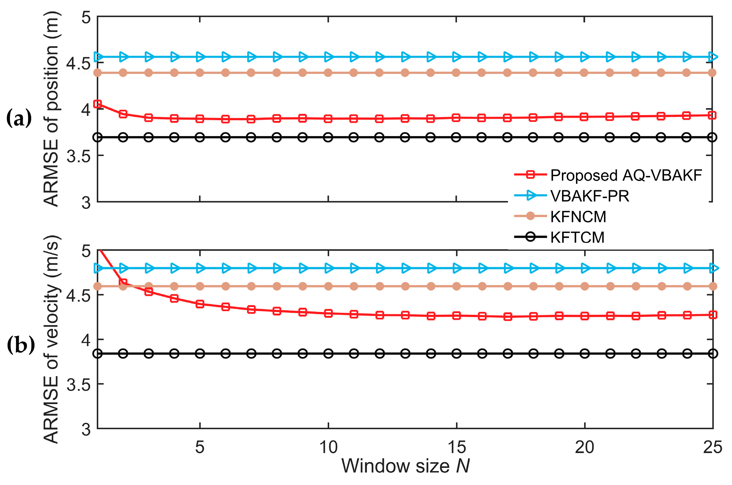
To analyze the effect of the window size on the proposed AQ-VBAKF algorithm, some further simulations are performed. The window size is set as N = 1:1:25, and other parameters are the same as those in Table 1. The ARMSEs of different window sizes are shown in Figure 6. The KFTCM has the smallest ARMSEs of position and velocity, which acts as a reference.

In Figure 6a, the ARMSEs of the position for the proposed AQ-VBAKF are smaller than that for the VBAKF-PR and KFNCM when N = 1:1:25. In Figure 6b, the ARMSEs of the position for the proposed AQ-VBAKF are smaller than that for the VBAKF-PR and KFNCM when N ≥ 4. As we can see, the ARMSEs for both position and velocity cannot decrease as the window size N increases when N = 1:1:25. When the window size N is larger than 10, the ARMSEs for both the position and velocity estimations tend to be stable.

In dynamic conditions, the window size cannot be too large. A small window size can help the innovation covariance adapt to the time-varying input signals [25]. On the other hand, the window size should be large enough to enhance the innovation covariance estimation stability. Moreover, if the window size is too small, the computational burden will be heavier. Accordingly, taking into account the innovation covariance estimation accuracy and computational efficiency simultaneously in the dynamic environment, the window size N should be set as 4 ≤ N ≤ 10.

4.4. Computational Efficiency Comparison

To verify the computational efficiency,

Table 2. Total computational time for different algorithms.

Algorithms	Computational Time (s)
KF	37.7627
AQKF	45.0514
VBAKF	172.4772
VBAKF-PR	356.0744
Proposed AQ-VBAKF	188.0822

shows the total simulation time for the different algorithms. The parameter settings are shown in Table 1, and $M_{\mathrm{c}}$ = 1000. The proposed method adds only 9% computational time compared with the VBAKF method and is only about half of the VBAKF-PR simulation time. Therefore, the proposed method has almost the same computational burden compared with the VBAKF algorithm and the computational complexity is not high.

To further evaluate the computational complexity, the total floating-point operations of each step for the proposed AQ-VBAKF were analyzed and are shown in

Table 3. Floating-point operations of proposed AQ-VBAKF algorithms.

Steps	Floating-Point Operations
1	$2n_x{}^2-n_x$
2	$6n_x{}^2{n}_z+4n_x{n}_z{}^2+2n_z+5n_z{}^2-1$
3	$2n_x{}^3+2n_x{}^2$
4, 5, 6	$S(2n_x{}^2{n}_z+2n_x{n}_z{}^2+n_x{n}_z+n_z+3n_z{}^2+3)$
7	$S(2n_x{}^3+6n_x{}^2{n}_z-n_x{}^2+n_x{n}_z+4n_x{n}_z{}^2+n_z{}^2)$

, where $n_x$ and $n_z$ are the dimensions of the state vector and measurement vector, respectively. $S$ is the VB iteration time.

According to Table 3, the total floating-point operations of the proposed AQ-VBAKF are:

$$\begin{array}{ll}f{l}_{\mathrm{AQ-VBAKF}}& =2n_x{}^3+4n_x{}^2+6n_x{}^2{n}_z-n_x+4n_x{n}_z{}^2+2n_z+5n_z{}^2-1\\ & +S(2n_x{}^3+8n_x{}^2{n}_z-n_x{}^2+6n_x{n}_z{}^2+2n_x{n}_z+4n_z{}^2+n_z+3)\end{array}$$

(47)

Based on [14,17], the total floating-point operations of VBAKF-PR are:

$$\begin{array}{ll}f{l}_{\mathrm{VBAKF-PR}}& =2n_x{}^3+4n_x{}^2+n_z{}^2+1\\ & +S[n_x{}^3+O(2n_x{}^3)+4n_x{}^2{n}_z+3n_x{n}_z{}^2+O(3n_z{}^3)+2n_x{}^2+4n_x{n}_z+2n_z{}^2]\end{array}$$

(48)

Based on Equations (47) and (48), $f{l}_{\mathrm{AQ-VBAKF}}$ and $f{l}_{\mathrm{VBAKF-PR}}$ are almost proportional to the VB iteration times S. Substrating Equation (48) to (47), then:

$$\begin{array}{l}f{l}_{\mathrm{VBAKF-PR}}-f{l}_{\mathrm{AQ-VBAKF}}=-6n_x{}^2{n}_z+n_x-4n_x{n}_z{}^2-2n_z-4n_z{}^2+1\\ +S[-n_x{}^3+O(2n_x{}^3)-4n_x{}^2{n}_z+3n_x{}^2-3n_x{n}_z{}^2+2n_x{n}_z+O(3n_z{}^3)-2n_z{}^2-n_z-3]\end{array}$$

(49)

According to Equation (49), with the increase in the VB iteration time S, the computational burden of VBAKF-PR is larger than the proposed AQ-VBAKF, which is consistent with the computational time results.

5. Conclusions

This paper proposes a novel AQ-VBAKF algorithm that can adjust the PNCM and MNCM simultaneously. This algorithm introduces the adaptive factor to self-tune the PNCM in real time based on the input signals. Furthermore, the MNCM is estimated online using the VB approximation. According to the dynamic target tracking test results, the proposed AQ-VBAKF shows more accurate estimation and better robustness in comparison with other filtering methods. Moreover, for a general case in practical systems, when the initial PNCM and MNCM are not appropriately set and deviate from the true values, the proposed algorithm has better self-adaptability and robustness than other algorithms. The proposed algorithm’s computational burden is not heavy; thus, it can be applied in practical engineering applications.

For future prospects, the proposed filtering estimation algorithm can be applied in dynamic conditions, such as autonomous vehicles, target tracking, positioning, and so on. For example, autonomous vehicles inherently work under dynamic environments, and the environment noise statistics are unknown. The adaptability of the proposed AQ-VBAKF algorithm can adjust process and measurement noise covariances dynamically, which can significantly enhance the vehicle’s perception accuracy and response. Our research provides a theoretical basis in terms of dynamic conditions to enhance the filtering estimation accuracy. In future work, the proposed algorithm will be employed in positioning systems to enhance positioning accuracy.

References

- Yuan, H.; Song, X. A Modified EKF for Vehicle State Estimation with Partial Missing Measurements. IEEE Signal Process. Lett. 2022, 29, 1594–1598. [Google Scholar] [CrossRef]
- Qiang, X.; Xue, R.; Zhu, Y. Two-Dimensional Monte Carlo Filter for a Non-Gaussian Environment. Electronics 2021, 10, 1385. [Google Scholar] [CrossRef]
- Yuan, T.; Zhao, R. LQR-MPC-Based Trajectory-Tracking Controller of Autonomous Vehicle Subject to Coupling Effects and Driving State Uncertainties. Sensors 2022, 22, 5556. [Google Scholar] [CrossRef] [PubMed]
- Cao, J.; Song, C.; Peng, S.; Song, S.; Zhang, X.; Xiao, F. Trajectory Tracking Control Algorithm for Autonomous Vehicle Considering Cornering Characteristics. IEEE Access 2020, 8, 59470–59484. [Google Scholar] [CrossRef]
- López-Salcedo, J.A.; Peral-Rosado, J.A.; Seco-Granados, G. Survey on robust carrier tracking techniques. IEEE Commun. Surv. Tuts. 2014, 16, 670–688. [Google Scholar] [CrossRef]
- Xie, F.; Liang, G.; Chien, Y.-R. Highly Robust Adaptive Sliding Mode Trajectory Tracking Control of Autonomous Vehicles. Sensors 2023, 23, 3454. [Google Scholar] [CrossRef]
- Li, X.; Bar-Shalom, Y. A recursive multiple model approach to noise identification. IEEE Trans. Aerosp. Electron. Syst. 1994, 30, 671–684. [Google Scholar] [CrossRef]
- Jiang, B.; Sheng, W.; Zhang, R.; Han, Y.; Ma, X. Range tracking method based on adaptive “current” statistical model with velocity prediction. Signal Process. 2017, 131, 261–270. [Google Scholar] [CrossRef]
- Zha, F.; Guo, S.; Li, F. An improved nonlinear filter based on adaptive fading factor applied in alignment of SINS. Optik 2019, 184, 165–176. [Google Scholar] [CrossRef]
- Agamennoni, G.; Nieto, J.; Nebot, E.M. Approximate inference in state-space models with heavy-tailed noise. IEEE Trans. Signal Process. 2012, 60, 5024–5037. [Google Scholar] [CrossRef]
- Hou, B.; Wang, J.; He, Z.; Qin, Y.; Zhou, H.; Wang, D.; Li, D. Novel interacting multiple model filter for uncertain target tracking systems based on weighted Kullback–Leibler divergence. J. Frankl. Inst. 2020, 357, 13041–13084. [Google Scholar] [CrossRef]
- Sarkka, S.; Nummenmaa, A. Recursive noise adaptive Kalman filtering by variational Bayesian approximations. IEEE Trans. Automat. Control 2009, 54, 596–600. [Google Scholar] [CrossRef]
- Xu, D.; Wu, Z.; Huang, Y. A new adaptive Kalman filter with inaccurate noise statistics. Circuits Syst. Signal Process. 2019, 38, 4380–4404. [Google Scholar] [CrossRef]
- Huang, Y.; Zhang, Y.; Wu, Z.; Li, N.; Chambers, J. A novel adaptive Kalman filter with inaccurate process and measurement noise covariance matrices. IEEE Trans. Autom. Control 2018, 63, 594–601. [Google Scholar] [CrossRef]
- Ma, J.; Lan, H.; Wang, Z.; Wang, X.; Pan, Q.; Moran, B. Improved adaptive Kalman filter with unknown process noise covariance. In Proceedings of the 21st International Conference on Information Fusion, Cambridge, UK, 10–13 July 2018; pp. 2054–2058. [Google Scholar]
- Xu, H.; Duan, K.; Yuan, H.; Xie, W.; Wang, Y. Black box variational inference to adaptive Kalman filter with unknown process noise covariance matrix. Signal Process. 2020, 169, 107413. [Google Scholar] [CrossRef]
- Huang, Y.; Zhu, F.; Jia, G.; Zhang, Y. A slide window variational adaptive Kalman filter. IEEE Trans. Circuits Syst. II Exp. Briefs 2020, 67, 3552–3556. [Google Scholar] [CrossRef]
- Brown, R.G.; Hwang, P.Y.C. Introduction to Random Signals and Applied Kalman Filtering, 4th ed.; John Wiley & Sons: Hoboken, NJ, USA, 2012; pp. 143–148. [Google Scholar]
- Sarkka, S. Bayesian Filtering and Smoothing; Cambridge University Press: Cambridge, UK, 2013; pp. 56–62. [Google Scholar]
- Tzikas, D.; Likas, A.; Galatsanos, N. The variational approximation for Bayesian inference. IEEE Signal Process. Mag. 2008, 25, 131–146. [Google Scholar] [CrossRef]
- Wang, G.; Wang, X.; Zhang, Y. Variational Bayesian IMM-Filter for JMSs With Unknown Noise Covariances. IEEE Trans. Aerosp. Electron. Syst. 2020, 56, 1652–1661. [Google Scholar] [CrossRef]
- Chen, X.; Cao, L.; Cao, P.; Xiao, B. A higher-order robust correlation Kalman filter for satellite attitude estimation. ISA Trans. 2022, 124, 326–337. [Google Scholar] [CrossRef]
- Fang, J.; Yang, S. Study on innovation adaptive EKF for in-flight alignment of airborne POS. IEEE Trans. Instrum. Meas. 2011, 60, 1378–1388. [Google Scholar]
- Pan, C.; Gao, J.; Li, Z.; Qian, N.; Li, F. Multiple fading factors-based strong tracking variational Bayesian adaptive Kalman filter. Measurement 2021, 176, 109139. [Google Scholar] [CrossRef]
- Gao, W.; Li, J.; Zhou, G.; Li, Q. Adaptive Kalman Filtering with Recursive Noise Estimator for Integrated SINS/DVL Systems. J. Navig. 2015, 68, 142–161. [Google Scholar] [CrossRef]
Figure 1.
Structure diagram of the proposed AQ-VBAKF algorithm.
Figure 2.
RMSEs for different filtering algorithms: (a) the RMSEs of position for different filtering algorithms; (b) the RMSEs of velocity for different filtering algorithms.
Figure 3.
Values of in the proposed AQ-VBAKF algorithm: (a) the mean values of ; (b) the 100th MC test values of ; (c) the 500th MC test values of .
Figure 4.
ARMSEs of position and velocity for the AQ-VBAKF under : (a) ARMSEs of position for the proposed AQ-VBAKF; (b) ARMSEs of velocity for the proposed AQ-VBAKF.
Figure 5.
ARMSEs of position and velocity for the VBAKF-PR algorithm under : (a) ARMSEs of position for the VBAKF-PR; (b) ARMSEs of velocity for the VBAKF-PR.
Figure 6.
ARMSEs of position and velocity under different window sizes N: (a) ARMSEs of position under different window sizes; (b) ARMSEs of velocity under different window sizes.