
Financial Time Series Forecasting: A Data Stream Mining-Based System

1
Computer and System Engineering Laboratory, Faculty of Science and Technology, Cadi Ayyad University, Marrakech 40000, Morocco
2
Innovation Center for the Information Society (CICEI), Campus of Tafira, University of Las Palmas de Gran Canaria, 35017 Las Palmas de Gran Canaria, Spain
*
Author to whom correspondence should be addressed.
†
Current address: Faculty of Sciences and Technology, Cadi Ayyad University, Marrakesh 40000, Morocco.
‡
These authors contributed equally to this work.
Electronics 2023, 12(9), 2039; https://doi.org/10.3390/electronics12092039
Submission received: 19 February 2023
/
Revised: 22 April 2023
/
Accepted: 23 April 2023
/
Published: 28 April 2023
(This article belongs to the Special Issue Advanced Machine Learning Applications in Big Data Analytics)
Abstract
:Data stream mining (DSM) represents a promising process to forecast financial time series exchange rate. Financial historical data generate several types of cyclical patterns that evolve, grow, decrease, and end up dying. Within historical data, we can notice long-term, seasonal, and irregular trends. All these changes make traditional static machine learning models not relevant to those study cases. The statistically unstable evolution of financial market behavior yields a progressive deterioration in any trained static model. Those models do not provide the required characteristics to evolve continuously and sustain good forecasting performance as the data distribution changes. Online learning without DSM mechanisms can also miss sudden or quick changes. In this paper, we propose a possible DSM methodology, trying to cope with that instability by implementing an incremental and adaptive strategy. The proposed algorithm includes the online Stochastic Gradient Descent algorithm (SGD), whose weights are optimized using the Particle Swarm Optimization Metaheuristic (PSO) to identify repetitive chart patterns in the FOREX historical data by forecasting the EUR/USD pair’s future values. The data trend change is detected using a statistical technique that studies if the received time series instances are stationary or not. Therefore, the sliding window size is minimized as changes are detected and maximized as the distribution becomes more stable. Results, though preliminary, show that the model prediction is better using flexible sliding windows that adapt according to the detected distribution changes using stationarity compared to learning using a fixed window size that does not incorporate any techniques for detecting and responding to pattern shifts.
1. Introduction
Financial Time Series Exchange Rate Forecasting (FTSERF) is a growing field because many investors are interested in it. Artificial intelligence, as a computer science sub-field, helped in this development by being part of trading decision systems. Machine learning models became important parts of these systems because they were able to accurately predict the exchange rate and, as a result, increase the chances of making good profits.
When we look at the work done on the algorithms used for FTSERF, we can see that researchers in both public and private institutions have tried out all the machine learning tools that are available. Those tools may be supervised, such as classification [1], regression [2], recommender systems [3], and reinforement learning [4]. They also include unsupervised algorithms, such as clustering and association analysis, ranking, and anomaly detection techniques [5]. The research field of FTSERF using machine learning is wide. Some studies limit their focus to forecasting future trends, while others go beyond that to implement trading strategies that work on maximizing profit.
Speaking about the FTSERF difficulties, dealing with the data’s volatile and chaotic nature is the biggest one. To learn from historical financial time series datasets, you have to be able to adapt to new patterns all the time. This adaptivity is called reacting to the detected changes within the data stream mining (DSM) context. This task is challenging as it requires both recognizing real changes and avoiding false alerts. There are many change detection techniques. Ref. [6] cites some techniques, including the CUSUM test, the geometric moving average test, statistical tests, and drift detection methods.
Our paper’s contribution is to show how integrating DSM techniques into the online learning process can increase FTSERF performance. In our experimental study, we propose the SGD algorithm optimized using the PSO. We managed the changes that occurred in the financial time series trends by implementing a sliding window mechanism. The sliding window size is flexible. It is minimized when a high fluctuation is detected and maximized when the time series pattern is more or less stable. As a change detection mechanism, we test for each sliding window the stationarity of the data stream within, and based on the results, we decide to maintain or adapt the window size that will be passed as input to our forecasting model. We have compared going through the learning process using a traditional algorithm vs. integrating DSM techniques. The traditional algorithm combines the SGD, whose parameters are optimized using the PSO metaheuristic periodically. The DSM version involves the adaptive sliding window mechanism and the statistical stationarity test.
The remainder of this paper is structured as follows. The following section carries out a literature review that we have performed concerning data mining, in addition to DSM’s application to FTSERF. For further illustration, Section 3 is devoted to describing our dataset’s components, its preprocessing, analysis, and input selection processes. Section 4 represents the various proposed forecasting system components and illustrates its architecture and algorithm. Section 4 also shows the various experimental studies, analysis of their results, and further discussions. Finally, some concluding remarks are made in Section 5.
2. Literature Review
2.1. Machine Learning Application to Financial Forecasting
2.1.1. Overview
The financial forecasting research field is very dynamic. The value forecasting of financial assets is a field that attracts the interest of multiple profiles, from accountants, mathematicians, and statisticians to computer scientists. In addition, when it comes to investing, we find that investors with no scientific background easily integrate themselves into the field. Tools like technical analysis are highly used as they are easy to apply and have shown effectiveness in trading. Despite the fact that financial asset markets first appeared in the 16th century (see Figure 1), the first structured approaches to economic forecasting of these assets date from the last century [7,8,9,10].
Research employs methods ranging from mathematical models to statistical models like ARMA, suggested by Wold in 1938 by combining both AR and MA schemes [11], as well as to macroeconomic models like Tinbergen’s (1939) [12]. By this time, various accounting, mathematical, statistical, and machine learning models were constructed to predict different kinds of financial assets, which led to their exponential increase. One of the main apparent reasons for this increase is that this research field is one of the most highly funded, since financial investment generates profit. Funding comes from many sources; we can mainly mention big asset management companies and investment banks.
Back in the 1980s, exploring historical data was more difficult since the amount of data had grown, but computational power was still weak [13]. By the 1990s, more economic and statistical models had appeared, and they showed better performance than a random walk. Still, these models do not perform the same way over all the financial assets [14].
However, by the beginning of the 21st century, machine learning models were all the rage because computers had become faster and were capable of more work. During this time, many hybrid algorithms, such as moving averages that take into account regressivity (ARIMA) or algorithms that combine neural networks and traditional time series, have been proposed. We also noticed the rapid, exponential growth in the number of papers in this research field from 1998 to 2016. There has been a wide range of topics ranging from credit rating to inflation forecasting and risk management, which has saturated this research field and made finding innovative ideas more challenging [13].
On the other hand, scientists became more aware in the 1980s of how important it was to process textual data. There were attempts to import other predictors developed from linguistics by Frazier in 1984 [15]. More progress has been achieved, such as word spotting using naïve statistical methods (Brachman and Khabaza 1996) [16]. Sentiment analysis resources were proposed at the beginning of the 21st century (Hu and Liu 2004) [17]. Sentiment analysis is a critical component that employs both machine learning algorithms and knowledge-based methodologies, particularly for analyzing the sentiments of social media users [18]. From 2010 on, social media data increased exponentially, which attracted the interest of the news analytics community in processing real-time data (Cambria et al. 2014) [13,19].
While reviewing some surveys that shed light on research in financial forecasting, we find some surveys that suggest categorizing the proposed models in different ways. The study in [20] distinguished between singular and hybrid models, which include non-linear models such as artificial neural networks (ANN), support vector machines (SVMs), particle swarm optimization (PSO), as well as linear models like autoregressive integrated moving average (ARIMA), etc. Meanwhile, the study in [21] revealed fundamental and technical analysis as the two approaches that are commonly used to analyze and predict financial market behaviors. It also distinguished between statistical and machine learning approaches, assuming that machine learning approaches deal better with complex, dynamic, and chaotic financial time series. In addition, Ref. [21] points out that the profit analysis of the suggested forecasting techniques in real-world applications is generally neglected. As a solution, they suggest a detailed process for creating a smart trading system. As a solution, it is composed of data preparation, algorithm definition, training, forecasting evaluation, trading strategies, and money evaluation [21]. Papers can also be summarized based on their primary goal, which could be preprocessing, forecasting, or text mining. They can likewise be classified based on the nature of the dataset, whether qualitatively derived from technical analysis or quantitatively retrieved from financial news, business financial reports, or other sources [21]. In addition, Ref. [22] distinguished between parametric statistical methods like Discriminant Analysis and Logistic Regression, Non-Parametric Statistical Methods like Decision Tree and Nearest Neighbor, or Soft Computing techniques like Fuzzy Logic, Support Vector Machine, and Genetic Algorithm.
Essential conclusions are extracted from the survey [21], where it is considered that no approach is better in every way than another, as there is no well-established methodology to guide the construction of a successful, intelligent trading system. Another issue is highlighted in [22] concerning the use of metrics like RMSE and MSE that depend on the scale vs. those that do not, such as the MAPE metric. On the other hand, some papers consider that once a forecasting system is trained, it is expected well in advance to forecast future values. However, this is not possible in the financial time series study case, as they change over time, making retraining with updated data necessary to collect the most recent knowledge about the state of the market. This final issue has been our motivation to work on the DSM application to FTSERF.
2.1.2. Optimization Techniques
In this paper, we combined two optimization techniques, SGD and PSO, as a form of hybridization in order to improve exchange rate forecasting performance.
The gradient descent has been suggested for non-linear problems by Haskell Curry back in 1944 [23]. In the gradient descent, we work on finding the optimal weights for the regression function by minimizing the error loss function. In our study case, the regression function weights depend on the number of explanatory variables used to forecast our target variable. More details about our dataset structure will be shared in a later section. The different types of gradient descent showed great results in dealing with fluctuating patterns, and even with a limited training dataset [24], this makes it an adequate choice for dealing with the chaotic and volatile nature of financial time series. Having an adaptive system is also a must when dealing with change. Gradient descent is flexible enough to be combined with adaptive mechanisms. For example, Ref. [25] propose an adaptive gradient descent willing to deal with a time delay in receiving the input data. SGD can address various types of problems. For example, in [26], a financial continuous-time problem is solved using SGD in continuous time (SGDCT), which showed better results compared to the classic SGD dealing with high-dimensional continuous-time problems. The possibility to combine the SGD with other techniques in order to adapt to the target study’s challenges is a strong point of this algorithm. Another example is the study [27] where a functional gradient descent is proposed in order to forecast the historical interest rate progress possibilities.
The PSO optimization technique is an iterative algorithm that works and converges closer and faster to the solution search space. It is based on a population of solutions collaborating together to reach the optimum results [28]. Despite its limitations, such as the inability to guarantee a good convergence and its computational cost, researchers still use it in financial optimization problems in particular and in other study fields as well, as it helps exceed the convergence limits in many cases. PSO is proposed for the first time by [29,30] as a solution to deal with problems presented in the form of nonlinear continuous functions. In the literature, we find a lot of studies showing how the PSO helped achieve a new score for forecasting time series or any other type of data. In [31], authors have experimented with how PSO can help optimize the results given by neural networks compared to the classic backpropagation algorithm for time series forecasting. On the other hand, the article [32] shows how currency exchange rate forecasting capacity can be polished by adjusting the model function parameters and using the PSO as a booster to the generalized regression neural network algorithm’s performance. Another work combining PSO and neural networks is [33], which worked on predicting the Singapore stock market index. Results demonstrate the effectiveness of using the particle swarm optimization technique to train neural network weights. The performance of the PSO FFNN is assessed by optimizing the PSO settings. In addition, recurrent neural network results predicting stock market behavior have been optimized using PSO in [34]. The study’s findings demonstrate that the model used in this work has a noticeable impact on performance compared to before the hybridization. Finally, we cite [35] where a competitive swarm optimizer that is a PSO variant proved its efficiency dealing with datasets having a large number of features. The experiment shows how the proposed technique can show a fast convergence to greater accuracy.
2.2. Data Stream Mining Application to Financial Forecasting
2.2.1. Data Stream Mining
DSM is the sequence for learning the evolving data stream’s behavior. Data streams could be formed in different data structures, such as trees, particularly ordered and unordered ones. Data streams are present in several study cases, such as financial tickers, network monitoring, traffic management performance metrics, log records, clickstreams for web tracking, etc.
Data stream models need to assume that the sequence of the data that are coming and that are already here is potentially infinite. Thus, it is impossible to keep the data stored. In some circumstances, these models must also handle data in real time since the stream of data might be significant. The distribution of data could change in the future. Thus, historical information could be detrimental to the present situation. The algorithms of data streams have been the subject of extensive research, leading to computer paradigms that optimize memory and time-per-item consumption. The nature of the distribution change has also been studied, where the sliding window approach is used to manage this issue. The oldest element in a window is deleted to receive the newest one. Fixing the window size cannot be prioritized. The change rate needs to be continuously studied since it may itself vary over time [6].
2.2.2. Online Learning
Online learning is one of the main techniques for dealing with data streams. It is a fundamental paradigm of computational learning theory. The algorithms that only employ a small amount of prior data storage are covered under the field of online machine learning in big data streams. After each prediction, an online learner receives the feedback. Online learners are often compared to the top predictors in terms of their excess loss [36,37]. The learning process is called online when it is incremental and adaptive.
For example, effective reinforcement learning is necessary for adaptive real-time machine learning. Due to the nature of online learning, which involves continuous streams of real-time data and adaptive learning from a limited sample size, the algorithm should constantly interact with its environment to optimize the reward [38]. Prequential learning is also one of the efficient techniques used for online learning. It serves as an alternative to the standard holdout evaluation that was carried over from batch-setting issues. The prequential analysis is specifically created for stream environments. Each sample has two distinct functions; it is analyzed sequentially in the order of receipt and then rendered inaccessible. This approach makes predictions for each instance, tests the model, and then trains it using the same sample (partial fit). The model is continually put to the test on fresh samples. Validation techniques are also frequently used to help models be adaptive and incremental. We can mention the following methods: data division into training, test, and holdout groups. We can also cite cross-validation techniques including k-fold, leave-one-out, leave-one-group, and nested. The problem with validation techniques is the risk of overfitting. Techniques for adapting a model are many. We can mention, for example, computing the area under the ROC Curve (AUC) using constant time and memory [39].
2.2.3. Incremental Learning
Incremental learning is a real-time learning approach that builds a similar model as a batch learning algorithm. In theory, the stream of observations could go on indefinitely, making it impossible to wait until all observations are received. Instead of accumulating and storing all inputs and applying batch learning to the full series of received instances, one should apply a batch learning algorithm to each new input [40]. A machine learning paradigm known as incremental learning changes what has already been learned whenever new instances appear. The biggest distinction between incremental learning and classical machine learning is that the former does not presuppose the existence of an appropriate training set before the learning process [41]. Many algorithms, such as neural networks, use epochs to make the model incremental, which helps optimize computational power consumption, especially when dealing with large datasets.
2.2.4. Adaptive Learning
On the other hand, adaptive learning techniques aid in employing a continuously enhanced learning strategy that keeps the system current and maintains its excellent performance. Input and output values, as well as the associated attributes, are continuously monitored and learned through the adaptive learning process. Additionally, it continuously improves its accuracy by learning from events that could change market behavior in real time. Adaptive artificial intelligence takes into account the feedback from the operational environment and responds to it to produce data-driven predictions [42].
Concept drift or changes in the way data are spread out are problems that make it necessary to use adaptive learning techniques. It is a situation where the statistical characteristics of the class variable, or the target we wish to forecast, change with time [43]. Concept drift in machine learning and data mining describes how relationships between the input and output data in the underlying problem vary over time. The concept drift issue is especially prevalent in some areas where forecasts are ordered by time, such as time series forecasting and predictions on streaming data, and it needs to be specifically checked for and addressed [44]. Concept drift can be sudden, gradual, or recurrent. To effectively handle it, a system must be able to quickly adapt, be resilient to noise, be able to separate the noise from it, notice and respond to severe drifts in the model’s performance, and capture up-to-date data trends [45]. For the provided models, techniques, and libraries for data stream classification, we can mention [5], which is a Java-based open-source DSM framework. It also provides regression models. However, more resources are provided when dealing with classification problems.
Machine learning models use different techniques to detect concept drift in classification. We can mention AUC, which detects and adapts to concept drift for classification models. AUC is computed with memory and constant time using a sliding window [46]. AUC evaluates the ranking abilities of a classification. The accuracy metric can be a good choice in the high-class imbalance ratio case, but it may poorly display the concept drift and be biased in identifying the principal class. The foundation for drift identification in unbalanced streams should be AUC. The study in [46] includes Page–Hinkey (PH) statistical test with some updates, include the best outcomes, or very nearly so, except that ADWIN might require more time and memory when change is constant or there is no change.
Regarding concept drift detection for regression problems, there is a technique that consists of studying the eigenvalues and eigenvectors. It allows the characterization of the distribution using an orthogonal basis. This approach is the object of the principal component analysis. A second technique is to monitor covariance. In probability theory and statistics, covariance measures the joint variability of two random variables, or how far two random variables differ when combined. It is also used for two sets of numerical data, calculating deviations from the mean. The covariance between two random variables, X and Y, is 0 if they are independent. The opposite, however, is untrue [47]. For further details, Ref. [48] shows the covariance matrix types. The cointegration study is another technique that detects concept drift, identifying the sensitivity degree of two variables to the same average price over a specified period. The use of it in econometrics is common. It can be used to discover mean-reversion trading techniques in finance [49]. In our study, we compared the use of a fixed versus a flexible window size. We are also involved in studying the stationary process thing the AUC in the process. We conclude that class inequality has an impact on both prequential accuracy and AUC. However, AUC is statistically more discriminant. While accuracy can only reveal genuine drifts, it shows both real and virtual drifts. The authors used post hoc analysis, and the results confirm that AUC performs the best but has issues with highly imbalanced streams. Another family of methods is adaptive decision trees. It can adaptively learn from the data stream, and it is not necessary to understand how frequently or quickly the stream will change [6]. The ADWIN window is also a great technique for adaptive learning. We can either fix its size or make it variable. ADWIN is a parameter-free adaptive size sliding window. When two large sub-windows are too different, the window’s older section is dropped. ADWIN reacts when sudden, infrequent or slow, gradual changes occur. To evaluate ADWIN’s performance, we can follow the accuracy evolution of the false alarm probability, the probability of accurate detection, and the average delay time in detection. Some hybrid models, such as ADWIN with the Kalman filter, have demonstrated that they producat is related to regression problems; more details about it will be explained in the preliminaries section.
2.2.5. Implications of Econometric Methods
For a complete and successful real-world investment strategy in financial market assets, financial economics theory employment is recommended. It is needed to study factors such as time, risks, and investment costs and how they can play a major role in encouraging or discouraging a certain decision. Having agents that are economy-oriented in an investment strategy decision system can prevent the limitations that machine learning would present. Data science and financial economics-oriented agents can work together for more profitable approaches and better forecasting systems. In this context, we cite [50], where authors used machine learning to predict intra-day realized volatility. The study considered stock market crashes such as the European debt crisis, the China–United States trade war, and COVID-19. They tested multiple machine learning algorithms: seasonal autoregressive integrated moving averages (SARIMA), heterogeneous autoregressive with diurnal effects (HAR-D), ordinary least squares (OLS), least absolute shrinkage and selection operator (LASSO), XGBoost, multilayer perceptron (MLP), and long short-term memory (LSTM). They used three training schemes, where in the singular scheme they built distinct models for each stock. The universal scheme consists of constructing models with all stock data. The third training scheme, which is called the augmented scheme, also works on constructing models with all stock data except that predictors take into account market volatility. Training, validation, and testing sets are used in the training process. General results showed the advantage of incorporating volatility, which enhanced the forecasting ability. This study can show how the combination of machine learning and finance knowledge can lead to better predictions and more efficient decision systems.
The paper in [51] has also conducted an interesting study where forecasting simulations are made using econometric methods and other simulations are carried out using machine learning methods. The experiment reveals the importance of considering financial factors such as market maturity in addition to technical factors such as the used forecasting methods and evaluation metrics for good forecasting performance. Results show how Support Vector Machines (SVMs), which is a machine learning method, have given better results than the autoregressive model (AR), which is an econometric method. Advanced machine learning techniques show efficiency in detecting market anomalies in numerous significant financial markets. Authors also criticize studies that judge machine learning efficiency based on experiments applying traditional models instead of advanced ones like sliding windows and optimization mechanisms. They also refer to the fact that forecasting results do not necessarily lead to good returns. In addition to that, many researchers do not consider the transaction cost in their trading simulations.
In the literature, we can find multiple research studies showing how financial and machine learning methods can both contribute to efficient financial forecasting and investment systems. The study in [52] shows how combining statistical and machine learning metrics enhances the forecasting system’s evaluation performance. They compare the forecasting abilities of well-known machine learning techniques: multilayer perceptrons (MLP) and support vector machine (SVM) models, the deep learning algorithm, and long short-term memory (LSTM), in order to predict the opening and closing stock prices for the Istanbul Stock Exchange National 100 Index (ISE-100). The evaluation metrics used are MSE, RMSE, and . In addition, statistical tests are made using IBM SPSS statistics software in order to evaluate the different machine learning models’ results. The findings of this study demonstrate how favorable MLP and LSTM machine learning models are for estimating opening and closing stock prices. Authors of the study in [53] also recommended combining fundamental economic knowledge with machine learning systems, as experts’ judgment strengthens ultimate risk assessment. Their experiment compared machine learning algorithms to a statistical model in risk modeling. The study shows how extreme gradient boosting (XGBoost) succeeds in generating stress-testing scenarios surpassing the classical method. However, the lack of balance complicates class detection for machine learning models. Another challenge is that their dataset was limited to the Portuguese environment and needs to be expanded to other markets in order to improve the system’s validation.
We also find finance and economy-oriented papers that have explored machine learning algorithms and proved their efficiency to forecast financial market patterns and generate good returns for investors. For example, authors in [7] demonstrated how asset pricing with machine learning algorithms is promising in finance. They implemented linear, tree, and neural network-based models. They used machine learning portfolios as metastrategies, where the first metastrategy combines all the models they have built and the second one selects the best-performing models. Results show how high-dimensional machine learning approaches can approximate unknown and potentially complex data-generating processes better than traditional economic models.
We also cite the study in [54], which shows how institutional investors use machine learning to estimate stock returns and analyze systemic financial risks for better investment decisions. The authors concluded that big data analysis can efficiently contribute to detecting outliers or unusual patterns in the market. They also recommend data-driven or data science-based research as a promising avenue for the finance industry.
Despite its efficiency in forecasting, machine learning applications in financial markets have some limitations. For example, authors in [55] concluded that machine learning systems’ performance can vary depending on the studied market conditions. They evaluated the following machine learning algorithms: elastic net (Enet), gradient-boosted regression trees (GBRTs), random forest (RF), variable subsample aggregation (VASA), and neural networks with one to five layers (NN1–NN5). In addition, they tested ordinary least squares (OLS), regression LASSO, an efficient neural network, and gradient-boosted regression trees equipped with a Huber loss function. They encountered difficulties when using data from the US market but achieved good results as they worked on the Chinese stock market time series. However, their experiment did not involve advanced optimization techniques for hyperparameter selection and adaptation to each time series nature.
An interesting book that compares econometric models to machine learning models is [56]. The study shows how econometrics leans more toward statistical significance, while machine learning models focus more on the data’s behavior over time. Machine learning advantages include the fact that they do not skip important information related to data interaction, unlike econometric models. In addition, machine learning models have the capacity to break down complex trends into simple patterns. They also better prevent overfitting using validation datasets. On the other hand, econometric models’ advantage is the fact that their results are explicable, unlike those of machine learning methods, whose learning process includes black boxes. Overall, the references provide valuable insights into the advantages and limitations of machine learning and econometric models in financial forecasting and highlight the need for careful evaluation and interpretation of their results. In our current work, we focused on showing how DSM techniques can boost online algorithms to adapt to financial time series data with time-varying characteristics. Statistical methods play a major role in our system, as we use the stationarity test to detect if there is a change in the data stream distribution.
2.2.6. Data Stream Mining Application to Financial Forecasting
Data mining involves machine learning, statistics, information retrieval, and pattern recognition. The DSM handles data mining tasks as well as the volume, speed, and shifting patterns of data streams. The DSM technique improves and maintains the model’s performance using pattern mining. As older data stream distribution can become irrelevant or damaging to the forecasting accuracy, fitting to newer data using adaptive learning is a must. The DSM is a recent machine learning domain that appeared as a result of multiple domains that generate data streams.
Mining changing data streams employs multiple methods. They must save excellent information, forget useless information, and enhance the model. We can mention as an example the sliding window technique, which retains W data items in a window. New elements replace the oldest ones, where a time t element expires at the time t + W for the sake of memory optimization. The window size W may adjust with the data distribution pace, either externally or during the learning process [6].
The scientists in the FTSERF field using machine learning models have benefited from various incremental and adaptive approaches. They have also proposed novel approaches and hybridized the existing ones. Most of these studies involve adaptive or incremental techniques that are not among the DSM approaches. Few works concretely involved them compared to the total. We can cite [57,58], where sliding windows are used. In those works, adaptivity has been ensured using optimization techniques. For [57], the used technique is called ELM-Jaya, where the final solution is based on the most effective and the weakest solutions. The parameters are adapted in the study in [58] thanks to the PSO metaheuristic, Genetic Algorithm (GA), and neural networks, which are adaptive algorithms by nature.
Incremental approaches include, for example, the uni-iterative approach, where the model receives one instance at each iteration, as in [59,60]. Secondly, multi-iterative systems have multiple instances instead of one. Refs. [61,62] are examples of this type. The third technique is the sliding window. As examples of studies we can cite [63,64]. The sliding window algorithm has a maintained window that keeps instances that have been read most recently, and according to specified rules, older examples are removed [6]. The fourth technique deals with real-time learning, which is efficient but could face difficulties due to the time factor’s strictness. Online learning is the process of making predictions about a series of instances, one after another, and being rewarded or penalized for each one. Before making a prediction, the learner often receives a description of the situation. The learner’s objective is to maximize the cumulative benefit or, conversely, reduce the cumulative loss [65]. Finally, we find no incremental studies in the literature that can be used for batch learning, such as [66,67]. A set or a series of observations are accepted as a single input by a batch learning algorithm. The algorithm creates its model, and it does not continue to learn. In contrast to online learning, batch learning is standing [65].
Adaptive approaches include several categories; we can mention concept drift for change detection to update decision systems, as in [68,69]. Secondly, forgetting factors are highly used in the FTSERF field, and they are especially dedicated for models that rely on weight updates for model tuning. Refs. [70,71] are two examples from this category. The third technique we mention is the order selection technique. It analyzes statistics, makes decisions based on sentimental analysis modules, and votes, such as in [72,73]. The fourth technique is pattern selection, which entails identifying profitable patterns and testing them, as in [74,75]. Last, the weight update is a very common technique. It consists of using new data to adjust the system parameters, or weights. It is proposed in many studies, such as in [76,77]. More information concerning the state of the art of DSM application for FTSERF will be presented in another work, our global survey.
3. Preliminaries
3.1. Dataset Description
In our dataset, we have chosen to include three currency pairs. The EUR/USD pair represents our target to forecast, while the GBP/USD and the JPY/USD pairs are included because of their significant impact and correlation to our target pair. Each pair’s historical data have open, high, low, and close prices. The dataset we used ranges from 30 May 2000 to 28 February 2017, later expanded to 30 November 2022. More information can be found in the data availability statement.
Our dataset also integrated 12 technical indicators calculated for each one of the three used pairs: the stochastic oscillator, the Relative Strength Index (RSI), the StochRSI oscillator, the Moving Average Convergence and Divergence (MACD), the average directive index (ADX), the Williams% R, the Commodity Channel Index (CCI), the true mean range (ATR), the High-Low index, the ultimate oscillator, the Price Rate Of Change Indicator (ROC), the Bull power, and the Bear power. In addition, we used historical gold price data in Euro, US Dollar, British Pound, and Japanese Yen.
3.2. Dataset Preprocessing
Data preprocessing is a significant step between the data collection and the algorithm learning phases. It can use techniques like data transformation, encoding, and feature engineering to make the dataset easy for the algorithm to understand and work with. We may exclude at this phase unnecessary or redundant features. The exclusion can also be because of the weak correlation and impact on the target variable. Speaking about data preprocessing for DSM, the study in [78] provides a detailed survey. The authors cited how they converted unprocessed information into high-quality input. Techniques like integration, normalization, purification, and transformation are involved. In addition, the study integrated data reduction techniques, discretizing complex continuous feature spaces by choosing and removing unnecessary and distracting features.
In our experimental study, we first started with the input data granularity unification on a daily basis. Then we calculated for each one of the three pairs of time series from j-1 (1 day before the current value) to j-6 (6 days before the current value). The next step was calculating the technical indicators using their mathematical formulas. The process has been performed using a Python code we developed to make the process easy to repeat every time a new input comes. Further details will be shared in the dataset analysis and the experimental sections.
3.3. The Dataset Analysis and the Input Selection
The next step that follows the data preprocessing is the data analysis. It allows an understanding of the relevance of the data, and it also facilitates the choice of the algorithm to be used in the learning process. The data analysis includes three main steps: the univariate analysis, the bivariate analysis, and the multivariate analysis.
Whether we are looking at a qualitative or a quantitative feature changes how the univariate analysis is performed. In this analysis, we can study the following characteristics: the first quartile Q1, the minimum, the third quartile Q3, the median, the deciles, the 95th percentile, the 5th percentile, the maximum, the variance, the standard deviation, the range, the variable dispersion, and the symmetry index (skewness).
The bivariate analysis leads to linear links by restriction, transformation, or by studying the linear correlation. We test the strength of the correlation using the Pearson correlation coefficient, the H0 test, multiple linear regression, covariance, the assumptions of the simple linear model, the variance analysis table (ANOVA), the estimators table, and model validation methods like Anscombe.
The multivariate analysis techniques help choose the best combination of features and carry out the data dimension reduction. One of the most commonly used techniques is principal component analysis (PCA) [79].
Tests have been made in our previous work [2]. In Figure 2, we can see that dispersed residuals along a horizontal line without clear patterns are equally distributed on the upper and lower sides of the line. It is also noticeable that residuals have non-linear patterns. As we do not have any non-linear correlations, linear regression is a reasonable option for our study case.
Figure 3 shows that the residuals follow a straight line in the middle and do not deviate in a severe way, indicating that our quantile sets do in fact originate from normal distributions. However, residuals at the extremities curve off. This behavior typically indicates that our historical data have more extreme instances than would be expected if they really came from a normal distribution.
The spread-location plot is depicted in Figure 4. The residuals are distributed equally over the predictor ranges, and the horizontal line with evenly dispersed points supports the assumption of an equal variance.
Figure 5 displays the residual in relation to the leverage. Extreme values that might have an impact on a regression line can be seen in the lower right corner, outside of a dashed line, or at very few of Cook’s distance points. These examples have an impact on the regression results, so excluding them will change the results.
The FactorMiner module in RStudio’s PCA method is used for feature selection. It condensed the 147 columns to 30 variables with 99 percent of the information. The number of columns is depicted in Figure 6 together with the percentage of data that each one can carry. It aids in the optimization of memory usage during learning.
3.4. Methodologies Adopted
3.4.1. The Stationary Process
The stationary process is the technique we used in our proposed architecture. A stochastic process that is stationary in mathematics and statistics is one whose characteristics or probability distribution do not change as time passes. As a result, variables like the mean and the variance also remain constant over time [80]. Mathematically, a family of random variables is the typical definition of a stochastic or random process. Time series can be used to represent a variety of stochastic processes. A time series, on the other hand, is a collection of observations with integer indexes, but a stochastic process is continuous. The stochastic process is a process in which the characteristic variables undergo random fluctuations [81].
3.4.2. Stochastic Gradient Descent
The gradient descent algorithm reduces a function to its smallest value iteratively. The gradient descent algorithm is summarized in the formula below in a single line.
As we draw a random line through some of these data points in the space, this straight line’s equation would be Y = mX + b, where m is the slope and b is the Y-axis intercept. A machine-learning model tries to predict what will happen with a new set of inputs based on what happened with a known set of inputs. The discrepancy between the expected and actual values would be the error:
The concept of a cost function or a loss function is relevant here. The loss function calculates the error for a single training example in order to assess the performance of the machine learning algorithm.
The cost function, on the other hand, is the average of all the loss functions from the training samples. If the dataset has N total points and we want to minimize the error for each of those N points, the total squared error would be the cost function. Any machine learning algorithm’s goal is to lower the cost function. To do this, we identify the value of X that results in the value of Y that is most similar to actual values. To locate the cost function minima, we devise the gradient descent algorithm formula [82].
The gradient descent algorithm looks like this:
Repeat until convergence
The SGD is similar to the gradient descent algorithm structure, with the difference that it processes one training sample at each iteration instead of using the whole dataset. SGD is widely used for training large datasets because it is computationally faster and can be processed in a distributed way. The fundamental idea is that we can arrive at a location that is quite near the actual minimum by focusing our analysis on just one sample at a time and following its slope. SGD has the drawback that, despite being substantially faster than gradient descent, its convergence route is noisier. Since the gradient is only roughly calculated at each step, there are frequent changes in the cost. Even so, it is the best option for online learning and big datasets.
3.4.3. PSO Metaheuristic Optimization Technique
Metaheuristics apply to discrete problems, and they can also adapt to continuous problems. These methods are stochastic, dealing with the combinatorial explosion of possibilities. They are inspired by physics and biology (such as evolutionary algorithms or ethology). They also share the same drawbacks: the difficulties of adjusting the method’s parameters and the lengthy computation [83].
From the point of view of a particle, the PSO idea works by spreading a fleet of randomly made particles around a search space. Each particle has its own random speed and can evaluate its position to determine its best performance. This model is a good tool for solving linear and mixed-number problems and for situations where the numbers are mixed or continuous. More details about the PSO algorithm we used in our experimental study can be found in [2,83].
4. Experimental Setup and Analysis
4.1. The Proposed Architecture
During our survey, we noticed several techniques ensuring that the proposed system is adaptive, incremental, and consequently learning online. We can mention among adaptive approaches penalization for wrong predictions, higher weighting to more recent data, rewarding techniques, forgetting factors to ancient data, retraining, metaheuristics for parameter adapting, learning rate optimization, sliding windows, and iterations until the performance metric is optimized.
During our experimentation, we have chosen to study the paper in [57]. Their architecture shows an online model that processes financial data streams. They employ a sliding window of size 12, the model is incremental, and the system is adaptive by selecting a solution based on their best and worst performances. The model is tested in various cases: containing the dataset’s statistical metrics, containing technical indicators, and both. In the experimental studies, their model predicts the next day, the following 3, 5, 7 and 15 days, and the following month. Additionally, they employ a variety of learning models, including Teaching Learning-Based Optimization (TLBO), the Jaya optimization method, Neural Networks (NNs), Functional Link Artificial Neural Networks (FLANNs) based on the PSO, and the Differential Evolution (DE) algorithm for weights optimization. Among the performance evaluation metrics they utilized were Theil’s U, Annual Rental Value (ARV), Mean Absolute Error (MAE), and the Mean Absolute Percentage Error (MAPE).
Our idea consists of keeping the window size flexible depending on the concept drift instead of using a fixed window size. We minimize the window size when the concept drift occurs and negatively impacts our current model performance. We maximize the window size if the data trend is stable and no concept drift is detected. Our architecture in Figure 7 is composed of four parts. The first part consists of collecting and scraping the data from the sources we use. The second part focuses on the data preprocessing. In this stage, we first unify the granularity of our historical data on a daily basis, then compute 12 technical indicators for each of the three currency pairs. Online learning starts with the concept of drift detection; this part is responsible for maintaining the stability of our model’s performance by continuously adapting it to new trends. We have tested several techniques and mainly chose the study that tests if the data is stochastic. The presence or absence of concept drift leads to the choice of the window size. The next step will be to fit our model. Since the PSO usage requires more calculations than the SGD alone, we only launch the PSO every 60 days. Using the PSO helps prevent falling into the local minima. Last but not least, we visualize our prediction results and performance metrics progress in several plots and tables.
4.2. The Experiment Environment
The model has been developed using the Anaconda distribution of the Python and R programming languages for scientific computing. Specifically, we used Jupyter Notebook 6.4.12 for coding with Python version 3.9.13. Windows is the operating system where the experiment was carried out.
4.3. The Parameters’ Description
This section explains the different parameters used in our algorithm. We initialized the sliding window size with the value 15, which is likely to be minimized when a change in the time series pattern is detected. We chose 15 because, from our preliminary tests, we saw that, in general, patterns vary from 15 days to another. The variable numRows is our index variable that we use to process the data stream. It is continuously updated by the last instance index that we processed in our model training. The variables rangeMin and rangeMax help us display the instances index from the dataset that our model is being trained with. The PSOApplication parameter helps us count how many days have been processed, so that as soon as we reach 60 days, we launch the PSO optimization technique to help the SGD boost its results.
The PSO parameters are mainly c1 and cmax and are used while updating the weights. xmin and xmax are the range where we try to find our solution. It can be challenging to fix it every time we use a new dataset, and limiting it can take a lot of tests until it is properly fixed. However, once fixed for a particular time series, we continue using it for training and forecasting future values. The number of particles depends on our time and computational power limitations. In this study, we fixed it at 20 particles after several tests on different values. The parameters vmin and vmax determine the speed of movement in the search space for each particle.
The gradient descent parameters are the tolerance that we use as a condition to stop the optimization. It represents the margin of error that we tolerate once it is reached. xmin and xmax are also given as parameters to the SGD.
4.4. The Proposed Search Algorithm
The model-learning phase is composed of many parts. When new instances are available, the stationarity test is performed to specify the next window size, and then the SGD model receives the new input to update the model parameters. Every 60 days, we update the model using the PSO optimization metaheuristic. Our proposed search Algorithm 1 steps are:
| Algorithm 1: The SGD algorithm optimized using the PSO metaheuristic with an adaptive sliding window |
 |
The implementation of the SGD and PSO is inspired by our previous work, Ref. [2], where we developed the classic gradient descent optimized using Particle Swarm Optimization. We used almost the same gradient descent algorithm for the SGD, as the difference between them is limited to the used training data. For the gradient descent, all the training data are received as an input to the Algorithm 2, and then a backpropagation is applied to adjust the model weights. The SGD algorithm receives a new part of the training data at each iteration and adjusts its weights to that subset of data using a backpropagation.
Figure 8 shows our proposed method flowchart, which consists of adapting the sliding window size based on the stationarity statistical test. After this, the forecasting model receives the sliding window instances as input for validation and training.
| Algorithm 2: Gradient algorithm descent optimized with Particle Swarm Optimization |
 |
4.5. The Performance Evaluation Metrics
The model quality measurement metrics are many, depending on the algorithm type and also on the study case. In our experiment, we evaluated our model using two techniques. The first one is the Mean Square Error (MSE), which represents the loss function we wish to optimize:
The function f(x) is the gradient descent function for predicting our target variable, which is the EUR/USD exchange rate:
Our goal is to find the optimal weights of the regression function in our iterative process by optimizing our loss function. Weights are optimized in our SGD using the following formula, where the tolerance is fixed to 0.001 in our experimental part and the error is simply the difference between the real and predicted value of the target variable, the EUR/USD exchange rate in our case:
Our second metric is a classification metric, where we study the accuracy of predicting if the exchange rate will rise or fall. It is presented in the form of a percent, and its formula is the following:
The third metric we used is average rectified value ARV, which shows the average variation for a group of data points. The forecasting model performs identically if we calculate the mean over the series with ARV = 1. The model is considered worse than just taking the mean if ARV > 1.
4.6. Analysis of Results
This section will discuss the various steps and the evolution of our experimental study. In the first tests, we studied the variance and the MSE of the SGD algorithm during its learning process. As shown in Figure 7, in the model learning phase, the concept drift detector, the stationarity statistical test in this case, is applied, right after the sliding window size is determined accordingly, and then we work on optimizing the exchange rate forecasting margin error of the multilinear regression function that we optimize in our SGD algorithm.
For optimizing the regression model weights, both SGD and PSO every 60 days are involved in our experimental study. In SGD, weights are optimized using the gradient descent weights update, Formula (5), in the part of Algorithm 1 where we give as input the new window to the SGD. The second way weights are updated is based on the PSO formula in Algorithm 2 where the particle speed is added to the weight value:
As illustrated in Algorithm 2, the speed is then calculated based on the the search space range, the best particle weight found, the best swarm weight found, and the current weight.
Figure 9 and Figure 10 show that the SGD itself is making good progress. After receiving 1000 instances, the mean squared error (MSE) became more stable, and the variance reached its best stability after receiving 3000 instances.
We updated the learning rate by adding or subtracting 20% of its value and multiplying it by 0.99 or 1.01. We remarked that the learning rate has no impact on the model performance improvement in the case of our architecture. The results did not change and stayed similar to those obtained with the default parameters. As we noted, even when making the previously mentioned updates on the learning rate, the error still does not stabilize until the algorithm reaches around 1000 processed instances.
Figure 11 shows the EUR/USD close price historical data from 1 January 2001 to 1 January 2004. We notice that the value range changed completely comparing 2001 and 2002 to 2003 and 2004, revealing the importance of online learning for financial time series processing.
Figure 12 and Figure 13 show the predicted values in orange versus the actual values in blue using the SGD alone. On the other hand, Figure 14 shows the results as we integrate the PSO metaheuristic every 60 days into the learning process. The accuracy for all the plots is good and reaches 82%. This means that the models correctly predict the price direction in 82% of the cases. The added value of the PSO metaheuristic is noticeable in terms of the margin error, which decreases significantly as the price decreases. The PSO helped minimize the margin error between the predicted and actual values as the price crashed between instances 20 and 30.
Figure 15 and Figure 16 show, the EUR/USD daily close price time series and histogram, respectively, from 30/05/2000 to 28/07/2000. The price values show the volatility of the time series data stream that we need to deal with using concept drift detection techniques.
Table 1, Table 2 and Table 3 summarize statistical values such as the mean and the variance. They also contain a p-value that indicates whether the data is stationary or not. If the p-value is higher than 0.05, the null hypothesis (H0) cannot be rejected, and the data are non-stationary. The results show that in the case of this two-month time series, we have a stationary trend every 15 days, but as we study a whole month or two months, the trend is non-stationary.
We made tests to compare the fixed and flexible window sizes. For the fixed-size case, the chosen size is 15 instances at each iteration because, according to our statistical studies, the data tend to have the same pattern every two weeks. For the flexible window size, we study the next 15 days’ stationarity. If the data are stationary, the algorithm receives 15 new instances. If the data are not stationary, the algorithm receives only one new instance.
Table 4 shows the prediction results for year 2000 EUR/USD historical data as it represents the first data received by the system. In most intervals except [75:90], [90:105], and [120:135], the mean squared error for the flexible-size window case exceeds the fixed-size window case. Meanwhile, for all intervals, we notice that the accuracy using the flexible-size window exceeds or equals the accuracy given using a fixed-size window. To illustrate the predicted vs. the real values, Figure 17 and Figure 18 show the interval [60:74]. We can see that at each point, the real and predicted values are closer in the flexible approach compared to the fixed window approach. The ARV results are all way smaller than 1, which means that our model predicts way better than simply taking the mean. ARV also shows the data points’ variation, and from the obtained values, we can see that the instances are not too correlated to one another.
4.7. Discussions
Figure 9 shows the regression score variance. We see that the model should perform the learning through multiple sliding windows and receive a certain number of instances to reach the point where we can rely on the proposed algorithm results for decision making.
The same is true for Figure 10, where the mean squared error convergence reached its limit starting from receiving approximately 1000 instances. One of the biggest challenges of using gradient descent algorithms is building a model that converges as much as possible. In addition, the best convergence is not guaranteed with the first algorithm execution. Since the weights are often primarily initialized randomly, little by little we limit the search space of the optimal weights to a smaller range.
The learning rate speeds up as the gradient moves while descending. If you set it too high, your path will become unstable, and if you set it too low, the convergence will be slow. If you set it to zero, your model is not picking up any new information from the gradients. As we worked on updating the learning rate alpha by decreasing or increasing its value, we did not notice a difference, and we still obtained the best convergence beyond receiving 1000 instances. The fact that reducing the error to some extent only requires receiving a certain amount of data may help to explain those results.
On the other hand, Figure 11 reveals the importance of DSM to erase the old irrelevant models and build a newer one that fits the new data trends. However, keeping the irrelevant models aside for potential future use can be a good idea. As for some study cases, patterns can reappear occasionally or periodically.
Figure 12, Figure 13 and Figure 14 compared integrating the PSO metaheuristic to online learning vs. not using it. The positive impact is noticed as the price crashes. The margin error was significantly reduced when the PSO was used. Even though the computational and time costs of using the PSO are higher, integrating it periodically to enhance the forecasting quality is promising.
The volatility illustrated in Figure 15 and Figure 16 is one of the biggest challenges encountered in the FTSERF. It has to be managed by minimizing the risks that it reveals. In cases of high volatility, using flexible sliding windows becomes a must. By doing this, we can guarantee that the windows are the right size to see emerging trends and make wise choices.
As noticed from Figure 17 and Figure 18, flexible sliding windows ensured the suggested algorithm had an optimal duration, accuracy, and error margin. The PSO periodic integration and the adaptive sliding windows achieved the fastest convergence. The training and forecasting performances of the algorithm with a flexible window size are better when we compare them to those of the learning algorithm with a fixed window size.
In traditional machine learning, the future fluctuations are adjusted based on previous expectation errors. It consists of investing historical knowledge about past fluctuations, and the model is making decisions or forecasts based on the training it went through. However, as we integrate DSM techniques, adaptive expectations are also ensured by calculating the statistical distribution for every new data stream. The model receives at each iteration fifteen instances, which are minimized to one instance at each iteration as soon as a high level of volatility is detected in the fifteen instances of the new sliding window, which makes the model more adaptive compared to real-time approaches without data stream mining techniques that work on detecting the change and reacting to it.
5. Conclusions and Perspectives
Our study aims to explore the DSM techniques’ efficiency in financial time series forecasting. We mainly used the SGD, and for weight optimization, we integrated the PSO metaheuristic periodically every 60 days. Our target variable was the Euro’s value relative to the US dollar. The first technique involved in DSM is adaptive sliding windows. We tested the cases of using a flexible window whose size changes depending on the data volatility versus using a fixed sliding window. The second technique involved in DSM is change detection. It is the stationarity statistical study where we test if the time series has a constant variance. The flexible sliding window proved its ability to forecast the price direction, as it achieved better accuracy compared to using a fixed sliding window. The adaptivity with the changes in the dataset patterns also assured better price and value forecasting with less margin error, especially as the PSO is involved. Future work will focus on testing more online models and concept drift techniques for financial time series and comparing the strengths and weaknesses of each one. Further experimental tests can also be performed by including other periods of crisis and testing other financial time series.
Author Contributions
Conceptualization, Z.B.; methodology, Z.B.; software, Z.B.; validation, Z.B.; formal analysis, Z.B.; investigation, Z.B.; resources, Z.B.; data curation, Z.B.; writing—original draft preparation, Z.B.; writing—review and editing, Z.B.; visualization, Z.B.; supervision, O.B. and J.S.-M.; project administration, O.B. and J.S.-M.; funding acquisition, O.B. and J.S.-M. All authors have read and agreed to the published version of the manuscript.
Funding
This work was supported by a scholarship received from Erasmus+ exchange program and funding from Centro de Innovación para la Sociedad de la Información, University of Las Palmas de Gran Canaria (CICEI-ULPGC).
Data Availability Statement
We published the dataset we used in this research at the following link: https://github.com/zinebbousbaa/eurusdtimeseries accessed on 27 March 2023.
Conflicts of Interest
All authors have no conflict of interest to disclose.
Abbreviations
The following abbreviations are used in this manuscript:
| DSM | Data Stream Mining |
| FTSERF | Financial Time Series Exchange Rate Forecasting |
| PSO | Particle Swarm Optimization Metaheuristic |
| SGD | Stochastic Gradient Descent |
References
- Gerlein, E.A.; McGinnity, M.; Belatreche, A.; Coleman, S. Evaluating machine learning classification for financial trading: An empirical approach. Expert Syst. Appl. 2016, 54, 193–207. [Google Scholar] [CrossRef] [Green Version]
- Bousbaa, Z.; Bencharef, O.; Nabaji, A. Stock Market Speculation System Development Based on Technico Temporal Indicators and Data Mining Tools. In Heuristics for Optimization and Learning; Springer: Berlin/Heidelberg, Germany, 2021; pp. 239–251. [Google Scholar]
- Stitini, O.; Kaloun, S.; Bencharef, O. An Improved Recommender System Solution to Mitigate the Over-Specialization Problem Using Genetic Algorithms. Electronics 2022, 11, 242. [Google Scholar] [CrossRef]
- Jamali, H.; Chihab, Y.; García-Magariño, I.; Bencharef, O. Hybrid Forex prediction model using multiple regression, simulated annealing, reinforcement learning and technical analysis. Int. J. Artif. Intell. ISSN 2023, 2252, 8938. [Google Scholar] [CrossRef]
- Bifet, A.; Holmes, G.; Pfahringer, B.; Kranen, P.; Kremer, H.; Jansen, T.; Seidl, T. Moa: Massive online analysis, a framework for stream classification and clustering. In Proceedings of the First Workshop on Applications of Pattern Analysis, PMLR, Windsor, UK, 1–3 September 2010; pp. 44–50. [Google Scholar]
- Bifet, A. Adaptive Stream Mining: Pattern Learning and Mining from Evolving Data Streams; Ios Press: Amsterdam, The Netherlands, 2010; Volume 207. [Google Scholar]
- Thornbury, W.; Walford, E. Old and New London: A Narrative of Its History, Its People and Its Places; Cassell publisher: London, UK, 1878; Volume 6. [Google Scholar]
- Cummans, J. A Brief History of Bond Investing. 2014. Available online: http://bondfunds.com/ (accessed on 24 February 2018).
- BIS Site Development Project. Triennial central bank survey: Foreign exchange turnover in April 2016. Bank Int. Settl. 2016. Available online: https://www.bis.org/publ/rpfx16.htm (accessed on 24 February 2018).
- Lange, G.M.; Wodon, Q.; Carey, K. The Changing Wealth of Nations 2018: Building a Sustainable Future; Copyright: International Bank for Reconstruction and Development, The World Bank 2018, License type: CC BY, Access Rights Type: Open, Post date: 19 March 2018; World Bank Publications: Washington, DC, USA, 2018; ISBN 978-1-4648-1047-3. [Google Scholar]
- Makridakis, S.; Hibon, M. ARMA models and the Box–Jenkins methodology. J. Forecast. 1997, 16, 147–163. [Google Scholar] [CrossRef]
- Tinbergen, J. Statistical testing of business cycle theories: Part i: A method and its application to investment activity. In Statistical Testing of Business Cycle Theories; Agaton Press: New York, NY, USA, 1939; pp. 34–89. [Google Scholar]
- Xing, F.Z.; Cambria, E.; Welsch, R.E. Natural language based financial forecasting: A survey. Artif. Intell. Rev. 2018, 50, 49–73. [Google Scholar] [CrossRef] [Green Version]
- Cheung, Y.W.; Chinn, M.D.; Pascual, A.G. Empirical exchange rate models of the nineties: Are any fit to survive? J. Int. Money Financ. 2005, 24, 1150–1175. [Google Scholar] [CrossRef] [Green Version]
- Clifton, C., Jr.; Frazier, L.; Connine, C. Lexical expectations in sentence comprehension. J. Verbal Learn. Verbal Behav. 1984, 23, 696–708. [Google Scholar] [CrossRef]
- Brachman, R.J.; Khabaza, T.; Kloesgen, W.; Piatetsky-Shapiro, G.; Simoudis, E. Mining business databases. Commun. ACM 1996, 39, 42–48. [Google Scholar] [CrossRef]
- Hu, M.; Liu, B. Mining and summarizing customer reviews. In Proceedings of the Tenth ACM SIGKDD International Conference on Knowledge Discovery and Data Mining, Seattle, WA, USA, 22–25 August 2004; pp. 168–177. [Google Scholar]
- Ali, T.; Omar, B.; Soulaimane, K. Analyzing tourism reviews using an LDA topic-based sentiment analysis approach. MethodsX 2022, 9, 101894. [Google Scholar] [CrossRef]
- Cambria, E.; White, B. Jumping NLP curves: A review of natural language processing research. IEEE Comput. Intell. Mag. 2014, 9, 48–57. [Google Scholar] [CrossRef]
- Rather, A.M.; Sastry, V.; Agarwal, A. Stock market prediction and Portfolio selection models: A survey. Opsearch 2017, 54, 558–579. [Google Scholar] [CrossRef]
- Cavalcante, R.C.; Brasileiro, R.C.; Souza, V.L.; Nobrega, J.P.; Oliveira, A.L. Computational intelligence and financial markets: A survey and future directions. Expert Syst. Appl. 2016, 55, 194–211. [Google Scholar] [CrossRef]
- Gadre-Patwardhan, S.; Katdare, V.V.; Joshi, M.R. A Review of Artificially Intelligent Applications in the Financial Domain. In Artificial Intelligence in Financial Markets; Springer: Berlin/Heidelberg, Germany, 2016; pp. 3–44. [Google Scholar]
- Curry, H.B. The method of steepest descent for non-linear minimization problems. Q. Appl. Math. 1944, 2, 258–261. [Google Scholar] [CrossRef] [Green Version]
- Shao, H.; Li, W.; Cai, B.; Wan, J.; Xiao, Y.; Yan, S. Dual-Threshold Attention-Guided Gan and Limited Infrared Thermal Images for Rotating Machinery Fault Diagnosis Under Speed Fluctuation. IEEE Trans. Ind. Inform. 2023, 1–10. [Google Scholar] [CrossRef]
- Lv, L.; Zhang, J. Adaptive Gradient Descent Algorithm for Networked Control Systems Using Redundant Rule. IEEE Access 2021, 9, 41669–41675. [Google Scholar] [CrossRef]
- Sirignano, J.; Spiliopoulos, K. Stochastic gradient descent in continuous time. Siam J. Financ. Math. 2017, 8, 933–961. [Google Scholar] [CrossRef] [Green Version]
- Audrino, F.; Trojani, F. Accurate short-term yield curve forecasting using functional gradient descent. J. Financ. Econ. 2007, 5, 591–623. [Google Scholar]
- Bonyadi, M.R.; Michalewicz, Z. Particle swarm optimization for single objective continuous space problems: A review. Evol. Comput. 2017, 25, 1–54. [Google Scholar] [CrossRef]
- Kennedy, J.; Eberhart, R. Particle swarm optimization. In Proceedings of the ICNN’95-International Conference on Neural Networks, Perth, WA, Australia, 27 November–1 December 1995; IEEE: Piscataway, NJ, USA, 1995; Volume 4, pp. 1942–1948. [Google Scholar]
- Shi, Y.; Eberhart, R. A modified particle swarm optimizer. In Proceedings of the 1998 IEEE International Conference on Evolutionary Computation Proceedings. IEEE World Congress on Computational Intelligence (Cat. No. 98TH8360), Anchorage, AK, USA, 4–9 May 1998; IEEE: Piscataway, NJ, USA, 1998; pp. 69–73. [Google Scholar]
- Jha, G.K.; Thulasiraman, P.; Thulasiram, R.K. PSO based neural network for time series forecasting. In Proceedings of the 2009 International Joint Conference on Neural Networks, Atlanta, GA, USA, 14–19 June 2009; IEEE: Piscataway, NJ, USA, 2009; pp. 1422–1427. [Google Scholar]
- Wang, K.; Chang, M.; Wang, W.; Wang, G.; Pan, W. Predictions models of Taiwan dollar to US dollar and RMB exchange rate based on modified PSO and GRNN. Clust. Comput. 2019, 22, 10993–11004. [Google Scholar] [CrossRef]
- Junyou, B. Stock Price forecasting using PSO-trained neural networks. In Proceedings of the 2007 IEEE Congress on Evolutionary Computation, Singapore, 25–28 September 2007; IEEE: Piscataway, NJ, USA, 2007; pp. 2879–2885. [Google Scholar]
- Yang, F.; Chen, J.; Liu, Y. Improved and optimized recurrent neural network based on PSO and its application in stock price prediction. Soft Comput. 2021, 27, 3461–3476. [Google Scholar] [CrossRef]
- Huang, C.; Zhou, X.; Ran, X.; Liu, Y.; Deng, W.; Deng, W. Co-evolutionary competitive swarm optimizer with three-phase for large-scale complex optimization problem. Inf. Sci. 2023, 619, 2–18. [Google Scholar] [CrossRef]
- Auer, P. Online Learning. In Encyclopedia of Machine Learning and Data Mining; Sammut, C., Webb, G.I., Eds.; Springer: Boston, MA, USA, 2016; pp. 1–9. [Google Scholar]
- Benczúr, A.A.; Kocsis, L.; Pálovics, R. Online machine learning algorithms over data streams. J. Encycl. Big Data Technol. 2018, 1207–1218. [Google Scholar]
- Julie, A.; McCann, C.Z. Adaptive Machine Learning for Changing Environments. 2018. Available online: https://www.turing.ac.uk/research/research-projects/adaptive-machine-learning-changing-environments (accessed on 1 September 2018).
- Grootendorst, M. Validating your Machine Learning Model. 2019. Available online: https://towardsdatascience.com/validating-your-machine-learning-model-25b4c8643fb7 (accessed on 26 September 2018).
- Gepperth, A.; Hammer, B. Incremental learning algorithms and applications. In European Symposium on Artificial Neural Networks (ESANN); HAL: Bruges, Belgium, 2016. [Google Scholar]
- Li, S.Z. Encyclopedia of Biometrics: I-Z; Springer Science & Business Media: Berlin/Heidelberg, Germany, 2009; Volume 2. [Google Scholar]
- Vishal Nigam, M.J. Advantages of Adaptive AI Over Traditional Machine Learning Models. 2019. Available online: https://insidebigdata.com/2019/12/15/advantages-of-adaptive-ai-over-traditional-machine-learning-models/ (accessed on 15 December 2018).
- Santos, J.D.D. Understanding and Handling Data and Concept Drift. 2020. Available online: https://www.explorium.ai/blog/understanding-and-handling-data-and-concept-drift/ (accessed on 24 February 2018).
- Brownlee, J. A Gentle Introduction to Concept Drift in Machine Learning. 2020. Available online: https://machinelearningmastery.com/gentle-introduction-concept-drift-machine-learning/ (accessed on 10 December 2018).
- Das, S. Best Practices for Dealing With Concept Drift. 2021. Available online: https://neptune.ai/blog/concept-drift-best-practices (accessed on 8 November 2018).
- Brzezinski, D.; Stefanowski, J. Prequential AUC for classifier evaluation and drift detection in evolving data streams. In Proceedings of the International Workshop on New Frontiers in Mining Complex Patterns; Springer: Berlin/Heidelberg, Germany, 2014; pp. 87–101. [Google Scholar]
- Dodge, Y. The Concise Encyclopedia of Statistics; Springer Science & Business Media: Berlin/Heidelberg, Germany, 2008. [Google Scholar]
- Chan, J.; Choy, S. Analysis of covariance structures in time series. J. Data Sci. 2008, 6, 573–589. [Google Scholar] [CrossRef]
- Ruppert, D.; Matteson, D.S. Statistics and Data Analysis for Financial Engineering; Springer: Berlin/Heidelberg, Germany, 2011; Volume 13. [Google Scholar]
- Zhang, C.; Zhang, Y.; Cucuringu, M.; Qian, Z. Volatility forecasting with machine learning and intraday commonality. arXiv 2022, arXiv:2202.08962. [Google Scholar] [CrossRef]
- Hsu, M.W.; Lessmann, S.; Sung, M.C.; Ma, T.; Johnson, J.E. Bridging the divide in financial market forecasting: Machine learners vs. financial economists. Expert Syst. Appl. 2016, 61, 215–234. [Google Scholar] [CrossRef] [Green Version]
- Demirel, U.; Handan, Ç.; Ramazan, Ü. Predicting stock prices using machine learning methods and deep learning algorithms: The sample of the Istanbul Stock Exchange. Gazi Univ. J. Sci. 2021, 34, 63–82. [Google Scholar] [CrossRef]
- Guerra, P.; Castelli, M.; Côrte-Real, N. Machine learning for liquidity risk modelling: A supervisory perspective. Econ. Anal. Policy 2022, 74, 175–187. [Google Scholar] [CrossRef]
- Kou, G.; Chao, X.; Peng, Y.; Alsaadi, F.E.; Herrera-Viedma, E. Machine learning methods for systemic risk analysis in financial sectors. Technol. Econ. Dev. Econ. 2019, 25, 716–742. [Google Scholar] [CrossRef]
- Leippold, M.; Wang, Q.; Zhou, W. Machine learning in the Chinese stock market. J. Financ. Econ. 2022, 145, 64–82. [Google Scholar] [CrossRef]
- Shivarova, A.; Matthew, F. Dixon, Igor Halperin, and Paul Bilokon: Machine learning in Finance from Theory to Practice. 2021. Available online: https://rdcu.be/daRTw (accessed on 8 November 2018).
- Das, S.R.; Mishra, D.; Rout, M. A hybridized ELM-Jaya forecasting model for currency exchange prediction. J. King Saud-Univ.-Comput. Inf. Sci. 2020, 32, 345–366. [Google Scholar] [CrossRef]
- Nayak, S.C. Development and performance evaluation of adaptive hybrid higher order neural networks for exchange rate prediction. Int. J. Intell. Syst. Appl. 2017, 9, 71. [Google Scholar] [CrossRef] [Green Version]
- Yu, L.; Wang, S.; Lai, K.K. An Online BP Learning Algorithm with Adaptive Forgetting Factors for Foreign Exchange Rates Forecasting. In Foreign-Exchange-Rate Forecasting with Artificial Neural Networks; Springer: Boston, MA, USA, 2007; pp. 87–100. [Google Scholar] [CrossRef]
- Soares, S.G.; Araújo, R. An on-line weighted ensemble of regressor models to handle concept drifts. Eng. Appl. Artif. Intell. 2015, 37, 392–406. [Google Scholar] [CrossRef]
- Carmona, J.; Gavalda, R. Online techniques for dealing with concept drift in process mining. In Proceedings of the International Symposium on Intelligent Data Analysis; Springer: Berlin/Heidelberg, Germany, 2012; pp. 90–102. [Google Scholar]
- Yan, H.; Ouyang, H. Financial time series prediction based on deep learning. Wirel. Pers. Commun. 2018, 102, 683–700. [Google Scholar] [CrossRef]
- Barddal, J.P.; Gomes, H.M.; Enembreck, F. Advances on concept drift detection in regression tasks using social networks theory. Int. J. Nat. Comput. Res. (IJNCR) 2015, 5, 26–41. [Google Scholar] [CrossRef] [Green Version]
- Chen, J.F.; Chen, W.L.; Huang, C.P.; Huang, S.H.; Chen, A.P. Financial time-series data analysis using deep convolutional neural networks. In Proceedings of the 2016 7th International Conference on Cloud Computing and Big Data (CCBD), Macau, China, 16–18 November 2016; IEEE: Piscataway, NJ, USA, 2016; pp. 87–92. [Google Scholar]
- Sammut, C.; Webb, G.I. Encyclopedia of Machine Learning; Springer Science & Business Media: Berlin/Heidelberg, Germany, 2011. [Google Scholar]
- Kumar Chandar, S. Fusion model of wavelet transform and adaptive neuro fuzzy inference system for stock market prediction. J. Ambient. Intell. Humaniz. Comput. 2019, 1–9. [Google Scholar] [CrossRef]
- Pradeepkumar, D.; Ravi, V. Forex rate prediction: A hybrid approach using chaos theory and multivariate adaptive regression splines. In Proceedings of the 5th International Conference on Frontiers in Intelligent Computing: Theory and Applications; Springer: Berlin/Heidelberg, Germany, 2017; pp. 219–227. [Google Scholar]
- Wang, L.Y.; Park, C.; Yeon, K.; Choi, H. Tracking concept drift using a constrained penalized regression combiner. Comput. Stat. Data Anal. 2017, 108, 52–69. [Google Scholar] [CrossRef] [Green Version]
- Baier, L.; Hofmann, M.; Kühl, N.; Mohr, M.; Satzger, G. Handling Concept Drifts in Regression Problems–the Error Intersection Approach. arXiv 2020, arXiv:2004.00438. [Google Scholar]
- Maneesilp, K.; Kruatrachue, B.; Sooraksa, P. Adaptive parameter forecasting for forex automatic trading system using fuzzy time series. In Proceedings of the 2011 International Conference on Machine Learning and Cybernetics, Guilin, China, 10–13 July 2011; IEEE: Piscataway, NJ, USA, 2011; Volume 1, pp. 189–194. [Google Scholar]
- Yu, L.; Wang, S.; Lai, K.K. An online learning algorithm with adaptive forgetting factors for feedforward neural networks in financial time series forecasting. Nonlinear Dyn. Syst. Theory 2007, 7, 51–66. [Google Scholar]
- Ilieva, G. Fuzzy Supervised Multi-Period Time Series Forecasting; Sciendo: Warszawa, Poland, 2019. [Google Scholar]
- Bahrepour, M.; Akbarzadeh-T, M.R.; Yaghoobi, M.; Naghibi-S, M.B. An adaptive ordered fuzzy time series with application to FOREX. Expert Syst. Appl. 2011, 38, 475–485. [Google Scholar] [CrossRef]
- Martín, C.; Quintana, D.; Isasi, P. Grammatical Evolution-based ensembles for algorithmic trading. Appl. Soft Comput. 2019, 84, 105713. [Google Scholar] [CrossRef]
- Hoan, M.V.; Mai, L.C.; Hui, D.T. Pattern discovery in the financial time series based on local trend. In Proceedings of the International Conference on Advances in Information and Communication Technology; Springer: Berlin/Heidelberg, Germany, 2016; pp. 442–451. [Google Scholar]
- Yu, L.; Wang, S.; Lai, K.K. Forecasting Foreign Exchange Rates Using an Adaptive Back-Propagation Algorithm with Optimal Learning Rates and Momentum Factors. In Foreign-Exchange-Rate Forecasting with Artificial Neural Networks; Springer: Boston, MA, USA, 2007; pp. 65–85. [Google Scholar]
- Castillo, G.; Gama, J. An adaptive prequential learning framework for Bayesian network classifiers. In Proceedings of the European Conference on Principles of Data Mining and Knowledge Discovery; Springer: Berlin/Heidelberg, Germany, 2006; pp. 67–78. [Google Scholar]
- Ramírez-Gallego, S.; Krawczyk, B.; García, S.; Woźniak, M.; Herrera, F. A survey on data preprocessing for data stream mining: Current status and future directions. Neurocomputing 2017, 239, 39–57. [Google Scholar] [CrossRef]
- Husson, F.; Lê, S.; Pagès, J. Analyse de Données avec R; Presses universitaires de Rennes: Rennes, France, 2016. [Google Scholar]
- Brockwell, P.J.; Davis, R.A. Introduction to Time Series and Forecasting; Springer: Berlin/Heidelberg, Germany, 2002. [Google Scholar]
- Binder, M.D.; Hirokawa, N.; Windhorst, U. Encyclopedia of Neuroscience; Springer: Berlin/Heidelberg, Germany, 2009; Volume 3166. [Google Scholar]
- Pandey, P. Understanding the Mathematics behind Gradient Descent. 2019. Available online: https://towardsdatascience.com/understanding-the-mathematics-behind-gradient-descent-dde5dc9be06e (accessed on 18 March 2019).
- Clerc, M.; Siarry, P. Une nouvelle métaheuristique pour l’optimisation difficile: La méthode des essaims particulaires. J3eA 2004, 3, 007. [Google Scholar] [CrossRef]
Figure 1.
The chronology of financial asset appearance and the existing forecasting approaches for their valuation [7,8,9,10].

Figure 2.
The residuals measure versus the fitted values.

Figure 3.
The normal Q-Q plot.

Figure 4.
The location scale.

Figure 5.
The leverage versus the residuals.

Figure 6.
The data distribution analysis.

Figure 7.
Our proposed architecture.

Figure 8.
The proposed method flowchart.

Figure 9.
The variance regression score progress.

Figure 10.
The MSE regression score progress.

Figure 11.
The EUR/USD close price historical data from 1 January 2001 to 1 January 2004.

Figure 12.
The real vs. the predicted values using the SGD algorithm.

Figure 13.
The real vs. the predicted values using the SGD algorithm on a bigger test dataset.

Figure 14.
The real vs. the predicted values using the SGD algorithm optimized using the PSO metaheuristic every 60 days.
Figure 14.
The real vs. the predicted values using the SGD algorithm optimized using the PSO metaheuristic every 60 days.

Figure 15.
The EUR/USD daily close price time series from 30 May 2000 to 28 July 2000.

Figure 16.
The EUR/USD daily close price histogram from 30 May 2000 to 28 July 2000.

Figure 17.
The flexible window: the predicted vs. the real value for the interval [60:74].

Figure 18.
The fixed window: the predicted vs. the real value for the interval [60:74].


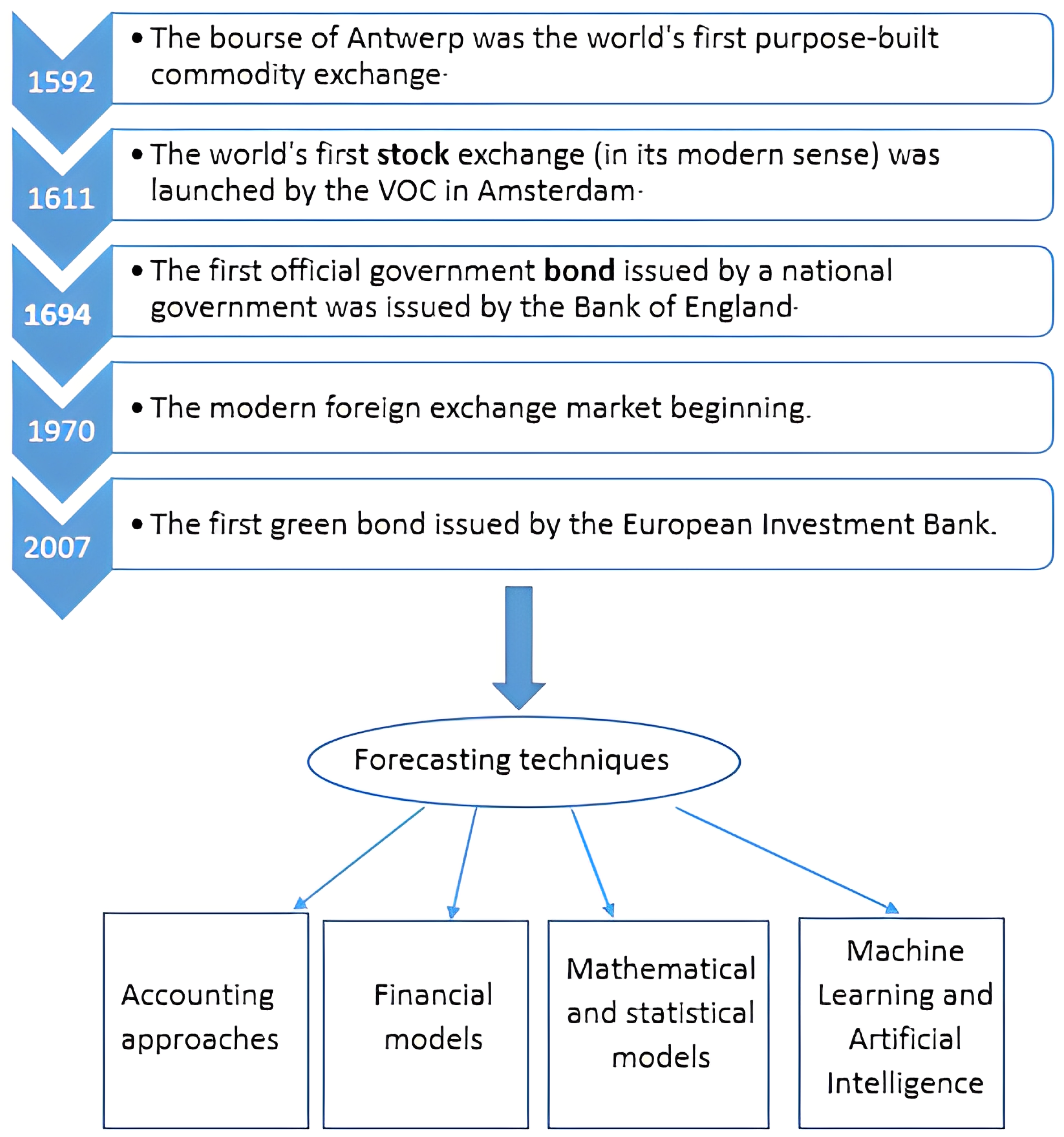
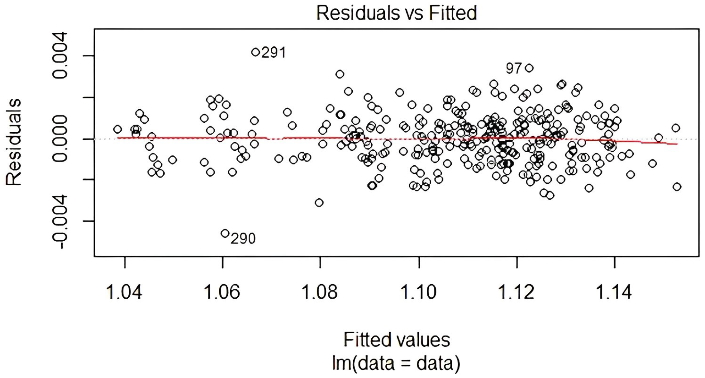
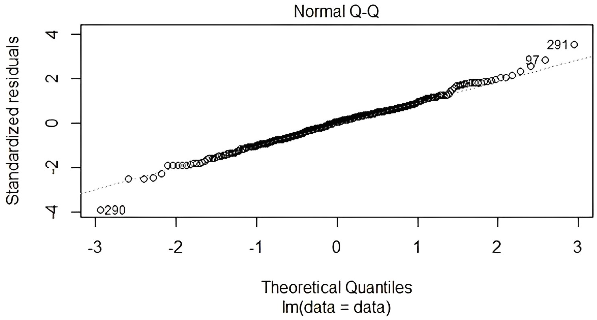
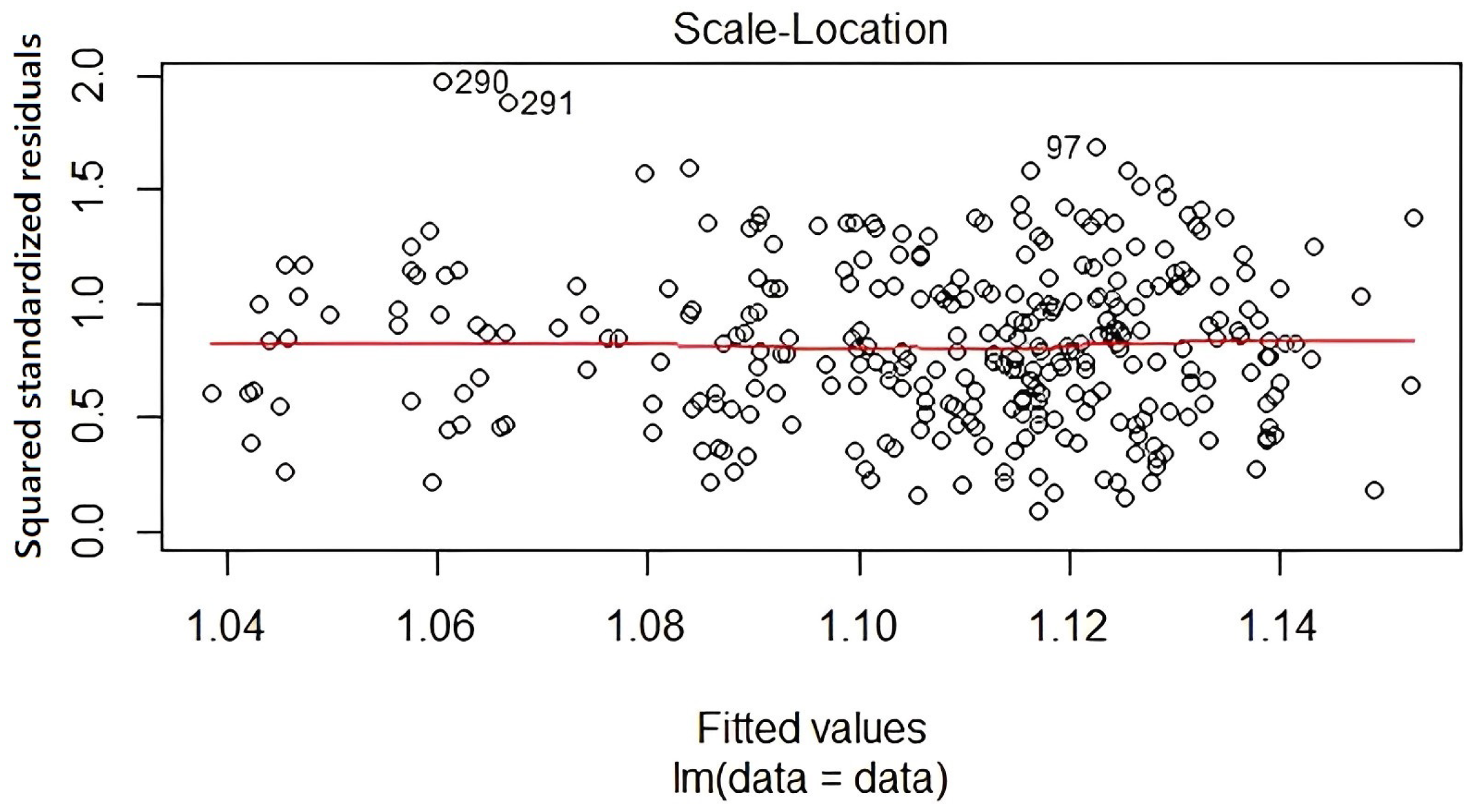
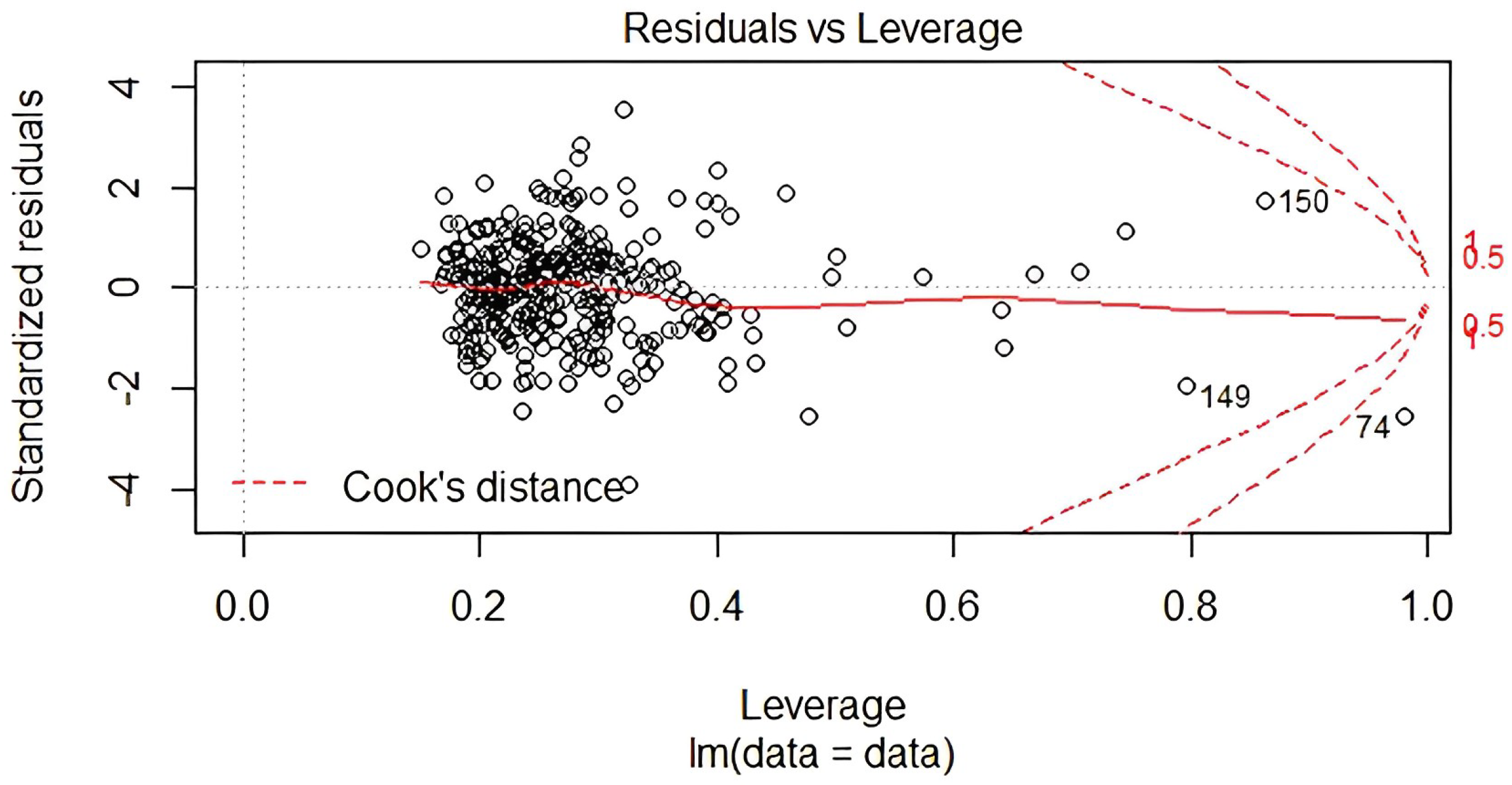
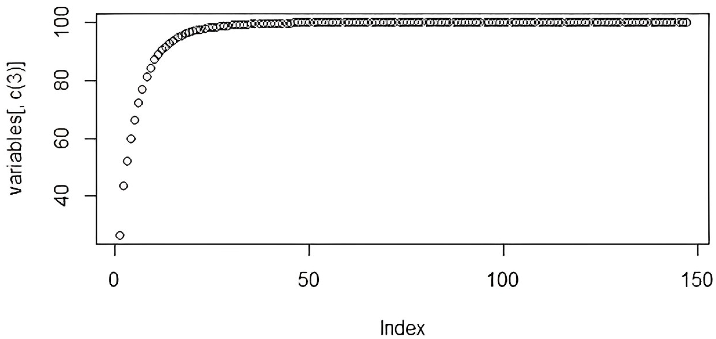
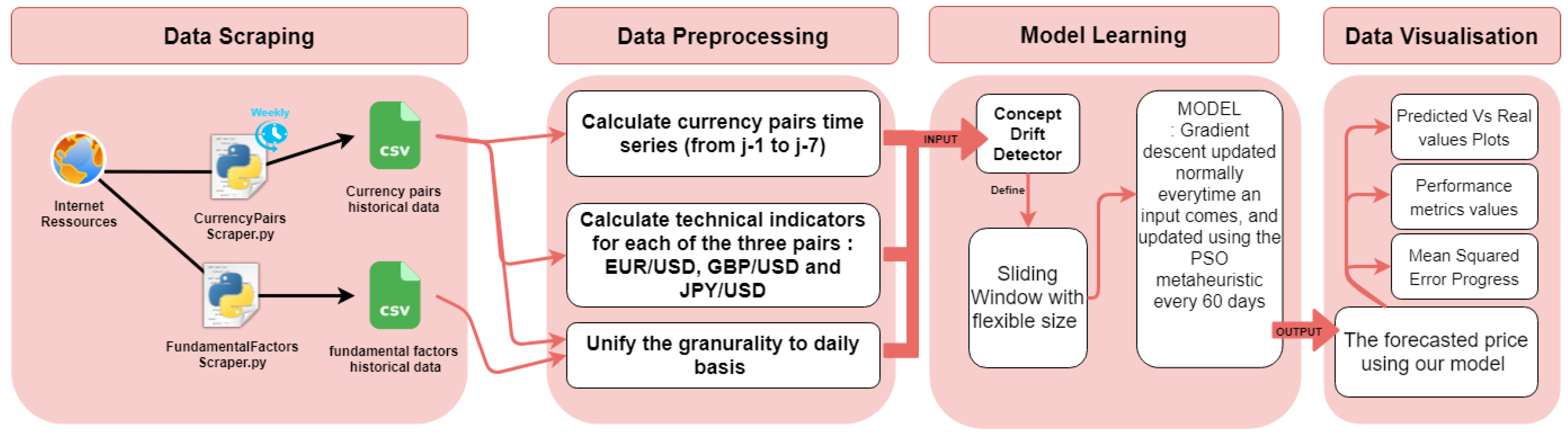
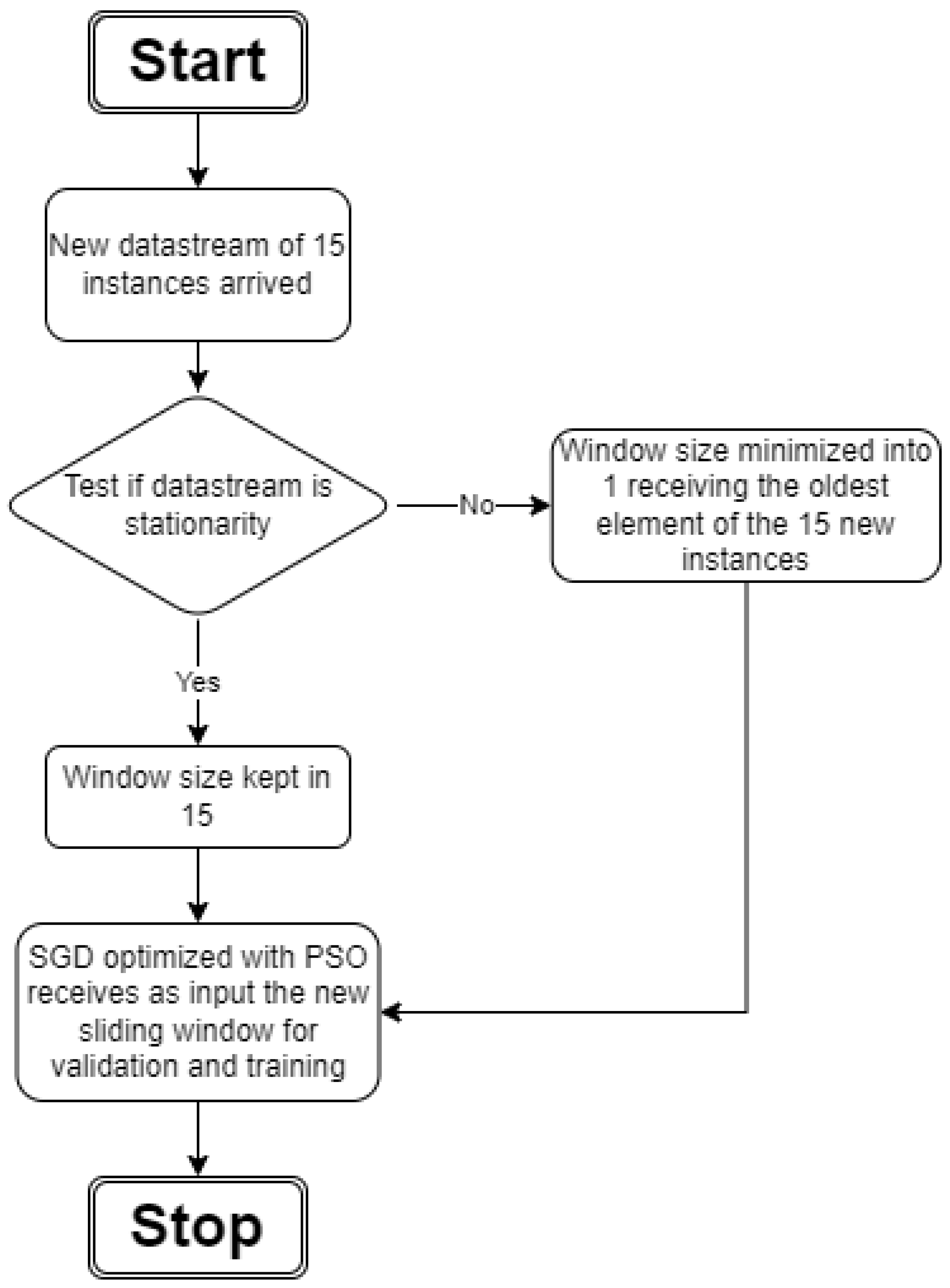
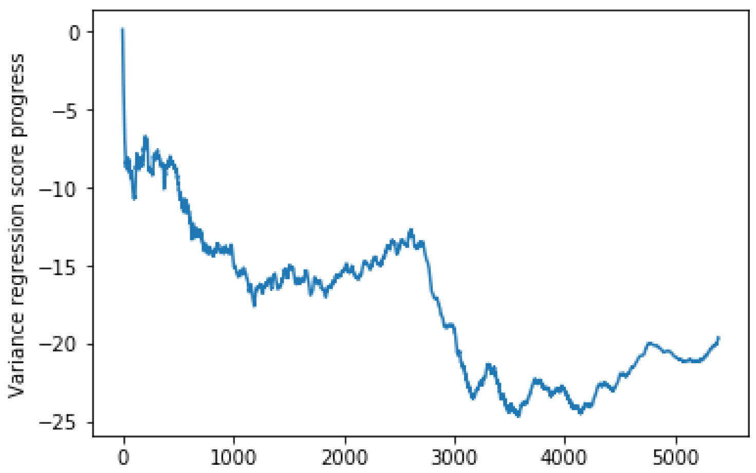
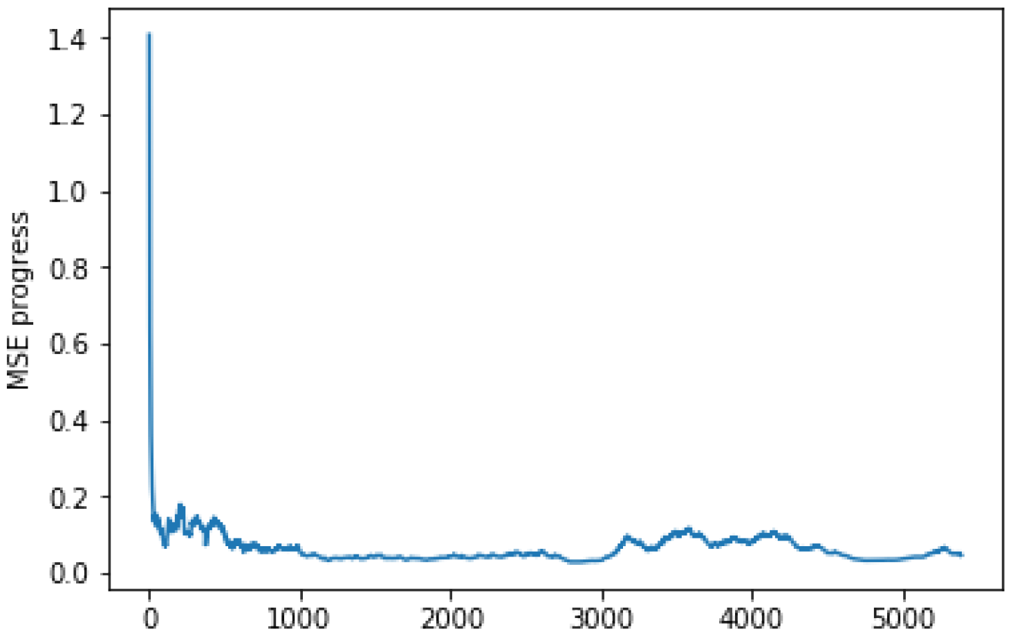
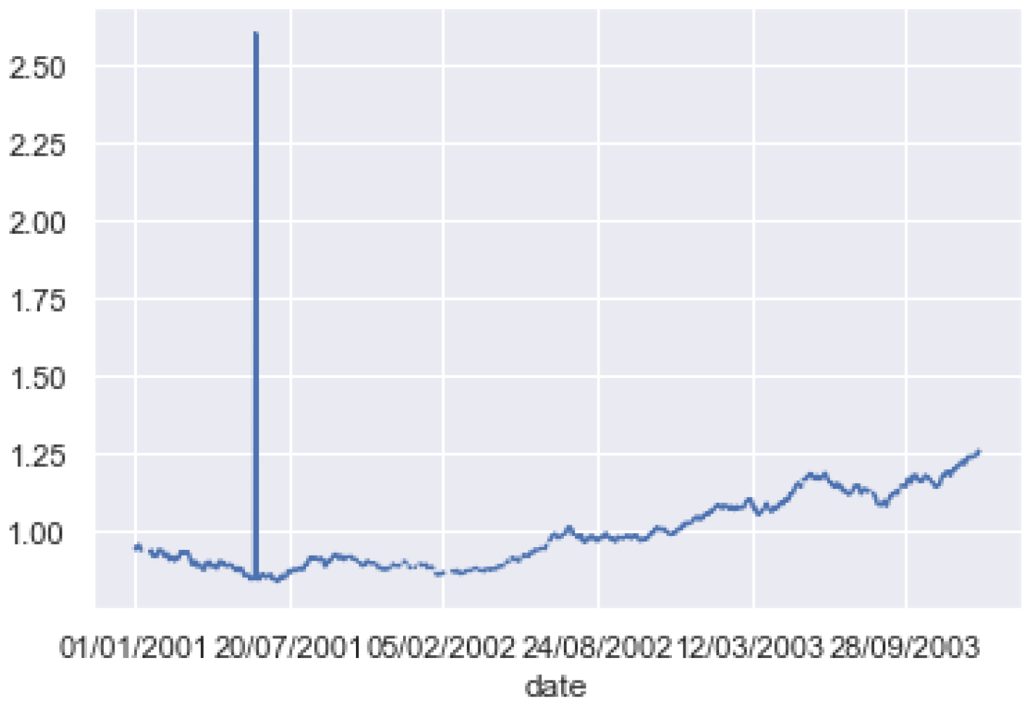
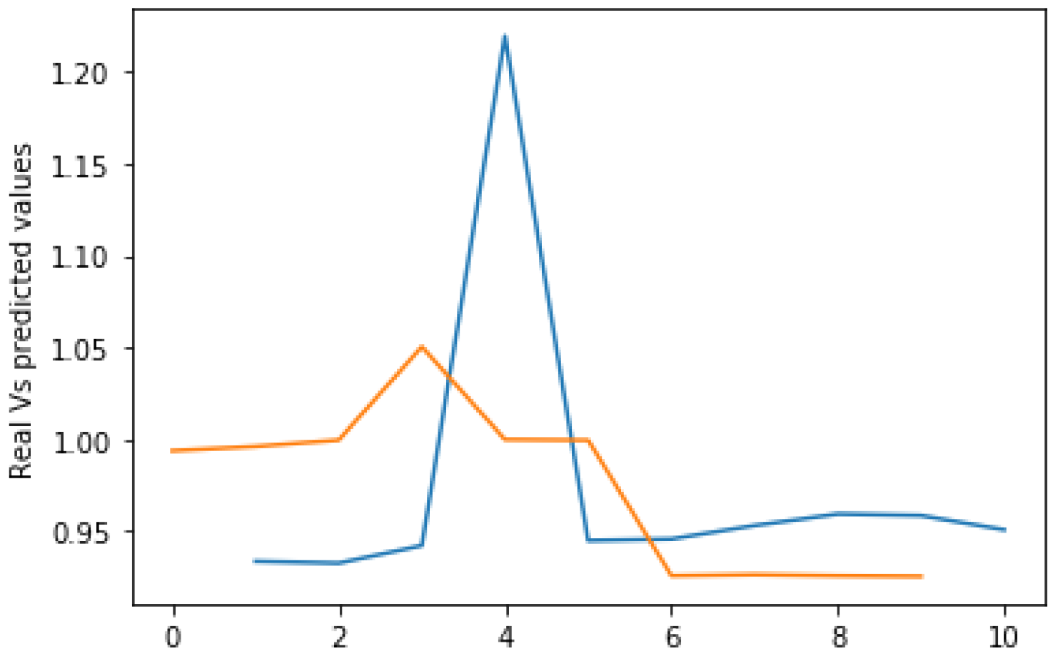
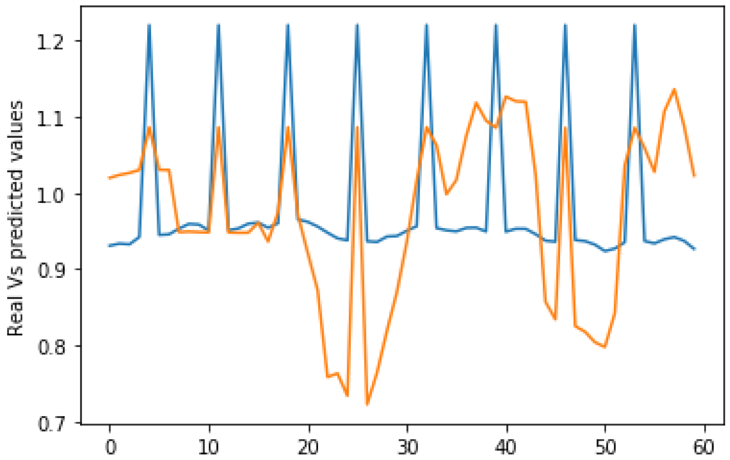
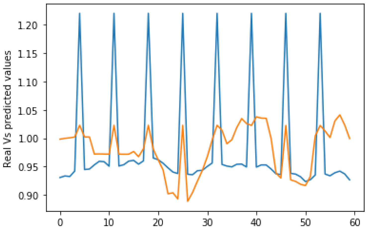
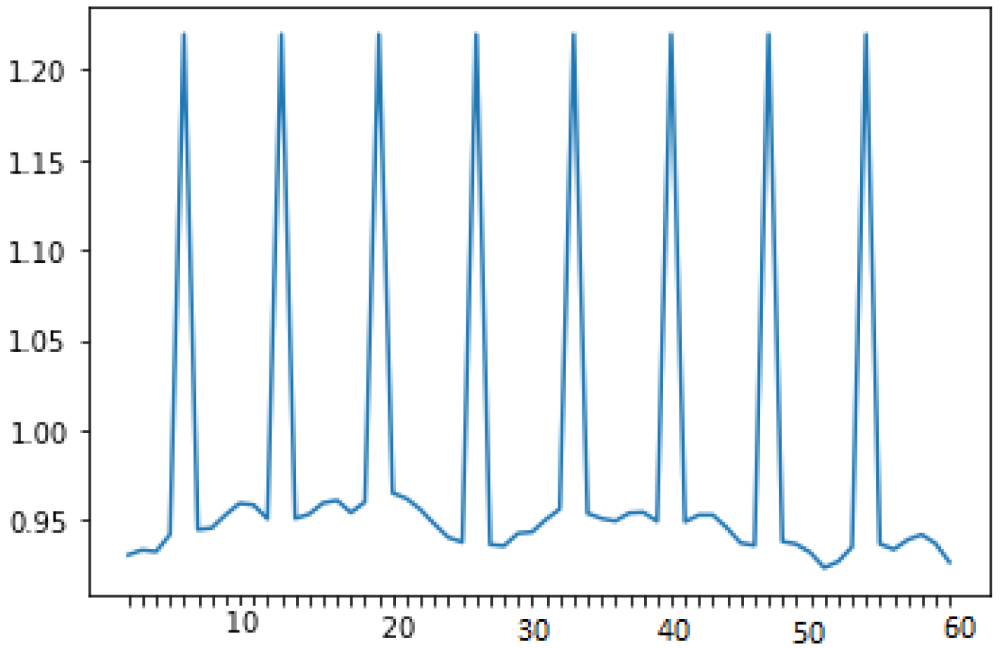
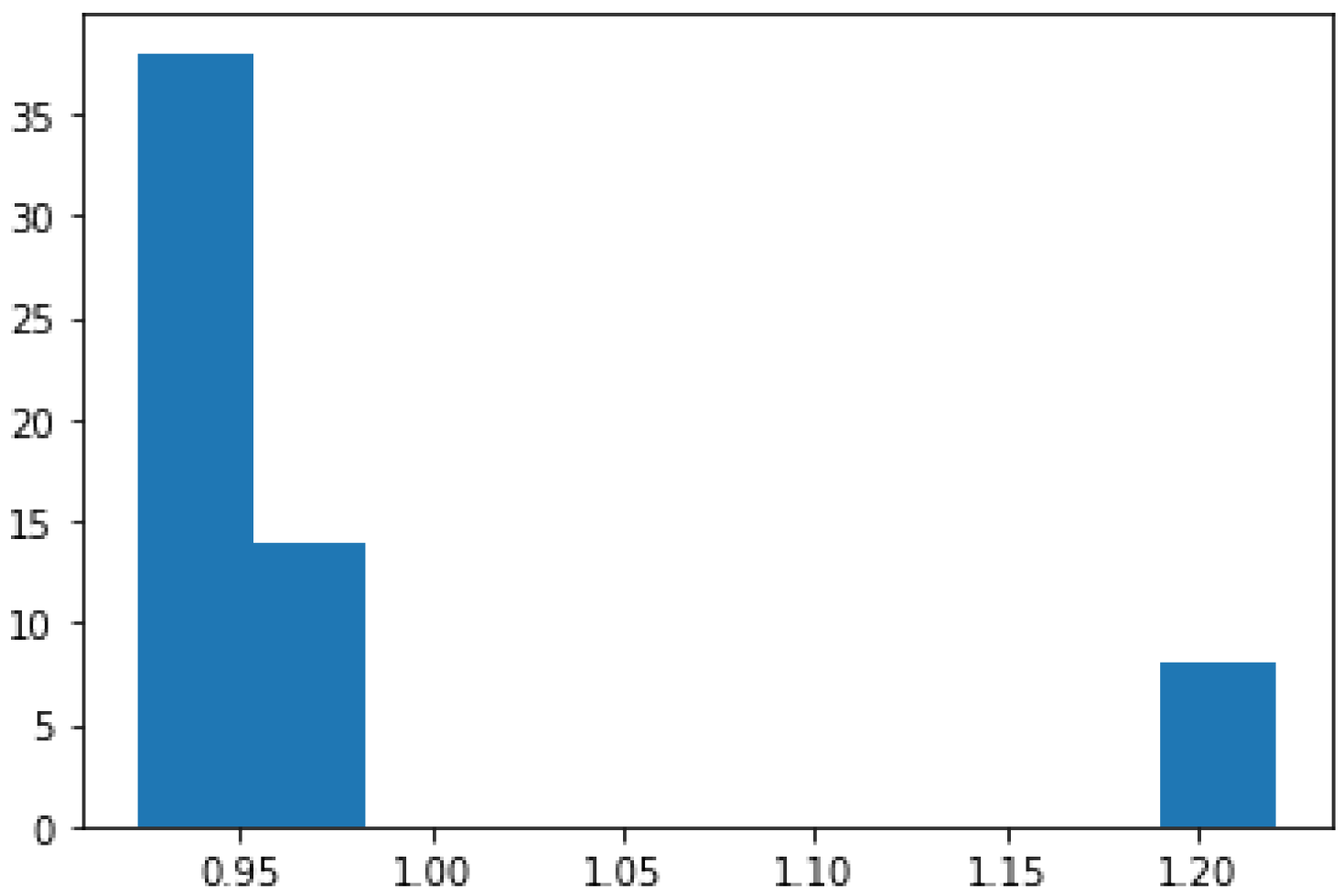
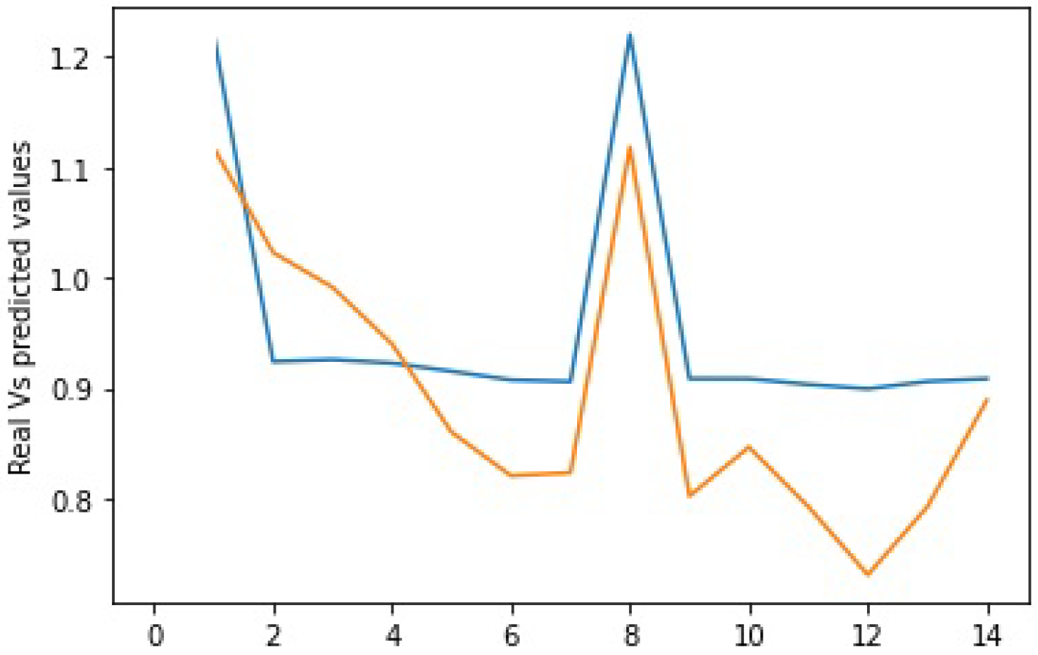
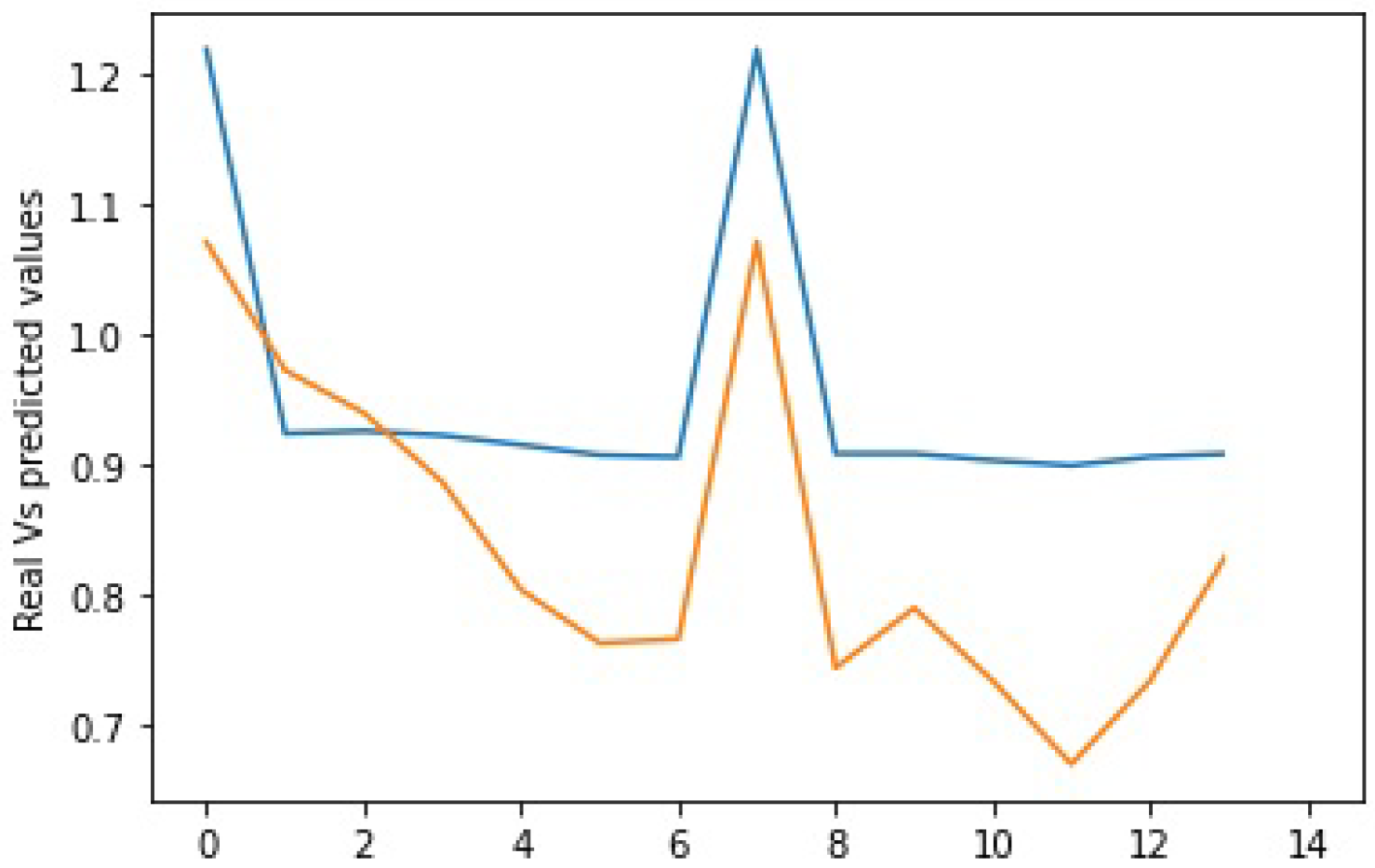
Table 1.
The EUR/USD statistics from 30 May 2000 to 28 July 2000.
| Mean | 0.9819729708789546 |
| Variance | 0.008933902258522159 |
| ADF Statistic | −1.535025 |
| p-value | 0.516119 |
| Critical Values | 1%: −3.563; 5%: −2.919; 10%: −2.597 |
Table 2.
The EUR/USD statistics from 30 May 2000 to 28 July 2000 split into two equal parts.
| Data | 1st 30 Days | 2nd 30 Days |
| Mean | 0.984582 | 0.979364 |
| Variance | 0.008592 | 0.008965 |
| ADF Statistic | −1.084344 | −1.193593 |
| p-value | 0.721275 | 0.676346 |
| Critical Values | 1%: −3.770; 5%: −3.005; 10%: −2.643 | 1%: −3.809; 5%: −3.022; 10%: −2.651 |
Table 3.
The EUR/USD statistics from 30 May 2000 to 28 July 2000 split into four equal parts.
| Data | 1st 15days | 2nd 15days | 3rd 15days | 4th 15days |
| Mean | 0.983657 | 0.985506 | 0.986441 | 0.972288 |
| Variance | 0.008653 | 0.008529 | 0.008389 | 0.009440 |
| ADF Statistic | −4.419853 | −3.628841 | −17.540606 | −16.313688 |
| p-value | 0.000274 | 0.005233 | 0.0 | 0.0 |
| Critical Values | 1%: −4.473 5%: −3.290 10%: −2.772 | 1%: −4.473 5%: −3.290 10%: −2.772 | 1%: −4.473 5%: −3.290 10%: −2.772 | 1%: −4.473 5%: −3.290 10%: −2.772 |
Table 4.
The flexible vs. the fixed sliding window results from year 2000 EUR/USD historical data.
| Flexible Window Size | Fixed Window Size | ||||||
|---|---|---|---|---|---|---|---|
| Range | MSE | ARV | Accuracy | Range | MSE | ARV | Accuracy |
| [0:15] | 0.0027 | 0.0519 | 66.6 | [0:15] | 0.002902 | 0.0538 | 66.6 |
| [1:16] | 0.002534 | 0.0503 | 66.6 | [15:30] | 0.00528 | 0.0726 | 80.0 |
| [2:17] | 0.00237 | 0.0486 | 73.3 | ||||
| [3:18] | 0.00217 | 0.0465 | 73.3 | ||||
| [4:19] | 0.0028 | 0.0529 | 73.3 | ||||
| [5:20] | 0.002 | 0.0447 | 73.3 | ||||
| [6:21] | 0.00192 | 0.0438 | 80.0 | ||||
| [7:22] | 0.00201 | 0.0448 | 86.6 | ||||
| [8:23] | 0.0031 | 0.0556 | 86.6 | ||||
| [9:24] | 0.00404 | 0.0635 | 80.0 | ||||
| [10:25] | 0.00528 | 0.0726 | 80.0 | ||||
| [11:26] | 0.00608 | 0.0779 | 80.0 | ||||
| [26:41] | 0.00727 | 0.0852 | 66.6 | [30:45] | 0.01416 | 0.1189 | 66.6 |
| [27:42] | 0.00658 | 0.0811 | 66.6 | ||||
| [28:43] | 0.00586 | 0.0765 | 66.6 | ||||
| [29:44] | 0.00495 | 0.0703 | 66.6 | ||||
| [30:45] | 0.00494 | 0.0702 | 66.6 | ||||
| [31:46] | 0.00546 | 0.0738 | 66.6 | [45:60] | 0.00607 | 0.0779 | 93.3 |
| [32:47] | 0.00686 | 0.0828 | 66.6 | ||||
| [33:48] | 0.00623 | 0.0789 | 66.6 | ||||
| [34:49] | 0.00699 | 0.0836 | 66.6 | ||||
| [35:50] | 0.00788 | 0.0887 | 73.3 | ||||
| [36:51] | 0.00874 | 0.0934 | 73.3 | ||||
| [37:52] | 0.00917 | 0.0957 | 73.3 | ||||
| [38:53] | 0.00895 | 0.0946 | 73.3 | ||||
| [39:54] | 0.01016 | 0.1007 | 80.0 | ||||
| [40:55] | 0.00887 | 0.0941 | 86.6 | ||||
| [41:56] | 0.00856 | 0.0925 | 93.3 | ||||
| [42:57] | 0.00857 | 0.0925 | 93.3 | ||||
| [43:58] | 0.00874 | 0.0934 | 93.3 | ||||
| [44:59] | 0.00895 | 0.0946 | 93.3 | ||||
| [45:60] | 0.00849 | 0.0921 | 93.3 | ||||
| [46:61] | 0.00922 | 0.096 | 93.3 | [60:75] | 0.00936 | 0.0967 | 73.3 |
| [47:62] | 0.00782 | 0.0884 | 93.3 | ||||
| [48:63] | 0.0071 | 0.0842 | 86.6 | ||||
| [49:64] | 0.00649 | 0.0805 | 86.6 | ||||
| [50:65] | 0.00635 | 0.0796 | 86.6 | ||||
| [51:66] | 0.00657 | 0.081 | 86.6 | ||||
| [52:67] | 0.00709 | 0.0842 | 80.0 | ||||
| [53:68] | 0.00843 | 0.0918 | 80.0 | ||||
| [54:69] | 0.00836 | 0.0914 | 80.0 | ||||
| [55:70] | 0.00908 | 0.0952 | 73.3 | ||||
| [56:71] | 0.01043 | 0.1021 | 73.3 | ||||
| [57:72] | 0.01237 | 0.1112 | 73.3 | ||||
| [58:73] | 0.00573 | 0.0756 | 73.3 | ||||
| [59:74] | 0.00464 | 0.0681 | 73.3 | ||||
| [74:89] | 0.00688 | 0.0829 | 80.0 | [75:90] | 0.0047 | 0.0685 | 80.0 |
| [75:90] | 0.00781 | 0.0883 | 80.0 | ||||
| [76:91] | 0.00917 | 0.0957 | 80.0 | [90:105] | 0.00672 | 0.0819 | 60.0 |
| [77:92] | 0.01095 | 0.1046 | 80.0 | ||||
| [78:93] | 0.0127 | 0.1126 | 86.6 | ||||
| [79:94] | 0.01469 | 0.1212 | 80.0 | ||||
| [80:95] | 0.01651 | 0.1284 | 73.3 | ||||
| [81:96] | 0.01672 | 0.1293 | 73.3 | ||||
| [82:97] | 0.01695 | 0.1301 | 73.3 | ||||
| [83:98] | 0.01727 | 0.1314 | 66.6 | ||||
| [84:99] | 0.01819 | 0.1348 | 66.6 | ||||
| [85:100] | 0.01864 | 0.4317 | 66.6 | ||||
| [86:101] | 0.0186 | 0.1363 | 66.6 | ||||
| [87:102] | 0.01881 | 0.1371 | 66.6 | ||||
| [88:103] | 0.01814 | 0.1346 | 66.6 | ||||
| [89:104] | 0.01837 | 0.1355 | 66.6 | ||||
| [90:105] | 0.01754 | 0.1324 | 60.0 | ||||
| [91:106] | 0.01636 | 0.1279 | 60.0 | [105:120] | 0.03948 | 0.1986 | 53.3 |
| [92:107] | 0.01427 | 0.1194 | 60.0 | ||||
| [93:108] | 0.01176 | 0.1084 | 66.6 | ||||
| [94:109] | 0.00956 | 0.0977 | 73.3 | ||||
| [95:110] | 0.00766 | 0.0875 | 73.3 | ||||
| [96:111] | 0.0074 | 0.086 | 73.3 | ||||
| [97:112] | 0.00712 | 0.0843 | 73.3 | ||||
| [98:113] | 0.00684 | 0.0827 | 66.6 | ||||
| [99:114] | 0.00586 | 0.0765 | 60.0 | ||||
| [100:115] | 0.00486 | 0.0697 | 60.0 | ||||
| [101:116] | 0.00624 | 0.0789 | 66.6 | ||||
| [102:117] | 0.00562 | 0.0749 | 60.0 | ||||
| [103:118] | 0.00836 | 0.0914 | 53.3 | ||||
| [104:119] | 0.01005 | 0.1002 | 60.0 | ||||
| [105:120] | 0.01068 | 0.1033 | 53.3 | ||||
| [120:135] | 0.01108 | 0.10526 | 60.0 | [120:135] | 0.00885 | 0.094 | 60.0 |
Disclaimer/Publisher’s Note: The statements, opinions and data contained in all publications are solely those of the individual author(s) and contributor(s) and not of MDPI and/or the editor(s). MDPI and/or the editor(s) disclaim responsibility for any injury to people or property resulting from any ideas, methods, instructions or products referred to in the content. |
© 2023 by the authors. Licensee MDPI, Basel, Switzerland. This article is an open access article distributed under the terms and conditions of the Creative Commons Attribution (CC BY) license (https://creativecommons.org/licenses/by/4.0/).
Share and Cite
MDPI and ACS Style
Bousbaa, Z.; Sanchez-Medina, J.; Bencharef, O. Financial Time Series Forecasting: A Data Stream Mining-Based System. Electronics 2023, 12, 2039. https://doi.org/10.3390/electronics12092039
AMA Style
Bousbaa Z, Sanchez-Medina J, Bencharef O. Financial Time Series Forecasting: A Data Stream Mining-Based System. Electronics. 2023; 12(9):2039. https://doi.org/10.3390/electronics12092039
Chicago/Turabian StyleBousbaa, Zineb, Javier Sanchez-Medina, and Omar Bencharef. 2023. "Financial Time Series Forecasting: A Data Stream Mining-Based System" Electronics 12, no. 9: 2039. https://doi.org/10.3390/electronics12092039
Note that from the first issue of 2016, this journal uses article numbers instead of page numbers. See further details here.