
Interactive Effect of Learning Rate and Batch Size to Implement Transfer Learning for Brain Tumor Classification
 , and
, and
Abstract
:1. Introduction
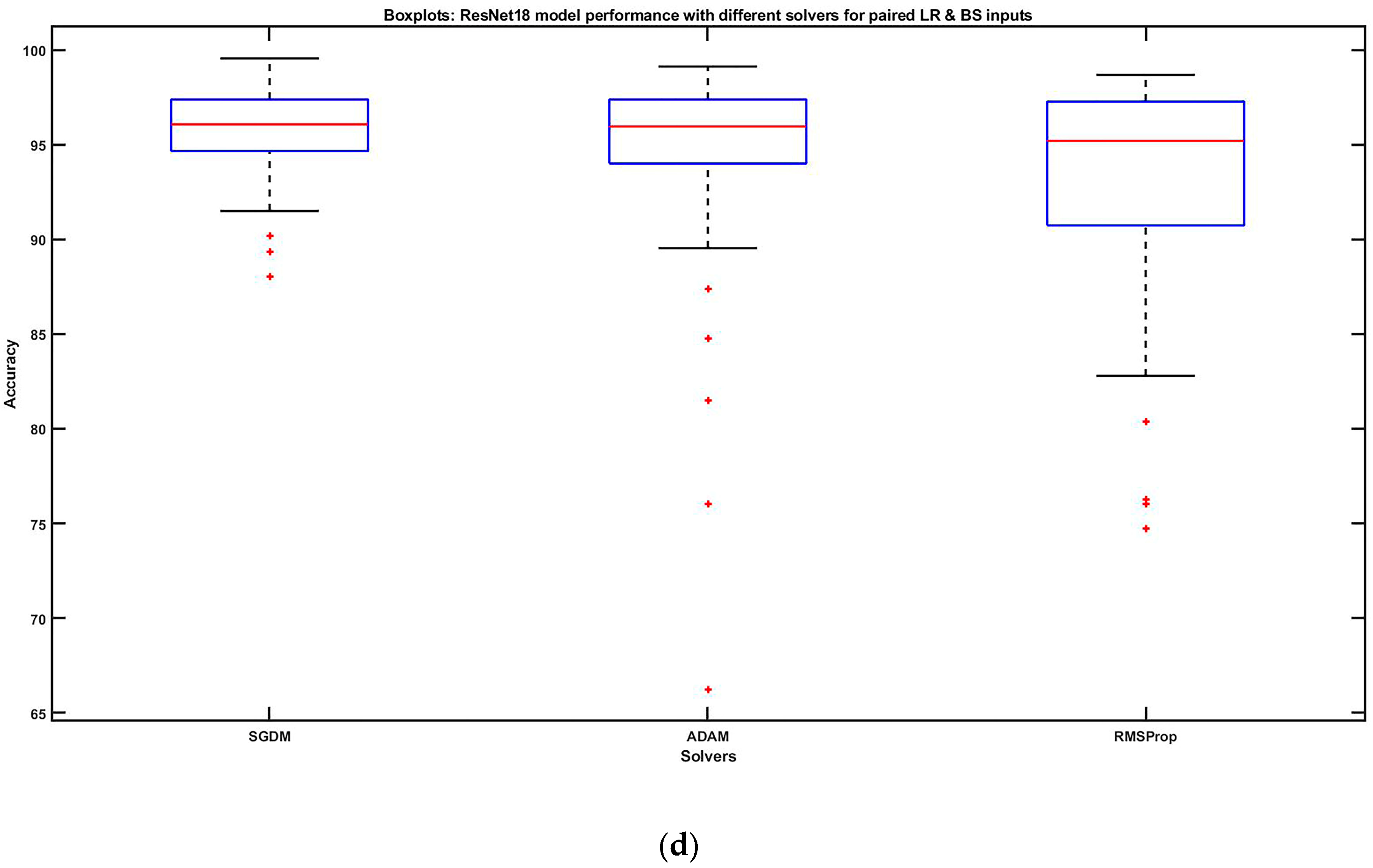
- In comparison to the previous research, for better interpretation, an extended version of a (8 × 7) Cartesian product matrix is generated to evaluate and validate the impact of hyperparameters (LR and BS). The matrix consists of the 56 most effective two-tuple hyperparameters used as an input to perform an extensive exercise, comprising 504 simulations for three cutting-edge architecture-based pre-trained Deep Learning (DL) models, ResNet18, ResNet50, and ResNet101. Additionally, the impact was also assessed by using three well-known optimizers (solvers): SGDM, Adam, and RMSProp.
- A dataset comprising 504 DL model accuracies against each pair of hyperparameters (LR, BS). The accuracies represent model performances trained for brain tumor multi-classification.
- Validation of the simulated results regarding the significant impact of hyperparameters individually as well as interactively using statistical ANOVA analysis.
2. Literature Review
3. Materials and Methods
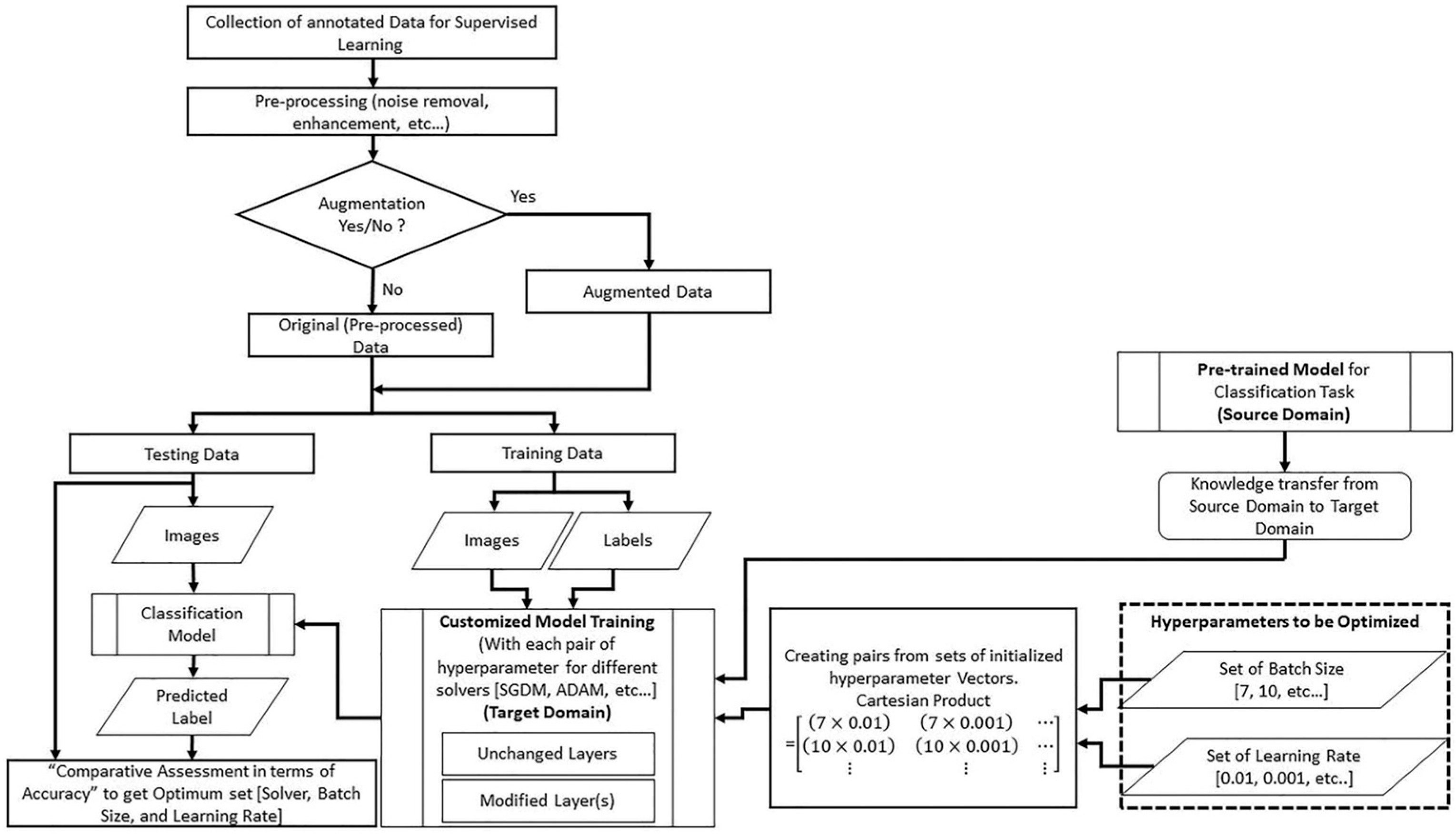
3.1. KBTL Implementation
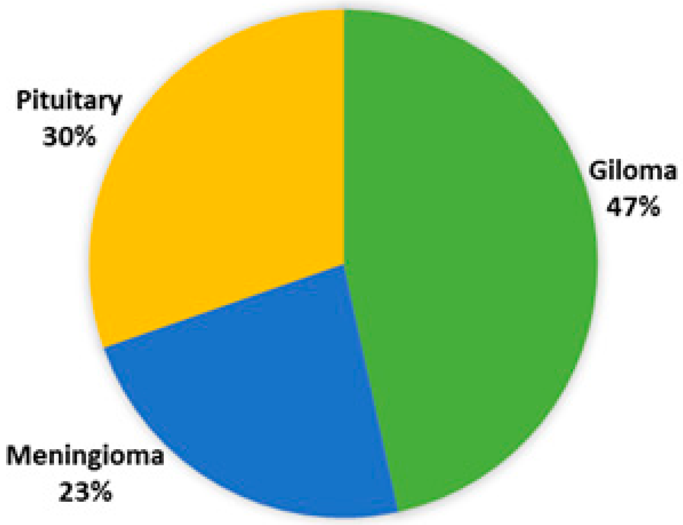
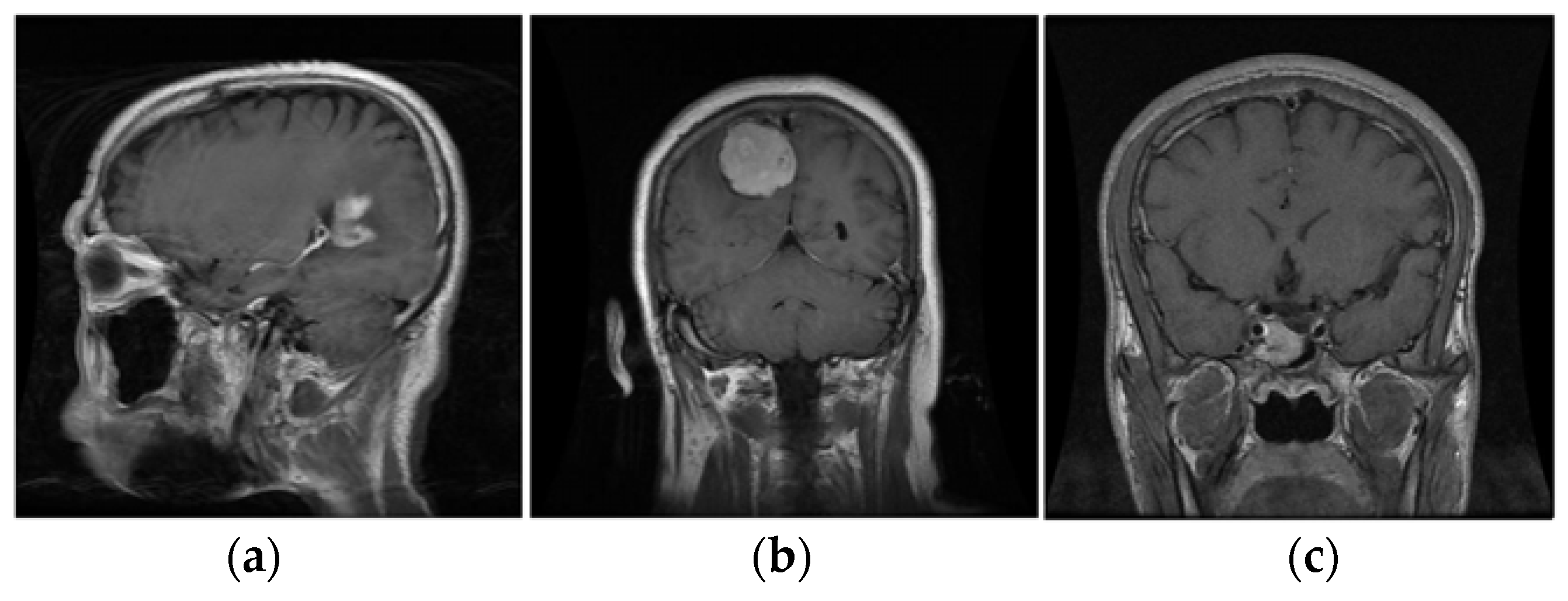
3.1.1. Dataset
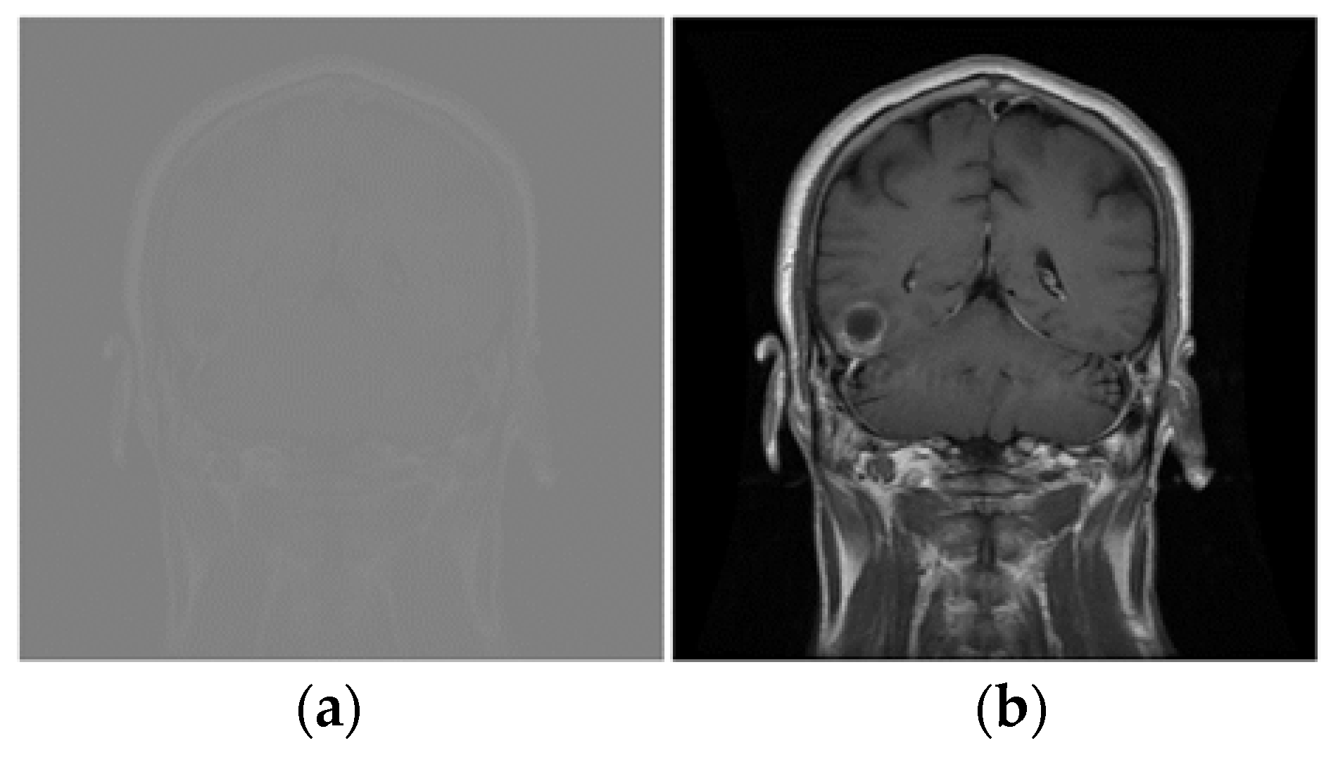
3.1.2. Preprocessing
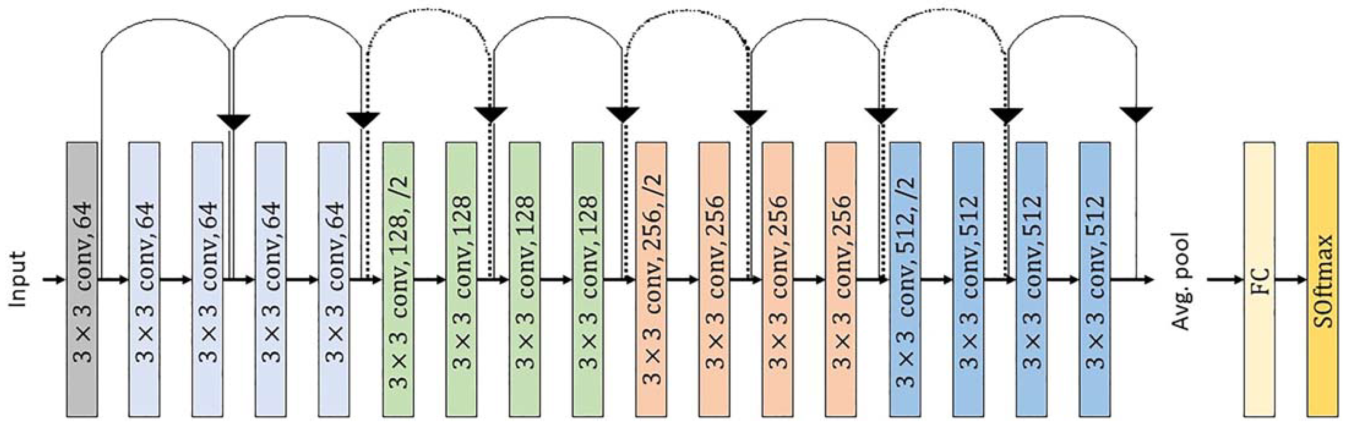
3.1.3. Pre-Trained DL Models
3.1.4. Model Training with Hyperparameters
3.2. Analysis of Variance (ANOVA)
3.2.1. Factor Effects Model
3.2.2. Estimates for the Factor Effects Model
3.2.3. Sum of Squares (SS) for ANOVA Table
3.2.4. Degree of Freedom (df) for ANOVA Table
3.2.5. Mean Square (MS) for ANOVA Table
3.2.6. Hypotheses for Two-Way ANOVA
3.2.7. F-Statistics for the Tests
4. Experimental Setup and Results Analysis
4.1. Simulated Results
4.2. Statistical Analysis
5. Conclusions and Future Work
Author Contributions
Funding
Data Availability Statement
Acknowledgments
Conflicts of Interest
References
- Selvanayaki, K.; Karnan, M. CAD system for automatic detection of brain tumor through magnetic resonance image-a review. Int. J. Eng. Sci. Technol. 2010, 2, 2. [Google Scholar]
- Brindle, K.M.; Izquierdo-García, J.L.; Lewis, D.Y.; Mair, R.J.; Wright, A.J. Brain Tumor Imaging. J. Clin. Oncol. 2017, 35, 2432–2438. [Google Scholar] [CrossRef] [PubMed] [Green Version]
- Wen, P.Y.; Macdonald, D.R.; Reardon, D.A.; Cloughesy, T.F.; Sorensen, A.G.; Galanis, E.; DeGroot, J.; Wick, W.; Gilbert, M.R.; Lassman, A.B.; et al. Updated Response Assessment Criteria for High-Grade Gliomas: Response Assessment in Neuro-Oncology Working Group. J. Clin. Oncol. 2010, 28, 1963–1972. [Google Scholar] [CrossRef]
- Drevelegas, A. Imaging of Brain Tumors with Histological Correlations; Springer: Berlin/Heidelberg, Germany, 2011; pp. 13–33. [Google Scholar]
- Cheng, J.; Huang, W.; Cao, S.; Yang, R.; Yang, W.; Yun, Z.; Wang, Z.; Feng, Q. Enhanced performance of brain tumor classification via tumor region augmentation and partition. PloS ONE 2015, 10, e0140381. [Google Scholar] [CrossRef] [PubMed]
- Cheng, J.; Yang, W.; Huang, M.; Huang, W.; Jiang, J.; Zhou, Y.; Yang, R.; Zhao, J.; Feng, Y.; Feng, Q.; et al. Retrieval of Brain Tumors by Adaptive Spatial Pooling and Fisher Vector Representation. PLoS ONE 2016, 11, e0157112. [Google Scholar] [CrossRef] [Green Version]
- Kumar, S.; Dabas, C.; Godara, S. Classification of Brain MRI Tumor Images: A Hybrid Approach. Procedia Comput. Sci. 2017, 122, 510–517. [Google Scholar] [CrossRef]
- Mohan, G.; Subashini, M.M. MRI based medical image analysis: Survey on brain tumor grade classification. Biomed. Signal Process. Control 2018, 39, 139–161. [Google Scholar] [CrossRef]
- Yang, F.; Zhang, W.; Tao, L.; Ma, J. Transfer Learning Strategies for Deep Learning-based PHM Algorithms. Appl. Sci. 2020, 10, 2361. [Google Scholar] [CrossRef] [Green Version]
- Usmani, I.A.; Qadri, M.T.; Zia, R.; Aziz, A.; Saeed, F. Cartesian Product Based Transfer Learning Implementation for Brain Tumor Classification. Comput. Mater. Contin. 2022, 73, 4369–4392. [Google Scholar] [CrossRef]
- Bahmani, M.; Shawi, R.E.; Potikyan, N.; Sakr, S. To tune or not to tune? An Approach for Recommending Important Hyperparameters. arXiv 2021, arXiv:2108.13066. [Google Scholar]
- He, K.; Zhang, X.; Ren, S.; Sun, J. Deep residual learning for image recognition. In Proceedings of the IEEE Conference on Computer Vision and Pattern Recognition, Las Vegas, NV, USA, 26 June–1 July 2016; pp. 770–778. [Google Scholar]
- Krizhevsky, A.; Sutskever, I.; Hinton, G.E. Imagenet classification with deep convolutional neural networks. Commun. ACM 2017, 60, 84–90. [Google Scholar] [CrossRef] [Green Version]
- Szegedy, C.; Liu, W.; Jia, Y.; Sermanet, P.; Reed, S.; Anguelov, D.; Erhan, D.; Vanhoucke, V.; Rabinovich, A. Going deeper with convolutions. In Proceedings of the IEEE Conference on Computer Vision and Pattern Recognition, Boston, MA, USA, 7–12 June 2015; pp. 1–9. [Google Scholar]
- Simonyan, K.; Zisserman, A. Very deep convolutional networks for large-scale image recognition. arXiv 2014, arXiv:1409.1556. [Google Scholar]
- Iandola, F.N.; Han, S.; Moskewicz, M.W.; Ashraf, K.; Dally, W.J.; Keutzer, K. SqueezeNet: AlexNet-level accuracy with 50x fewer parameters and <0.5 MB model size. arXiv 2016, arXiv:1602.07360. [Google Scholar]
- Sandler, M.; Howard, A.; Zhu, M.; Zhmoginov, A.; Chen, L.-C. Mobilenetv2: Inverted residuals and linear bottlenecks. In Proceedings of the IEEE Conference on Computer Vision and Pattern Recognition, Salt Lake City, UT, USA, 18–23 June 2018; pp. 4510–4520. [Google Scholar]
- Szegedy, C.; Vanhoucke, V.; Ioffe, S.; Shlens, J.; Wojna, Z. Rethinking the inception architecture for computer vision. In Proceedings of the IEEE Conference on Computer Vision and Pattern Recognition, Las Vegas, NV, USA, 27–30 June 2016; pp. 2818–2826. [Google Scholar]
- Radiuk, P.M. Impact of Training Set Batch Size on the Performance of Convolutional Neural Networks for Diverse Datasets. Inf. Technol. Manag. Sci. 2017, 20, 20–24. [Google Scholar] [CrossRef]
- Kandel, I.; Castelli, M. The effect of batch size on the generalizability of the convolutional neural networks on a histopathology dataset. ICT Express 2020, 6, 312–315. [Google Scholar] [CrossRef]
- Bengio, Y. Practical Recommendations for Gradient-Based Training of Deep Architectures. In Neural Networks: Tricks of the Trade; Springer: Berlin/Heidelberg, Germany, 2012; pp. 437–478. [Google Scholar]
- Masters, D.; Luschi, C. Revisiting small batch training for deep neural networks. arXiv 2018, arXiv:1804.07612. [Google Scholar]
- Russakovsky, O.; Deng, J.; Su, H.; Krause, J.; Satheesh, S.; Ma, S.; Huang, Z.; Karpathy, A.; Khosla, A.; Bernstein, M. Imagenet large scale visual recognition challenge. Int. J. Comput. Vis. 2015, 115, 211–252. [Google Scholar] [CrossRef] [Green Version]
- Krizhevsky, A.; Hinton, G. Learning Multiple Layers of Features from Tiny Images. 2009. Available online: http://www.cs.utoronto.ca/~kriz/learning-features-2009-TR.pdf (accessed on 7 January 2023).
- Cheng, J. Brain Tumor Dataset, Version 5. 2017. Available online: https://doi.org/10.6084/m9.figshare.1512427.v5 (accessed on 2 April 2017).
- Ramzan, F.; Khan, M.U.G.; Rehmat, A.; Iqbal, S.; Saba, T.; Rehman, A.; Mehmood, Z. A Deep Learning Approach for Automated Diagnosis and Multi-Class Classification of Alzheimer’s Disease Stages Using Resting-State fMRI and Residual Neural Networks. J. Med. Syst. 2019, 44, 37. [Google Scholar] [CrossRef]
- Yaqub, M.; Feng, J.; Zia, M.; Arshid, K.; Jia, K.; Rehman, Z.; Mehmood, A. State-of-the-Art CNN Optimizer for Brain Tumor Segmentation in Magnetic Resonance Images. Brain Sci. 2020, 10, 427. [Google Scholar] [CrossRef]
- Wu, S.; Hu, X.; Zheng, W.; He, C.; Zhang, G.; Zhang, H.; Wang, X. Effects of reservoir water level fluctuations and rainfall on a landslide by two-way ANOVA and K-means clustering. Bull. Eng. Geol. Environ. 2021, 80, 5405–5421. [Google Scholar] [CrossRef]
- Rouder, J.N.; Schnuerch, M.; Haaf, J.M.; Morey, R.D. Principles of Model Specification in ANOVA Designs. Comput. Brain Behav. 2022, 1–14. [Google Scholar] [CrossRef]
- Mahajan, R.; Kishore, K.; Jaswal, V. The challenges of interpreting ANOVA by dermatologists. Indian Dermatol. Online J. 2022, 13, 109. [Google Scholar] [CrossRef] [PubMed]
- Ismael, M.R.; Abdel-Qader, I. Brain tumor classification via statistical features and back-propagation neural network. In Proceedings of the 2018 IEEE International Conference on Electro/Information Technology (EIT), Rochester, MI, USA, 3–5 May 2018; pp. 0252–0257. [Google Scholar]
- Afshar, P.; Mohammadi, A.; Plataniotis, K.N. Brain tumor type classification via capsule networks. In Proceedings of the 2018 25th IEEE International Conference on Image Processing (ICIP), Athens, Greece, 7–10 October 2018; pp. 3129–3133. [Google Scholar]
- Pashaei, A.; Sajedi, H.; Jazayeri, N. Brain tumor classification via convolutional neural network and extreme learning machines. In Proceedings of the 2018 8th International Conference on Computer and Knowledge Engineering (ICCKE), Mashhad, Iran, 25–26 October 2018; pp. 314–319. [Google Scholar]
- Sajjad, M.; Khan, S.; Muhammad, K.; Wu, W.; Ullah, A.; Baik, S.W. Multi-grade brain tumor classification using deep CNN with extensive data augmentation. J. Comput. Sci. 2018, 30, 174–182. [Google Scholar] [CrossRef]
- Swati, Z.N.K.; Zhao, Q.; Kabir, M.; Ali, F.; Ali, Z.; Ahmed, S.; Lu, J. Brain tumor classification for MR images using transfer learning and fine-tuning. Comput. Med. Imaging Graph. 2019, 75, 34–46. [Google Scholar] [CrossRef] [PubMed]
- Deepak, S.; Ameer, P. Brain tumor classification using deep CNN features via transfer learning. Comput. Biol. Med. 2019, 111, 103345. [Google Scholar] [CrossRef] [PubMed]
- Muhammad, K.; Khan, S.; Del Ser, J.; de Albuquerque, V.H.C. Deep Learning for Multigrade Brain Tumor Classification in Smart Healthcare Systems: A Prospective Survey. IEEE Trans. Neural Netw. Learn. Syst. 2020, 32, 507–522. [Google Scholar] [CrossRef]
- Noreen, N.; Palaniappan, S.; Qayyum, A.; Ahmad, I.; Imran, M.; Shoaib, M. A Deep Learning Model Based on Concatenation Approach for the Diagnosis of Brain Tumor. IEEE Access 2020, 8, 55135–55144. [Google Scholar] [CrossRef]
- Sekhar, A.; Biswas, S.; Hazra, R.; Sunaniya, A.K.; Mukherjee, A.; Yang, L. Brain Tumor Classification Using Fine-Tuned GoogLeNet Features and Machine Learning Algorithms: IoMT Enabled CAD System. IEEE J. Biomed. Health Inform. 2021, 26, 983–991. [Google Scholar] [CrossRef]
- Rehman, A.; Naz, S.; Razzak, M.I.; Akram, F.; Imran, M. A Deep Learning-Based Framework for Automatic Brain Tumors Classification Using Transfer Learning. Circuits Syst. Signal Process. 2020, 39, 757–775. [Google Scholar] [CrossRef]


| Source | SS | df | MS | F |
|---|---|---|---|---|
| Columns (LR) | SS (LR) | |||
| Rows (BS) | SS (BS) | |||
| Interaction (LR × BS) | SS (LR × BS) | |||
| Error | SS (E) | |||
| Total | SS (total) |
| Pre-Trained Model | Confusion Matrix | Predicted Class | Solver | Batch Size | Learning Rate | Epoch | Validation Accuracy (%) | Testing Accuracy (%) | Training Time | |||
|---|---|---|---|---|---|---|---|---|---|---|---|---|
| G | M | P | ||||||||||
| AlexNet | True Class | G | 210 | 3 | 1 | SGDM | 32 | 0.001 | 54 | 97.17 | 97.6 | 0:14:44 |
| M | 2 | 101 | 3 | |||||||||
| P | 0 | 2 | 137 | |||||||||
| GoogleNet (ImageNet) | True Class | G | 210 | 4 | 0 | Adam | 10 | 0.0001 | 16 | 98.4 | 97.39 | 00:16:03 |
| M | 2 | 101 | 3 | |||||||||
| P | 1 | 2 | 136 | |||||||||
| GoogleNet (Places365) | True Class | G | 210 | 4 | 0 | SGDM | 10 | 0.001 | 20 | 98.26 | 97.17 | 00:14:42 |
| M | 6 | 99 | 1 | |||||||||
| P | 1 | 1 | 137 | |||||||||
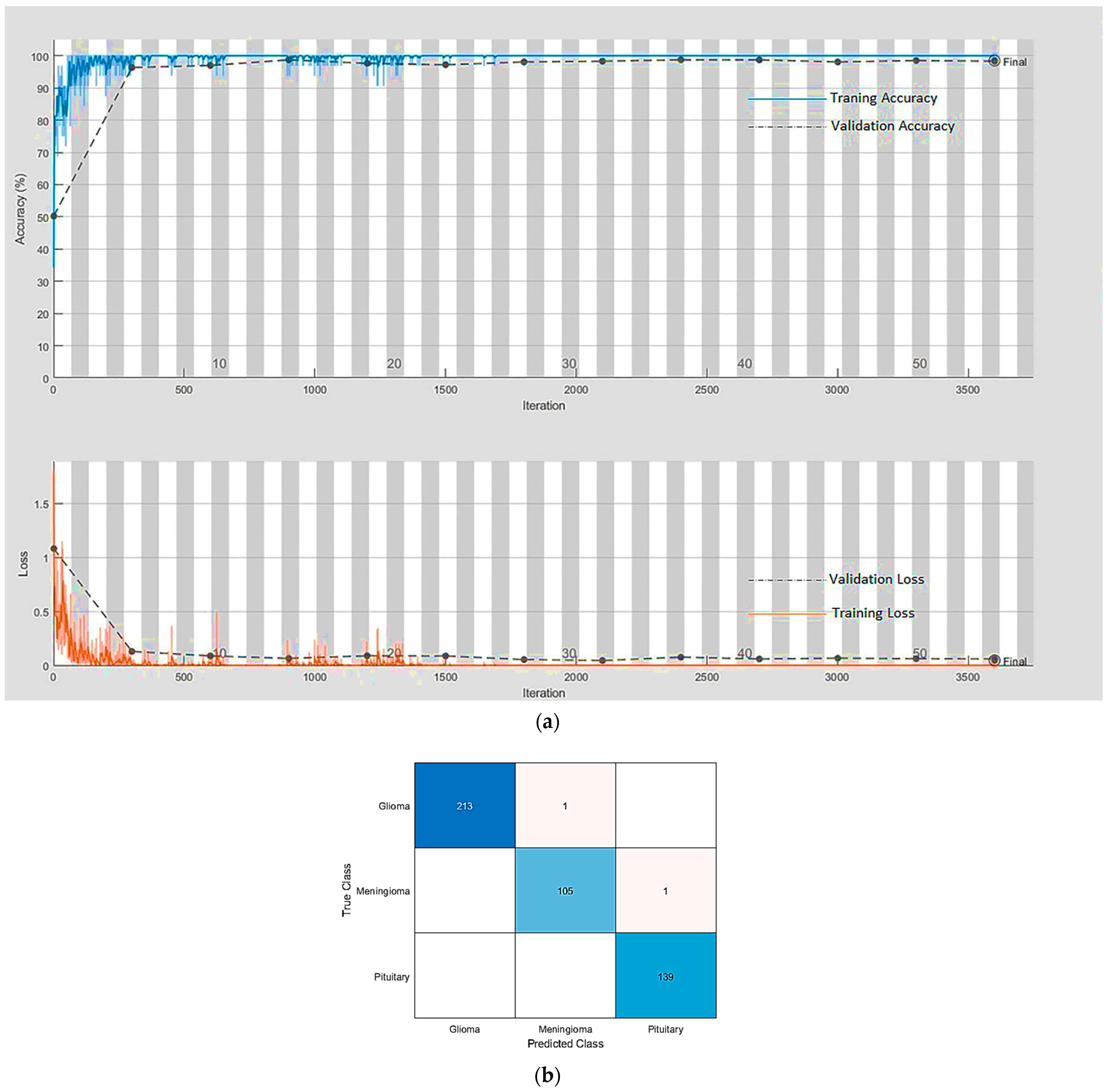
| ResNet-50 | True Class | G | 213 | 1 | 0 | SGDM | 7 | 0.001 | 17 | 98.26 | 99.56 | 0:24:46 |
| M | 1 | 105 | 0 | |||||||||
| P | 0 | 0 | 139 | |||||||||
| ResNet-101 | True Class | G | 213 | 1 | 0 | SGDM | 10 | 0.001 | 23 | 98.26 | 99.35 | 0:51:04 |
| M | 1 | 105 | 0 | |||||||||
| P | 1 | 0 | 138 | |||||||||
| ResNet-18 | True Class | G | 213 | 1 | 0 | SGDM | 32 | 0.01 | 54 | 98.48 | 99.56 | 0:19:25 |
| M | 0 | 105 | 1 | |||||||||
| P | 0 | 0 | 139 | |||||||||
| VGG16 | True Class | G | 214 | 0 | 0 | SGDM | 7 | 0.0001 | 11 | 96.74 | 98.26 | 0:14:41 |
| M | 6 | 98 | 2 | |||||||||
| P | 0 | 0 | 139 | |||||||||
| VGG19 | True Class | G | 211 | 3 | 0 | SGDM | 7 | 0.0001 | 15 | 97.17 | 98.69 | 0:21:24 |
| M | 1 | 105 | 0 | |||||||||
| P | 0 | 2 | 137 | |||||||||
| SqueezeNet | True Class | G | 208 | 5 | 1 | SGDM | 32 | 0.001 | 36 | 97.39 | 97.39 | 0:11:18 |
| M | 1 | 103 | 2 | |||||||||
| P | 2 | 1 | 136 | |||||||||
| MobileNet | True Class | G | 213 | 1 | 0 | SGDM | 32 | 0.01 | 54 | 97.61 | 98.91 | 0:43:46 |
| M | 1 | 103 | 2 | |||||||||
| P | 0 | 1 | 138 | |||||||||
| Inception V3 | True Class | G | 211 | 3 | 0 | RMS-Prop | 10 | 0.0001 | 20 | 98.04 | 98.26 | 0:58:39 |
| M | 1 | 103 | 2 | |||||||||
| P | 1 | 1 | 137 | |||||||||
| Fine-Tune Models | Precision Per Class | Average Precision | Sensitivity Per Class | Average Sensitivity | Specificity Per Class | Average Specificity |
|---|---|---|---|---|---|---|
| AlexNet | 99.06% | 97.61% | 98.13% | 97.60% | 99.18% | 98.91% |
| 95.28% | 95.28% | 98.58% | ||||
| 97.16% | 98.56% | 98.75% | ||||
| GoogleNet (ImageNet) | 98.11% | 96.97% | 97.20% | 96.95% | 98.37% | 98.53% |
| 92.59% | 94.34% | 97.73% | ||||
| 98.56% | 98.56% | 99.38% | ||||
| GoogleNet (Places365) | 96.77% | 97.17% | 98.13% | 97.17% | 97.14% | 98.25% |
| 95.19% | 93.40% | 98.58% | ||||
| 99.28% | 98.56% | 99.69% | ||||
| ResNet50 | 99.53% | 99.56% | 99.53% | 99.56% | 99.59% | 99.74% |
| 99.06% | 99.06% | 99.72% | ||||
| 100.00% | 100.00% | 100.00% | ||||
| ResNet101 | 99.07% | 99.35% | 99.53% | 99.35% | 99.18% | 99.55% |
| 99.06% | 99.06% | 99.72% | ||||
| 100.00% | 99.28% | 100.00% | ||||
| ResNet18 | 100.00% | 99.57% | 99.53% | 99.56% | 100.00% | 99.84% |
| 99.06% | 99.06% | 99.72% | ||||
| 99.29% | 100.00% | 99.69% | ||||
| VGG16 | 97.27% | 98.30% | 100.00% | 98.26% | 97.55% | 98.67% |
| 100.00% | 92.45% | 100.00% | ||||
| 98.58% | 100.00% | 99.38% | ||||
| VGG19 | 99.53% | 98.73% | 98.60% | 98.69% | 99.59% | 99.48% |
| 95.45% | 99.06% | 98.58% | ||||
| 100.00% | 98.56% | 100.00% | ||||
| SqueezeNet | 98.58% | 97.41% | 97.20% | 97.39% | 98.78% | 98.75% |
| 94.50% | 97.17% | 98.30% | ||||
| 97.84% | 97.84% | 99.06% | ||||
| MobileNet | 99.53% | 98.91% | 99.53% | 98.91% | 99.59% | 99.49% |
| 98.10% | 97.17% | 99.43% | ||||
| 98.57% | 99.28% | 99.38% | ||||
| InceptionV3 | 99.06% | 98.26% | 98.60% | 98.26% | 99.18% | 99.17% |
| 96.26% | 97.17% | 98.87% | ||||
| 98.56% | 98.56% | 99.38% |
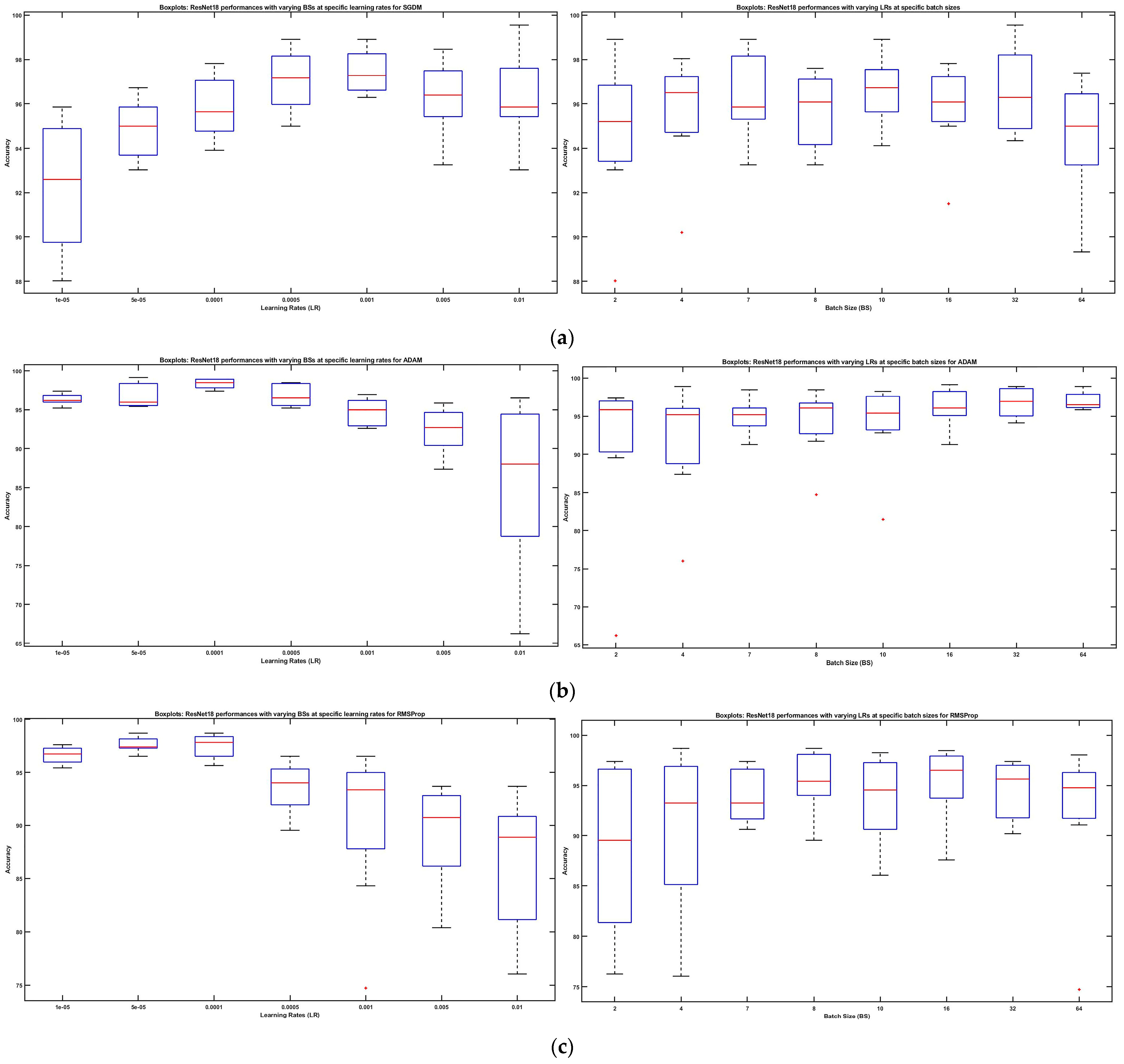
| ResNet18 | ResNet50 | ResNet101 | ||||||||||||||||||||
|---|---|---|---|---|---|---|---|---|---|---|---|---|---|---|---|---|---|---|---|---|---|---|
| SGDM | SGDM | SGDM | ||||||||||||||||||||
| LR | 0.01 | 0.005 | 0.001 | 5 × 10⁻⁴ | 1 × 10⁻⁴ | 5 × 10⁻⁵ | 1 × 10⁻⁵ | 0.01 | 0.005 | 0.001 | 5 × 10⁻⁴ | 1 × 10⁻⁴ | 5 × 10⁻⁵ | 1 × 10⁻⁵ | 0.01 | 0.005 | 0.001 | 5 × 10⁻⁴ | 1 × 10⁻⁴ | 5 × 10⁻⁵ | 1 × 10⁻⁵ | |
| BS | ||||||||||||||||||||||
| 2 | 93.03 | 94.55 | 97.17 | 98.91 | 95.21 | 95.86 | 88.02 | 92.59 | 94.99 | 96.95 | 98.26 | 95.86 | 96.73 | 92.16 | 78.87 | 94.77 | 96.08 | 97.6 | 95.64 | 94.77 | 89.76 | |
| 4 | 95.21 | 96.51 | 97.39 | 98.04 | 94.55 | 96.73 | 90.2 | 96.95 | 94.99 | 98.04 | 98.69 | 96.08 | 96.73 | 94.12 | 97.6 | 97.82 | 97.82 | 97.6 | 95.42 | 94.12 | 93.9 | |
| 7 | 95.64 | 93.25 | 98.91 | 98.26 | 97.82 | 95.21 | 95.86 | 96.73 | 98.04 | 99.56 | 97.82 | 97.17 | 97.17 | 95.21 | 98.69 | 98.04 | 97.82 | 98.26 | 97.17 | 95.42 | 95.86 | |
| 8 | 95.64 | 97.17 | 97.6 | 96.95 | 96.08 | 93.25 | 93.68 | 97.17 | 96.73 | 98.26 | 97.82 | 95.64 | 95.86 | 95.64 | 97.6 | 98.91 | 98.69 | 97.39 | 96.3 | 95.21 | 93.03 | |
| 10 | 97.82 | 96.3 | 98.91 | 96.73 | 96.73 | 94.12 | 95.42 | 97.6 | 98.26 | 99.35 | 97.17 | 96.95 | 96.08 | 96.3 | 98.04 | 97.17 | 99.35 | 98.91 | 96.73 | 95.42 | 94.34 | |
| 16 | 96.08 | 97.82 | 96.73 | 97.39 | 94.99 | 95.86 | 91.5 | 98.69 | 98.04 | 98.04 | 96.95 | 95.42 | 97.17 | 91.94 | 98.04 | 98.69 | 98.04 | 97.82 | 96.08 | 95.64 | 93.25 | |
| 32 | 99.56 | 98.47 | 96.3 | 95.21 | 97.39 | 94.77 | 94.34 | 97.39 | 96.73 | 97.82 | 96.95 | 95.86 | 94.99 | 92.37 | 98.69 | 98.47 | 95.64 | 96.3 | 95.21 | 94.12 | 93.9 | |
| 64 | 97.39 | 96.3 | 96.51 | 94.99 | 93.9 | 93.03 | 89.32 | 97.17 | 96.51 | 94.77 | 96.3 | 95.42 | 96.3 | 89.54 | 97.6 | 98.04 | 95.17 | 95.82 | 95.04 | 92.37 | 92.16 | |
| ADAM | ADAM | ADAM | ||||||||||||||||||||
| 2 | 66.23 | 89.54 | 92.59 | 95.86 | 97.39 | 95.86 | 97.39 | 68.63 | 76.47 | 90.58 | 96.51 | 97.82 | 96.95 | 95.86 | 62.96 | 79.08 | 65.58 | 90.41 | 97.17 | 94.99 | 91.29 | |
| 4 | 76.03 | 87.36 | 93.03 | 95.21 | 98.91 | 96.08 | 95.86 | 69.72 | 88.89 | 93.9 | 92.16 | 96.51 | 95.42 | 96.95 | 71.68 | 86.06 | 93.9 | 89.76 | 97.39 | 97.82 | 98.26 | |
| 7 | 91.29 | 93.68 | 93.9 | 95.21 | 98.47 | 95.42 | 96.3 | 80.61 | 83.22 | 96.08 | 97.39 | 98.26 | 98.47 | 94.99 | 79.74 | 88.24 | 92.37 | 96.95 | 97.39 | 97.39 | 96.73 | |
| 8 | 84.75 | 91.72 | 96.08 | 96.95 | 98.47 | 95.64 | 96.08 | 78.43 | 94.55 | 94.55 | 91.29 | 97.82 | 98.91 | 96.73 | 84.1 | 84.97 | 93.25 | 97.6 | 99.13 | 97.17 | 95.64 | |
| 10 | 81.48 | 94.34 | 92.81 | 98.26 | 98.04 | 95.42 | 96.3 | 90.41 | 94.55 | 95.64 | 95.21 | 98.26 | 97.39 | 95.42 | 88.45 | 92.81 | 92.59 | 95.86 | 97.17 | 97.6 | 96.73 | |
| 16 | 94.77 | 91.29 | 96.08 | 98.47 | 97.6 | 99.13 | 96.08 | 91.72 | 92.59 | 95.21 | 97.17 | 99.13 | 98.91 | 96.3 | 83.01 | 90.2 | 94.77 | 97.17 | 98.47 | 96.3 | 94.34 | |
| 32 | 94.12 | 94.99 | 96.95 | 98.47 | 98.91 | 98.69 | 95.21 | 87.58 | 95.21 | 96.51 | 98.04 | 97.17 | 98.91 | 96.08 | 93.46 | 91.7 | 91.29 | 96.51 | 97.82 | 97.6 | 95.64 | |
| 64 | 96.51 | 95.86 | 96.3 | 96.08 | 98.91 | 98.04 | 97.39 | 92.16 | 95.86 | 95.21 | 95.64 | 98.26 | 98.91 | 93.9 | 90.63 | 90.81 | 91.7 | 95.21 | 97.39 | 96.51 | 93.04 | |
| RMSProp | RMSProp | RMSProp | ||||||||||||||||||||
| 2 | 76.25 | 80.39 | 84.31 | 89.54 | 95.64 | 97.39 | 96.95 | 64.71 | 81.92 | 85.4 | 83.88 | 98.26 | 96.51 | 96.95 | 23.09 | 64.92 | 82.79 | 79.96 | 96.73 | 98.04 | 94.12 | |
| 4 | 76.03 | 82.79 | 92.16 | 93.25 | 98.69 | 97.39 | 95.42 | 78.65 | 87.15 | 92.16 | 93.25 | 98.47 | 97.82 | 98.04 | 78.43 | 84.53 | 89.32 | 94.12 | 98.04 | 98.91 | 95.64 | |
| 7 | 90.63 | 92.81 | 91.29 | 93.25 | 95.64 | 97.39 | 96.95 | 76.47 | 88.24 | 88.45 | 97.82 | 98.91 | 97.17 | 95.42 | 79.3 | 81.05 | 90.41 | 95.42 | 96.51 | 98.04 | 96.08 | |
| 8 | 93.68 | 89.54 | 95.42 | 94.99 | 98.26 | 98.69 | 97.6 | 85.84 | 82.35 | 91.5 | 96.95 | 98.04 | 97.6 | 98.26 | 86.71 | 87.58 | 91.72 | 94.55 | 98.04 | 98.47 | 95.64 | |
| 10 | 86.06 | 90.63 | 94.55 | 90.63 | 97.6 | 98.26 | 96.3 | 86.93 | 89.98 | 92.75 | 94.99 | 96.73 | 98.69 | 96.73 | 89.11 | 91.5 | 94.34 | 94.34 | 98.47 | 97.6 | 97.6 | |
| 16 | 87.58 | 92.81 | 96.51 | 96.51 | 98.47 | 98.04 | 97.6 | 83.22 | 89.54 | 93.03 | 97.39 | 97.17 | 98.47 | 95.86 | 83.66 | 91.29 | 93.9 | 93.03 | 96.3 | 97.82 | 96.73 | |
| 32 | 90.2 | 90.85 | 94.55 | 95.64 | 97.39 | 97.17 | 96.51 | 88.89 | 91.94 | 94.77 | 91.07 | 97.82 | 98.91 | 96.51 | 85.19 | 90.72 | 97.17 | 95.64 | 97.82 | 98.04 | 96.8 | |
| 64 | 91.07 | 93.68 | 74.73 | 94.77 | 98.04 | 96.51 | 95.64 | 91.5 | 89.98 | 95.86 | 96.51 | 97.39 | 98.26 | 94.77 | 80.61 | 88.89 | 94.55 | 93.9 | 95.21 | 97.39 | 95.86 | |
| Related Work | Approach | Accuracy | Precision | Recall | Specificity | |||||||||
|---|---|---|---|---|---|---|---|---|---|---|---|---|---|---|
| G | M | P | Average | G | M | P | Average | G | M | P | Average | |||
| [5] | BoW-SVM | 91.28 | - | - | - | - | 96.4 | 86 | 87.3 | - | 96.3 | 95.5 | 95.3 | - |
| [31] | DWT-Gabor-NN | 91.90 | - | - | - | - | 95.1 | 86.9 | 91.2 | - | 96.3 | 96 | 95.7 | - |
| [32] | CapsNet | 90.89 | - | - | - | - | - | - | - | - | - | - | - | - |
| [33] | CNN-ELM | 93.68 | 91 | 94.5 | 98.3 | - | 97.5 | 76.8 | 100 | - | - | - | - | - |
| [34] | VGG19 | 94.58 | - | - | - | - | - | - | - | 88.41 | - | - | - | 96.12 |
| [35] | VGG19 | 94.82 | 93 | 87.97 | 87.34 | 89.52 | 95.97 | 89.98 | 96.81 | 94.25 | 93.79 | 96.42 | 93.93 | 94.69 |
| [36] | GoogleNet-SVM | 97.10 | 99 | 94.7 | 98 | - | 97.9 | 96 | 98.9 | - | 99.4 | 98.4 | 99.1 | - |
| [40] | VGG16 | 98.69 | - | - | - | - | - | - | - | - | - | - | - | - |
| [37] | VGGNet | 94.00 | - | - | - | - | - | - | - | - | - | - | - | - |
| [38] | DenseNet | 99.51 | 99 | 99 | 100 | - | 100 | 99 | 99 | - | - | - | - | - |
| [39] | GoogleNet-KNN | 98.30 | 98 | 95.55 | 97.78 | - | 98.02 | 94.57 | 99.1 | - | 98.63 | 98.65 | 99.01 | - |
| Our Approach | ResNet18 | 99.56 | 100 | 99.06 | 99.29 | 99.45 | 99.53 | 99.06 | 100 | 99.53 | 100 | 99.72 | 99.69 | 99.8 |
| LR BS | 0.01 | 0.005 | 0.001 | 0.0005 | 0.0001 | 0.00005 | 0.00001 |
|---|---|---|---|---|---|---|---|
| 2 | 93.03 | 94.55 | 97.17 | 98.91 | 95.21 | 95.86 | 88.02 |
| 92.59 | 94.99 | 96.95 | 98.26 | 95.86 | 96.73 | 92.16 | |
| 78.87 | 94.77 | 96.08 | 97.60 | 95.64 | 94.77 | 89.76 | |
| 4 | 95.21 | 96.51 | 97.39 | 98.04 | 94.55 | 96.73 | 90.20 |
| 96.95 | 94.99 | 98.04 | 98.69 | 96.08 | 96.73 | 94.12 | |
| 97.60 | 97.82 | 97.82 | 97.60 | 95.42 | 94.12 | 93.90 |
| Source | SS | df | MS | F | Prob > F |
|---|---|---|---|---|---|
| LRs | 367.89 | 6 | 61.3145 | 27.91 | 3.52524 × 10⁻²⁰ |
| BSs | 148.04 | 7 | 21.148 | 9.63 | 2.4884 × 10⁻⁹ |
| Interaction | 292.94 | 42 | 6.9748 | 3.17 | 6.57531 × 10⁻⁷ |
| Error | 246.07 | 112 | 2.1971 | ||
| Total | 1054.94 | 167 |
| Group A | Group B | Lower Limit | A-B | Upper Limit | p-Value |
|---|---|---|---|---|---|
| 1 | 2 | −1.9294 | −0.64458 | 0.6402 | 0.74045 |
| 1 | 3 | −2.5744 | −1.2896 | −0.0047974 | 0.048506 |
| 1 | 4 | −2.4115 | −1.1267 | 0.15812 | 0.12605 |
| 1 | 5 | −1.0219 | 0.26292 | 1.5477 | 0.99624 |
| 1 | 6 | −0.44145 | 0.84333 | 2.1281 | 0.43887 |
| 1 | 7 | 2.1056 | 3.3904 | 4.6752 | 3.71 × 10⁻⁸ |
| 2 | 3 | −1.9298 | −0.645 | 0.63979 | 0.73987 |
| 2 | 4 | −1.7669 | −0.48208 | 0.8027 | 0.9186 |
| 2 | 5 | −0.37729 | 0.9075 | 2.1923 | 0.34781 |
| 2 | 6 | 0.20313 | 1.4879 | 2.7727 | 0.01243 |
| 2 | 7 | 2.7502 | 4.035 | 5.3198 | 3.71 × 10⁻⁸ |
| 3 | 4 | −1.1219 | 0.16292 | 1.4477 | 0.99975 |
| 3 | 5 | 0.26771 | 1.5525 | 2.8373 | 0.0076499 |
| 3 | 6 | 0.84813 | 2.1329 | 3.4177 | 4.61 × 10⁻⁵ |
| 3 | 7 | 3.3952 | 4.68 | 5.9648 | 3.71 × 10⁻⁸ |
| 4 | 5 | 0.1048 | 1.3896 | 2.6744 | 0.025044 |
| 4 | 6 | 0.68521 | 1.97 | 3.2548 | 0.00021833 |
| 4 | 7 | 3.2323 | 4.5171 | 5.8019 | 3.71 × 10⁻⁸ |
| 5 | 6 | −0.70437 | 0.58042 | 1.8652 | 0.82336 |
| 5 | 7 | 1.8427 | 3.1275 | 4.4123 | 3.79 × 10⁻⁸ |
| 6 | 7 | 1.2623 | 2.5471 | 3.8319 | 6.74 × 10⁻⁷ |
| Group A | Group B | Lower Limit | A-B | Upper Limit | p-Value |
|---|---|---|---|---|---|
| 1 | 2 | −3.3525 | −1.9395 | −0.5265 | 0.0012 |
| 1 | 3 | −4.2764 | −2.8633 | −1.4503 | 2.6014 × 10⁻⁷ |
| 1 | 4 | −3.6435 | −2.2305 | −0.8175 | 9.5937 × 10⁻⁵ |
| 1 | 5 | −4.2664 | −2.8533 | −1.4403 | 2.8206 × 10⁻⁷ |
| 1 | 6 | −3.6225 | −2.2095 | −0.7965 | 1.1579 × 10⁻⁴ |
| 1 | 7 | −3.4464 | −2.0333 | −0.6203 | 5.3643 × 10⁻⁴ |
| 1 | 8 | −2.1325 | −0.7195 | 0.6935 | 0.7653 |
| 2 | 3 | −2.3368 | −0.9238 | 0.4892 | 0.4736 |
| 2 | 4 | −1.7040 | −0.2910 | 1.1221 | 0.9983 |
| 2 | 5 | −2.3268 | −0.9138 | 0.4992 | 0.4881 |
| 2 | 6 | −1.6830 | −0.2700 | 1.1430 | 0.9989 |
| 2 | 7 | −1.5068 | −0.0938 | 1.3192 | 1.0000 |
| 2 | 8 | −0.1930 | 1.2200 | 2.6330 | 0.1439 |
| 3 | 4 | −0.7802 | 0.6329 | 2.0459 | 0.8629 |
| 3 | 5 | −1.4030 | 0.0100 | 1.4230 | 1.0000 |
| 3 | 6 | −0.7592 | 0.6538 | 2.0668 | 0.8418 |
| 3 | 7 | −0.5830 | 0.8300 | 2.2430 | 0.6117 |
| 3 | 8 | 0.7308 | 2.1438 | 3.5568 | 2.0727 × 10⁻⁴ |
| 4 | 5 | −2.0359 | −0.6229 | 0.7902 | 0.8724 |
| 4 | 6 | −1.3921 | 0.0210 | 1.4340 | 1.0000 |
| 4 | 7 | −1.2159 | 0.1971 | 1.6102 | 0.9999 |
| 4 | 8 | 0.0979 | 1.5110 | 2.9240 | 0.0272 |
| 5 | 6 | −0.7692 | 0.6438 | 2.0568 | 0.8521 |
| 5 | 7 | −0.5930 | 0.8200 | 2.2330 | 0.6264 |
| 5 | 8 | 0.7208 | 2.1338 | 3.5468 | 2.2624 × 10⁻⁴ |
| 6 | 7 | −1.2368 | 0.1762 | 1.5892 | 0.9999 |
| 6 | 8 | 0.0770 | 1.4900 | 2.9030 | 0.0311 |
| 7 | 8 | −0.0992 | 1.3138 | 2.7268 | 0.0883 |
Disclaimer/Publisher’s Note: The statements, opinions and data contained in all publications are solely those of the individual author(s) and contributor(s) and not of MDPI and/or the editor(s). MDPI and/or the editor(s) disclaim responsibility for any injury to people or property resulting from any ideas, methods, instructions or products referred to in the content. |
© 2023 by the authors. Licensee MDPI, Basel, Switzerland. This article is an open access article distributed under the terms and conditions of the Creative Commons Attribution (CC BY) license (https://creativecommons.org/licenses/by/4.0/).
Share and Cite
Usmani, I.A.; Qadri, M.T.; Zia, R.; Alrayes, F.S.; Saidani, O.; Dashtipour, K. Interactive Effect of Learning Rate and Batch Size to Implement Transfer Learning for Brain Tumor Classification. Electronics 2023, 12, 964. https://doi.org/10.3390/electronics12040964
Usmani IA, Qadri MT, Zia R, Alrayes FS, Saidani O, Dashtipour K. Interactive Effect of Learning Rate and Batch Size to Implement Transfer Learning for Brain Tumor Classification. Electronics. 2023; 12(4):964. https://doi.org/10.3390/electronics12040964
Chicago/Turabian StyleUsmani, Irfan Ahmed, Muhammad Tahir Qadri, Razia Zia, Fatma S. Alrayes, Oumaima Saidani, and Kia Dashtipour. 2023. "Interactive Effect of Learning Rate and Batch Size to Implement Transfer Learning for Brain Tumor Classification" Electronics 12, no. 4: 964. https://doi.org/10.3390/electronics12040964