
Research on Extended Target-Tracking Algorithms of Sea Surface Navigation Radar


College of Communication and Information Engineering, Xi’an University of Science and Technology, Xi’an 710054, China
*
Author to whom correspondence should be addressed.
Electronics 2023, 12(3), 616; https://doi.org/10.3390/electronics12030616
Submission received: 16 December 2022
/
Revised: 20 January 2023
/
Accepted: 24 January 2023
/
Published: 26 January 2023
(This article belongs to the Special Issue Advances in Radar Imaging and Target Tracking)
Abstract
:To solve the problem of false tracks generated by breakdowns and clutter in point-target tracking in polar coordinates, a fusion tracking algorithm based on a converted measurement Kalman filter and random matrix expansion is proposed. The converted measurement Kalman filter (CMKF) transforms the polar coordinate data of the target at the current time into Cartesian coordinates without bias. Based on linear measurements and states, the position of the extended target and the group target was predicted and updated by using a random matrix, and its track was drawn by combining the nearest neighbors to realize the tracking of the size, shape and azimuth of the extended target. Compared with point-target tracking, the accuracy of extended multi-target tracking was increased by 45.8% based on data measured using NAVICO navigation radar aboard ships at sea. The experimental results showed that the improved method in this paper could effectively reduce the interference of clutter on target tracking and provide more information about the target motion features.
1. Introduction
One of the primary methods for ensuring the security of ship navigation and the management of maritime traffic is target tracking by navigation radar. As a measuring tool, radar measurement data contain some mistakes, which, when combined with the noise produced by various external factors and sea surface weather, lead to missed and false tracks in multi-target tracking, lowering the statistical accuracy of the ship’s flow. For improved safety of ship navigation and the management of sea area traffic, reliable target tracking is therefore crucial.
Modern marine navigation radar is widely used in the military and the transportation sector. Traditional tracking theories assume the target is a point source when estimating the state of the target (i.e., position, velocity and acceleration), resulting in the size, shape and azimuth of the target being ignored. However, with the continuous improvement in the resolution of sensors, this assumption is no longer valid. In marine surveillance, different scattering centers of the observed objects may lead to multiple measurements. If the point target is still used for tracking, the tracking accuracy will be reduced and the navigation system may be broken down. In addition, modern applications need more detailed physical information about target objects to detect, track, classify and identify them, etc. In this case, the detection object is generally regarded as an extended target with a size, shape and azimuth [1,2,3,4]. Multi-target tracking also faces similar challenges. The direction of multi-target tracking is conducive to practical applications, such as identifying the classification and movement direction of ships at sea. Therefore, more attention should be paid to the kinematic information of group targets in the extension of multi-target tracking.
At present, many traditional algorithms are applied in multi-target tracking, such as Group Probabilistic Data Association (GPDA), the Multi-hypothesis Tracking Algorithm (MHT), particle filtering, etc. In order to improve the accuracy of multi-target tracking, changes would have to be made to these algorithms, which is difficult. A rough Bayesian solution to the extended target tracking problem is offered in Koch’s [4] extended target and group target tracking (ETT and GTT) model, which is predicated on the assumption of elliptical targets. The expanded spherical object is represented by random matrices, the goal motion state by a Gaussian distribution, and the ellipsoidal expansion by an inverse Wishart distribution. One benefit is that the extended object or target group is viewed as a tracking object since it can estimate the target’s state of motion and physical expansion. In order to address several of the shortcomings in [5], such as sensor failures not being taken into account in the initial framework, a new random matrix approach is inferred in [3]. In reality, as explained in [3], which provides an approach to integrate the random matrix and the interactive multiple model estimator, if the sensor noise is greater than the goal size, the lack of modeling may result in an overestimation of the target size [4]. While target locations and dynamics are often represented in Cartesian coordinates, new measurements and time updates in [3] are supplied in Polar coordinates. Target tracking performance may be impacted if the impact the translation from polar to Cartesian coordinates has on the data is not correctly taken into account. For tracking extended target objects represented using the elliptical random hypersurface model, [6] uses a Random Hypersurface Model (RHM), providing new results and insights for expanding the target object. Ellipse RHM uses a one-dimensional random scale factor to specify the square Mahalanobis distance between the measurement source and the target object’s center. For situations with substantial measurement noise, an ellipse-shaped Bayesian inference method is also appropriate. In [7], a random matrix approach for extended object and group target tracking (EOT/GTT) based on nonlinear measurements is provided. Under some circumstances, linearized measurements can be easily transformed and incorporated into the current random matrix techniques. In [8], a more precise tracking method is used with unbiased uniform transformation measurements, which solves the problem of sensor’s inaccuracy related to the actual geometry and accuracy. Compared with the three Kalman filters, the calculation time of EKF is significantly lower than that of UF and PF. When the degree of nonlinearity of the research environment increases, the filtering effect of EKF will significantly decline or even diverge [9]. The Interacting Multiple Model Algorithm (IMM) has been applied to many tracking systems, but the performance of the algorithm depends too much on the model set it uses, which may increase the system’s computational cost [10]. Reference [11] presents a joint estimation method for the target state and an unknown input under the criterion of maximum correlation entropy to solve the problem of linearizing the tracking of moving targets in Cartesian coordinates with unbiased transformation measurements. The video resolution is improved through the video resolution enhancement module, then the local intensity and gradient (LIG) algorithm is also improved and applied to the frame-by-frame detection of small targets. Finally, Simple Online and Realtime Tracking (SORT) is used to realize the multi-target tracking association in videos [12]. The converted measurement noise satisfies a Gaussian distribution. Navigation radar returns two-dimensional measurements of data, where the target position is represented in polar coordinates at angles and distances. The inaccuracy of these measurements has a small impact on tracking performance, because the Cartesian coordinate system is the best way to model the target in target tracking. Therefore, polar data are processed using the following methods. One method is to use Kalman filter to filter the measurements in a Cartesian coordinate system; the other is to use a non-linear extended Kalman filter (EKF), which combines the original measurements into a target state estimation in a non-linear way, resulting in a mixed coordinate filter. In the first method, the transformed measurement covariance is recalculated in each recursion of the filter. In the second filter (EKF), the initial state covariance depends on the measurement accuracy of the initial transformation, the gain depends on the accuracy of subsequent linearization, and the overall filtering effect largely depends on the accuracy of both the above transformations.
This paper presents a fusion tracking algorithm to solve the problems of inaccurate conversion and poor clutter suppression. The Extended Target Kalman Filter algorithm after transforming measurements (CMKF-RMETT) was used to measure conversion preprocessing and random matrix expansion to track various ship targets at sea. Using the feedback of measurement information in a polar coordinate system, the CMKF algorithm introduced the error parameters of the radar in angle and measurement range. Based on the linear measurement of the unbiased conversion of radar, the algorithm used a random matrix to extend the tracking of the target. This method solves the problem of point target breakdown and spurious track formation during tracking and outputs the movement characteristic information of the target.
2. Materials and Methods
2.1. Target Data Collection
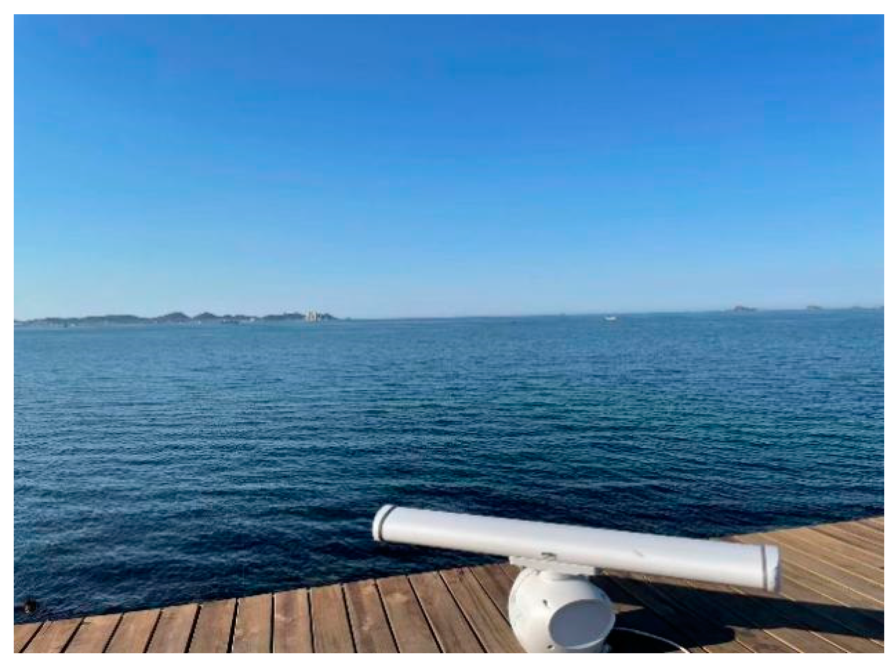
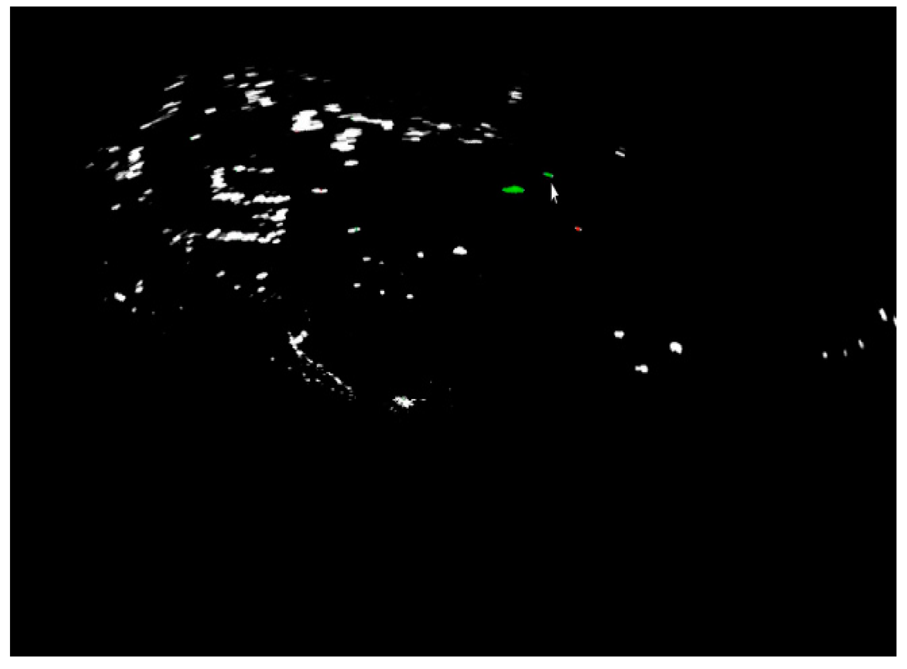
The experimental data were provided by the pulse navigation radar manufactured by NAVICO. The actual measurement and collection environment is shown in Figure 1. The experimental site is an area of the sea in Yantai. The radar is installed at the coastal position. The PPI imaging real-time video information provided by the radar system is used for auxiliary analysis. NAVICO’s pulse navigation radar collects data by using the system’s own SOPKE for sampling and reading. The radar sets the true north direction to rotate at an angle of 0 degrees (one rotation of the antenna is divided into 4096 deflection angles) for data sampling. The range resolution will automatically set appropriate parameters (distancecell) according to the distance of different targets from the radar. The longest distance of radar sampling is a 1024 times range resolution ( = distancecell × 1024). That is, in different scenes, the radar will use different parameters for the data sampling of the targets. Figure 2 and Figure 3 show the target feedback position information of a moving fishing boat in different scenarios. The radar will use different parameters to sample the data of the target. The figures depict the moving fishing boat detected by the radar in red and green ellipses. Partial system parameters and performance indices of the radar are shown in Table 1 below.
2.2. Point-Target Tracking Algorithm
The tracking algorithm adopted at the beginning of the study set the fishing boat as a point target for track, ignoring the size of the target. When the algorithm preprocesses the DBSCAN clustering [13], the angle and distance of coordinates were normalized to obtain the Euclidean distance to reduce the error. The center point of each cluster was selected as the target position, and the track is started by the logic method. Since the radar measurement has no return velocity value, the average velocity of the first three frames was obtained according to the different methods used to meet the conditions for creating the equation of motion. In the case the motion is highly nonlinear, the extended Kalman filter (EKF) was used and probabilistic data association (PDA) was used to judge the track.
2.3. Extended Target Tracking Algorithm
Most tracking applications consider the target as a point source for measurement. By estimating the motion state of the target, ignoring details including size, shape and orientation, the problem can be simplified due to the practical limitations and theoretical considerations. However, with the increase in the resolutions of modern sensors, the effectiveness of treating objects as point masses decreases. In this case, considering the object as an extended target with a size, shape and orientation can improve the accuracy of its tracking. In the context of the present high-precision sensors, researches have studied target extensions, providing a well-established and widely used ETT framework under the assumption of an ellipsoidal target shape, where an approximate Bayesian solution to the extended target tracking problem is proposed [14,15,16,17,18]. Ellipsoidal object extension is modeled using a random matrix and is considered as an additional state variable to be estimated. The target’s kinematic states are modeled using a Gaussian distribution, while the ellipsoidal target’s extension is modeled using an inverse Wishart distribution. The algorithm incorporating the above transformations presupposes an unbiased conversion of the radar measurements to a Cartesian coordinate system before the extended model, so that the measurements show a linear relationship with the target state for a more accurate update of the true position of the target by the subsequent random matrix [19,20,21,22,23,24].
The target information returned by the surface navigation radar is highly nonlinear, and it is difficult to reach the exact position of the target by simple conversion of the polar coordinates. In [25,26,27,28], the true error declination of the radar distance and angle is introduced in the converted coordinate system, and a measurement conversion Kalman filtering algorithm is proposed. This Kalman filtering algorithm is different from the EKF, which is consistent only at small errors. Furthermore, since the CMKF has the correct covariance, it processes the measurements with optimal gain, producing smaller errors than the EKF, even with moderately accurate sensors. The EKF performs poorly over long distances when the root-mean-square orientation error is 1.50 or greater, while the CMKF remains consistent, even with a 10° root-mean-square position error.
To solve the two problems of inaccurate conversion and the poor effect of clutter suppression, this paper combines measurement conversion and extended target tracking to achieve more accurate tracking results in polar coordinates. According to the problems in point-target tracking, this paper proposes a fusion tracking algorithm (CMKF-RMETT) based on CMKF and random matrix expansion to track various ship targets at sea. In the feedback of the measurements in polar coordinates, the accuracy of EKF was lower than that of CMKF. After the linear measurement was obtained based on unbiased radar transformation, the target was expanded and tracked by using random matrices. This method solves the problem of navigational breakdown and false tracking resulting from clutter when tracking the point target and outputs the motion characteristics of the target. The effectiveness of this method was proven by the measured experimental data.
3. Algorithm Design
3.1. Converted Measurement
For the data collected by the radar system, the measurement of the target’s position is usually provided in polar coordinates. However, the target’s motion is usually modeled in Cartesian coordinates. Therefore, only after the measured values are converted from polar coordinates to Cartesian coordinates can the target be tracked by the random matrices based on the linear measurements and states. Because of the importance of the influence of this conversion on the tracking results, the EKF used by the previous point target is abandoned under highly nonlinear conditions, and the CMKF is introduced to conduct the preprocessing of unbiased conversion on the data. The target information measured by the navigation radar is determined by the distance r and the azimuth angle θ from the target to the radar:
where and are the corresponding measurement errors, and their covariances are and , respectively. Convert the measurements of polar coordinates into Cartesian coordinates as follows:
The above conversion method is used to directly determine the measured values of azimuth and distance while ignoring the error of the coordinate. The error of the real measured values can be expanded in the following equation with coordinates:
Transform Equation (3) with trigonometric identity, with (,), to obtain:
Each corresponding coordinate depends on the true distance and azimuth and its error in the distance and azimuth.
Assuming that the average Gaussian error in the measurement of polar coordinates is zero, in this case, the mean and covariance can be obtained as follows:
Meanwhile, the average error of Equation (4) is:
After algebraic derivation, the converted covariance element is obtained from the following equation:
Equations (6) and (7) are the expressions of the deviation and covariance of the converted measurements, respectively. The error of the converted measurement range depends on the real distance and the real deviation of the azimuth, expressed by and , respectively. When the target is in Cartesian coordinates, the radar measurement is in the polar coordinates, and the traditional algorithm cannot directly use the random matrices to make basic assumptions on the target because the relationship between them is nonlinear; thus, unbiased radar conversion is introduced. The radar measurement in the polar coordinates is unbiased and converted to the Cartesian coordinates, so the measurement and the target state show a linear relationship. The linear measurement value converted by the CMKF algorithm has higher accuracy than the conversion of the basic polar coordinates.
3.2. DBSCAN Clustering
In the tracking of the sea surface targets, the targets are clustered, the measured targets are fishing boats, and the distance between the ships is relatively far away, so it is difficult to have edge points in the k-means algorithm. The k-means algorithm needs to determine the number of clustered targets first. This limitation leads to the problem of inaccurate numbers of cluster in multi-target tracking. In multi-target tracking, the DBSCAN clustering algorithm is more suitable for clustering the point cloud density. The core idea is to cluster the points whose densities exceed the density the point cloud and to expand the noise reduction effect by accurately clustering targets in target tracking. The grid is established in the converted Cartesian coordinates, and the ellipse dynamic lookup of the target point trace is realized. The pseudocode for Algorithm 1 is as follows:
| Algorithm 1 DBSCAN Clustering |
 |
Step 1: Calculate the Euclidean distance of all points after conversion. After the points collected by the radar are converted by CMKF, cluster the more accurate measurements in the Cartesian coordinates. Firstly, calculate the direct Euclidean distance of each point. For example, the distance between measurement points 1 and 2 is shown in Equation (8):
Determine the distance between all points and construct the matrices. Among them, the matrix is a real symmetric matrix with a diagonal of 0, and then the appropriate domain value ε and the density threshold are selected according to various characteristics of the target set:
Step 2: Randomly select a point and count the points in the ε field of . If it is larger than or equal to , mark as the core class, and create a new cluster. Take as the starting point, find the points connected with the density according to the Euclidean distance of its two coordinates and find the maximum set of points connected to it. If it is less than , the current point is directly regarded as a noise point.
Step 3: Select the measurement points in the data set that are not classified into the cluster and repeat step 2. After all the measurement points are classified, N measurement clusters are generated, wherein each measurement cluster will track the corresponding expansion target at the current time.
3.3. The Modeling of Extended Target
Most targets in the sea are elliptical, and the extended state of targets can be expressed by random matrices. At the same time, the framework of Bayesian filtering is used for the estimation of the target state and for checking the shape after updating according to the measurement information the next time. This method can accurately track elliptical extended targets in complex situations such as unknown target numbers and clutter interference. Reference [4] proposed for the first time to use a random matrix to describe the expansion of an object (expansion content: size, shape and direction), use a random vector to represent the motion state and jointly use the random matrix of SPD to represent the expansion of the object, where represents the spatial dimension of the random matrix. For example, in this paper, = 2 represents the two-dimensional space. Since most of the targets at sea are fishing boats, this paper defines the targets as elliptical surfaces:
The point on the elliptical surface is represented by in Equation (10), and is a matrix for measuring the position of the object. According to the above equation, it can be divided into two angles for analysis: the motion target and extended model.
3.4. Prediction and Update of the Motion Equation
Most fishing boats at sea move in a straight line at a constant velocity, and the dynamic minimum means square error is estimated as . Therefore, the update equation and prediction equation of the motion state are constructed as follows:
In Equation (11), is the dynamic matrix in one-dimensional space, is the unit matrix with dimension ; is the Kronecker product, which extends the traditional one-dimensional matrix of point target to two-dimensional for calculation; is the independent Gaussian noise in the model (, where is the covariance difference matrix for the noise of the independent Gaussian process ).
The prediction error can be deduced from the difference between Equations (12) and (13), and the prediction covariance is further obtained as:
The measured prediction covariance (or innovation covariance) is:
wherein is the measurement noise, and is a two-dimensional identity matrix, which is used to describe the distortion between the observed expansion and the real target expansion (the observed value is reflected by the covariance matrices of multiple measurements, and the subsequent description of is explained in detail in the target expansion model update equation). Subsequently, the Kalman gain is solved:
The value of reflects the contribution of the latest observation information to the target state estimation, and then the state update equation for innovation and time can be deduced:
3.5. Prediction and Update of Extended Information
In the extended target kinematics, the range (shape and size) of the extended target is assumed to be an ellipse and is modeled by a positive definite matrix . represents all measurements. The estimation of the minimum mean square error for the expansion direction can be derived from the inverse Wishart equation and defined as . The target expansion part is constructed by and the Gaussian inverse Wishart distribution of :
The prediction Equation (18) represents the prediction of the target size and angle, and Equation (19) represents the prediction of the target velocity:
where is the degree of freedom, which is used to describe the dependence of expansion on size over time, and is used to describe the dependence of expansion on direction and shape, wherein .
The updated Equation (20) represents the update of the size and angle of the targets, and Equation (21) represents the update of the target velocity:
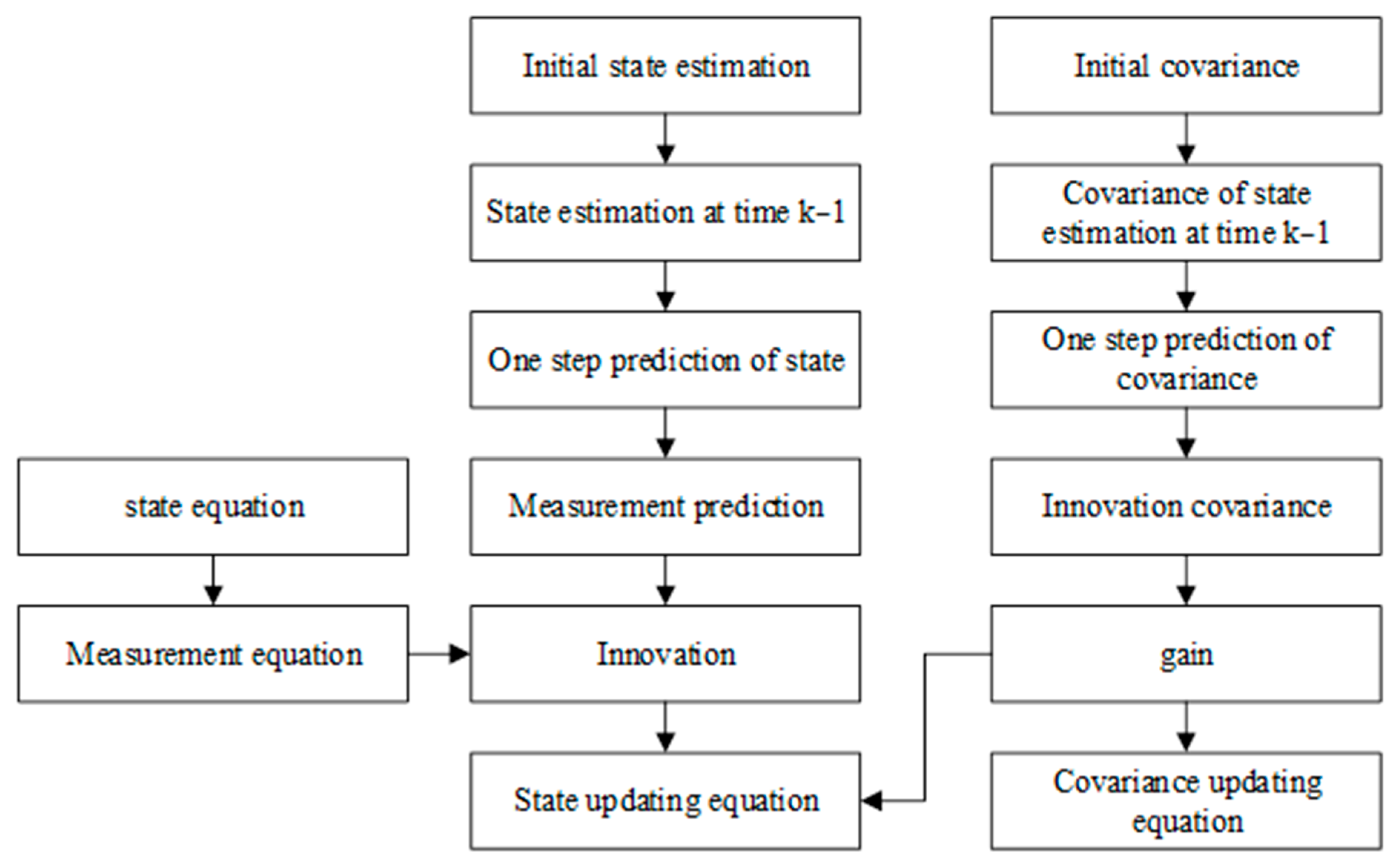
In the update equation, is the correction term of the state prediction value , and also represents the change between the observed extension and the true value in size, shape and direction (geometric distortion caused by the sensor to the target measurement). In this paper, the centroid state of the target can be estimated more accurately by the introduction of , and the use of these innovation concerning the real noise. In addition, Equation (20) incorporates the real measurement noise into the estimation process of , so the information of extended can be estimated more accurately. When the predicted is different from the basic extended definition, this method can be used to improve the estimation results by combining more dynamic prior information, and can be adjusted appropriately to accurately describe different situations. Figure 4 is the single-cycle flow chart of the extended target location and extended information filter algorithm.
If the current time is the first time, initialize N measurement clusters into N expansion targets in sequence. The initial position of the expansion target that corresponds to the in the random matrix based on the tracking of the expansion target is the mean of the measurement clusters. The initial length is 100 m, the initial width is 50 m and the initial orientation is 270°, that is, 23° east by north, corresponding to in the random matrix based on the tracking of the expansion target. If the current time is not the first time, each tracked track is predicted based on the method of random matrices. Then, based on the nearest-neighbor method, the measurement clusters falling into the corresponding wave gate are assigned to the existing tracks and updated based on the random matrices. For the remaining clusters that do not fall into any existing track gate, a new track is initialized again based on random matrices. The data processing flow of the fusion algorithm of extended target tracking for converted measurements is shown in Figure 5.
4. Experimental Section
The measured data are from two different groups of sea surface targets. Dataset 1 is from a fishing boat in the Bohai Sea, with a size of 120 m × 10 m. The boat is positioned about 9 km from the radar’s position. The boat keeps moving straight at a velocity of 10 m/s toward the azimuth of 23° east of north. The radar sampling time is 150 s. Dataset 2 is from sea targets with different sizes, azimuths and velocities in the Bohai Sea. The target group is located about 5 km away from the radar’s position. The group targets do not specify their respective movement status or the course of the ships. The radar sampling time is 300 s.
4.1. Single-Target Tracking
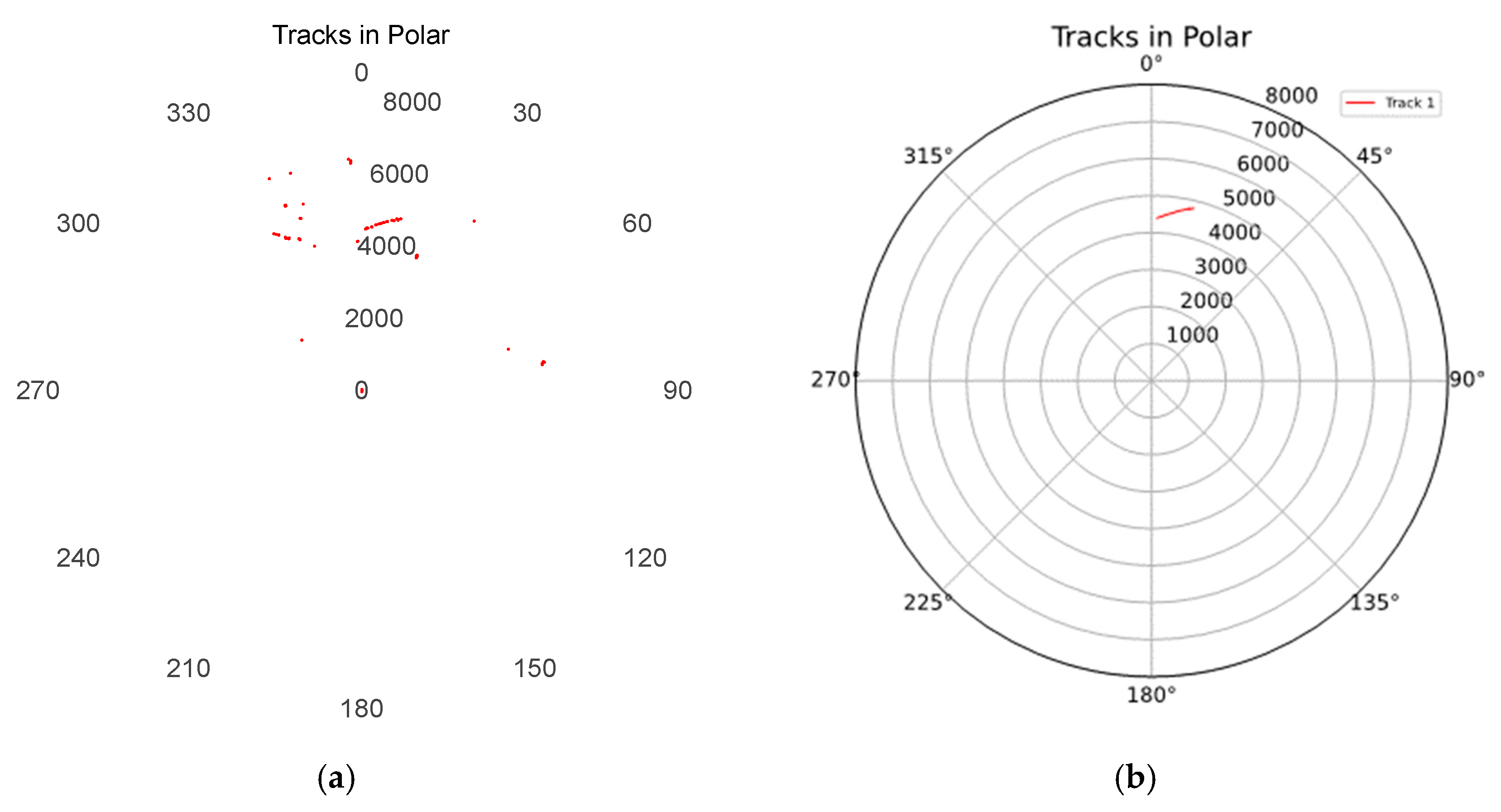
Single-target information of the fishing boat is collected by the radar for testing. The navigation process of the fishing boat is in a state of almost uniform linear motion. In this scenario, the range resolution of the radar is 6.511 m, and the effective detection range is 6 km; 50 frames are used to track the target. The target’s tracks in polar coordinates are shown in Figure 6.
According to the analysis of Figure 6a, many track breakdowns occurred during target tracking, and the sea clutter in the scene has not been completely processed, resulting in false tracks. There are three reasons for this:
- (1)
- The expansion of the targets is not taken into account. Since the length of the target is more than 100 m, the position of the center point after clustering is not guaranteed to be the center of the actual ship, and there will be a deviation.
- (2)
- The normalization error in clustering is relatively large, and it cannot be converted to Cartesian coordinates for tracking. It is difficult to accurately ensure that the ship keeps a constant velocity and conforms to the motion model by using the difference method to calculate the velocity.
- (3)
- The gate setting is too small, and the number of frames selected for track termination is small.
Subsequently, in view of the above problems, the extended target algorithm under a converted measurement Kalman filter (CMKF-REMTT) is used to make the tracking effect more accurate. At the same time, the size, velocity and azimuth of the target model can be deduced according to the measurement return values of the extended targets. The improved track using the extended target tracking is shown in Figure 6b.
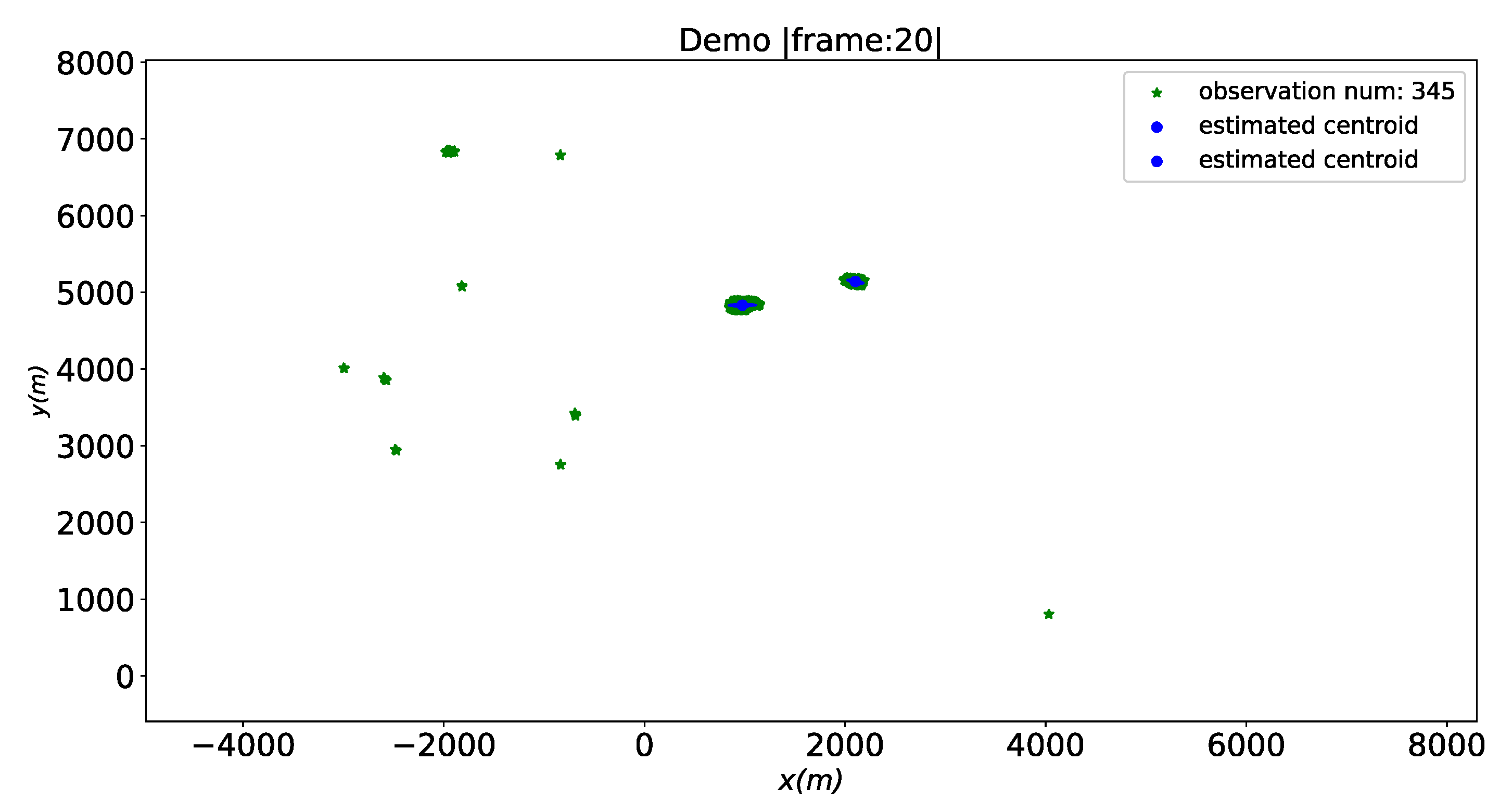
The extended target tracking algorithm based on the converted measurement Kalman filter cannot form a stable two-dimensional model in multiple frames because the clutter points do not have a fixed shape. The method in this paper can better filter the clutter while tracking and solve the problem of correlated clutter while point-target tracking. The tracking performance can be more stable using polar coordinates, and more information can be fed back to facilitate tracking. The target tracking effect is shown in Figure 7, Figure 8, Figure 9, Figure 10 and Figure 11, in which the horizontal and vertical coordinates (0, 0) are ground, and the radar rotates 360 degrees at the current position to obtain the movement information of the fishing boat at sea.
The research results in Figure 8, Figure 9 and Figure 11 show that the single fishing boat target has stable model tracking during navigation, and Figure 7 and Figure 10 show that there may be errors or model distortion during radar measurement. It can be seen from the image of the tracking target that the clutter is presented by a green star shape during the tracking process. The clutter cannot form an elliptical model and cannot exist continuously and regularly across multiple frames. The real goal is to use blue dots to represent the center of the target mass and keep the ellipse moving steadily. When the error is small, the tracking can maintain a good model state, and the clutter is presented in the form of points, so false tracks cannot be generated.
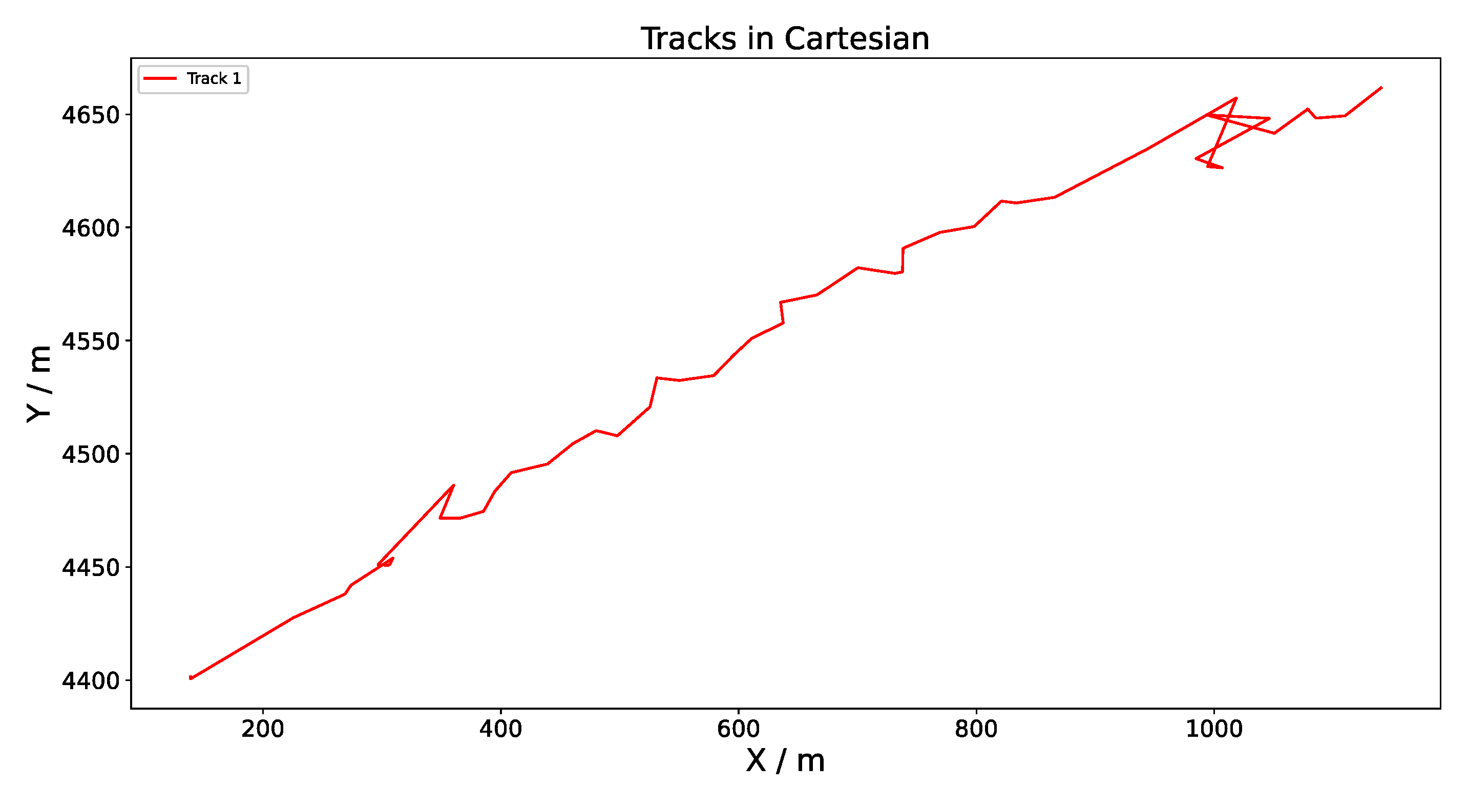
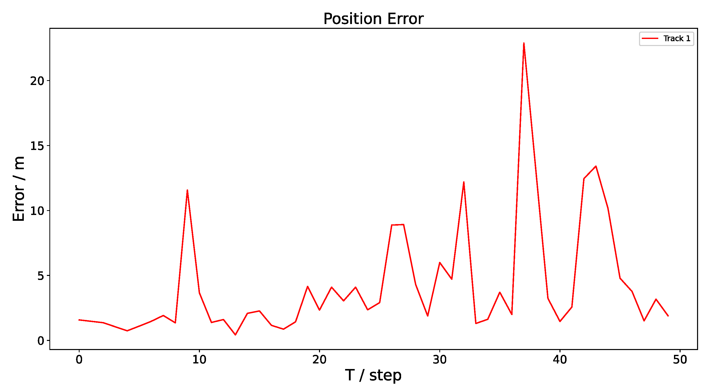
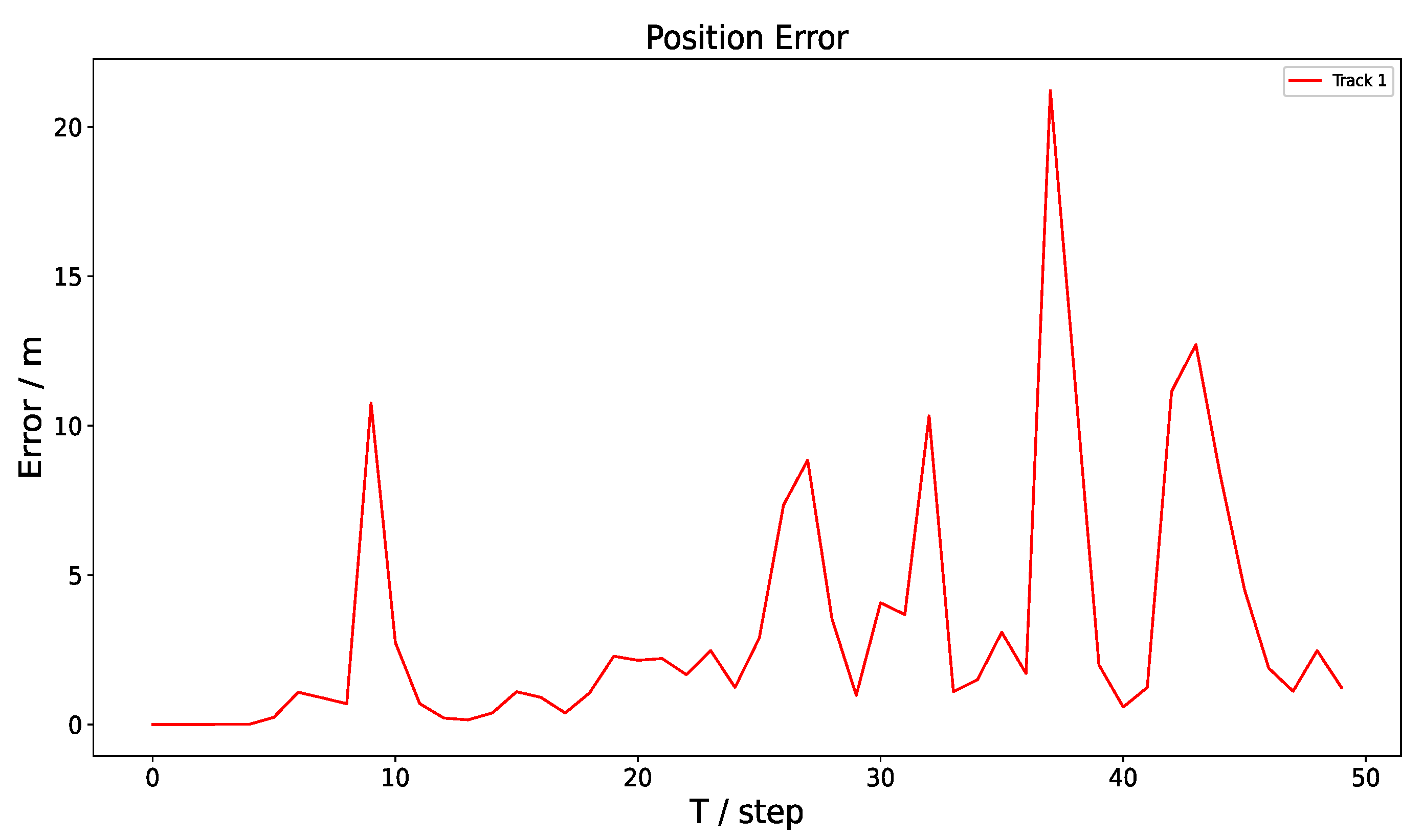
By comparing Figure 12, Figure 13, Figure 14, Figure 15, Figure 16 and Figure 17, it can be seen that using the standard coordinate transformation, the accuracy of the target along the track is lower, the extreme values of distance error and speed are slightly smaller, the stability of the curve is slightly better and the tracking accuracy is improved. From the analysis of Figure 12 and Figure 15, the targets in the Cartesian coordinates keep moving in a straight line, and the error between measurements and tracking stays at about 5 m. Compared with the size of the fishing boat, the short tracking error distance of 5 m can be ignored. Figure 17 and Figure 18 show the velocity and size estimation of the fishing boat in each frame. The following two reasons cause the fluctuation in velocity: (1) The fishing boat does not keep a constant velocity, and the position prediction is inaccurate. (2) When updating, the filter mainly updates the position information. In this experiment, the observability of the position is stronger than the velocity. However, the velocity is basically kept at 10 m/s, which is consistent with the established uniform rectilinear motion model. The reason for the large change in the target size is that the initial value of the fishing boat is set to be 100 m long and 50 m wide, which indirectly indicates that the greater the number of tracking frames, the better the effect of the estimation method. After 10 frames, the length, width and azimuth of the boats remain stable, which is similar to the initially given target information.
4.2. Multi-Target Tracking
The multi-target information collected by the radar is from a group of sailing fishing boats in the Bohai Sea. In this scenario, the range resolution of the radar is 9.766 m, and the effective detection range is 10 km. The target is tracked by 100 frames of measurement. The preprocessing and filtering process are consistent with the single-target tracking in traditional algorithms; DBSCAN and the extended Kalman filter (EKF) are used, followed by the group target probability association algorithm (GPDA) for data association, and the target tracks are updated. The tracking is performed in polar coordinates, as shown in Figure 19:
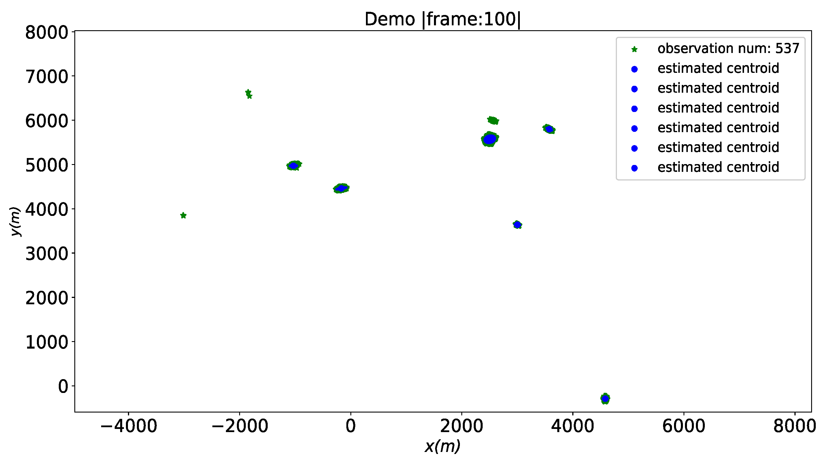
In the comparison in Figure 19, the angle of the navigation radar tacking maps a and b is between 270° and 360°. The traditional point-target tracking algorithm has the problem that the clutter generates false tracks. When tracking multiple targets, the algorithm in this paper not only filters out the points that cannot generate an extended clutter, but also reduces the tracks formed by the measurement targets with 1–2 frames of flicker, which greatly improves the accuracy of target tracking and solves the problem that the multi-target clutter affects the accuracy of track association. The track information of EKF-GPDA and CMKF-RMETT is shown in Table 2, and the results of multi-target tracking are shown in Figure 20, Figure 21, Figure 22, Figure 23 and Figure 24, where the horizontal and vertical coordinates (0, 0) are ground and the radar rotates 360 degrees at the current position to measure the movement information of the fishing boats at sea.
The results in Figure 20, Figure 21 and Figure 22 show that there are not only straight-line fishing boats, but also maneuvering targets and targets with varying velocities in this scene. The estimated number of centroids depends on the ship with the current frame number. Through Figure 15, Figure 16 and Figure 17, the same problem as single-target tracking occurs in that that there may be errors or model distortion during radar measurement. In frame 80, one real target is recognized as multiple tracking targets. In the first 60 frames, the target keeps tracking as three targets, and in the last 40 frames, four targets are added. Because the uniform rectilinear model is adopted for tracking in this paper, there is a situation where one target generates multi-track judgments. The clutter generated in the multi-target tracking still cannot be extended. Subsequently, track deletion is performed for the extended targets with only 1–2 frames, which ensures the tracking of the real moving target only.
By comparing Figure 25, Figure 26, Figure 27, Figure 28, Figure 29 and Figure 30, it is obvious that the stability of the extended target track after measurement conversion is better than that of standard coordinate transformation in multi-target tracking. The tracking distance error and velocity estimation curves are slightly more stable, and the extreme values are also slightly lower. The reason for the large fluctuation in some of the velocity curves is that the Doppler information is not used in the update, the fishing vessel does not move in a uniformly straight-line and the prediction can be biased. According to Figure 28 and Figure 30, it can be seen that the estimation of the tracking error and velocity are in a linear relationship. In the multi-target tracking scenario, studying Figure 26, track 1-3 is my enlarged image of the original seven tracks, the target of track 1 shows no maneuvering in the first 60 frames, shows a stable size and angle during the tracking in the first 70 frames, and has a course deflection in the last 40 frames, which has a great impact on the estimation of the target’s width and angle. The target of track 3 has large variation in its maneuvering. This model has a deviation in angle estimation, and consequently, correct angle estimation cannot be formed. In the multi-target tracking scene, the extended algorithm can still control the error within 3 m, which is negligible compared with the size of large fishing boats and the range resolution of the radar. The research results in Figure 31 also show that the same target breaks in tracks 1 and 3. When the number of measured frames is small, the motion feature information also has large fluctuations and instability.
Table 3 compares three algorithms for point-target tracking, extended target tracking and extended target tracking after measurement conversion in terms of calculation speed, adaptability to the environment and track accuracy.
4.3. Research Findings and Limitations
This paper designed a fusion algorithm (CMKF-RMEOT) for the measurement of target trajectory using sea navigation radar systems. The study optimized the problem of excessive clutter in point-target tracking and more accurately located the precise trajectory of fishing vessels in multi-target tracking. It solved the interference of more sea clutter and also realized the real-time estimation of speed, heading and size of each surface target. In addition, the prediction error is within the range of radar accuracy, which is consistent with the real target motion characteristics. However, in this study, the algorithm needed too many sampling frames to achieve a stable tracking effect, and the sampling interval of 3 s was too long, which also led to a stable result in speed estimation. The same track will be broken and two new tracks will be generated in fishing vessels making larger maneuvers, which will lead to deviation in the tracks from the real situation. The motion of the targets near the sea is complicated because the vessels are prone to greater maneuvering. The motion model of the maneuvering targets can be constructed to achieve more accurate estimation as a further research direction.
5. Conclusions
To solve the problem of the low tracking accuracy of point target under cluttered environment and nonlinear measurement conditions (distance and angle), this paper improved the accuracy of transforming polar coordinates to Cartesian coordinates based on the idea of converted measurement. The extended target tracking algorithm was introduced into the measurement under a high resolution to expand the target and describe the evolution and observation distortion of the object expansion. A fusion-tracking algorithm for obtaining the converted measurement and random matrices expansion (CMKF-REMTT) was used to verify the measured data. The experimental results showed that this method not only reduces computational load and time of the traditional algorithm, but can also track the target accurately in a highly nonlinear environment. The distance error was far less than the threshold of the navigation safety distance, improving the accuracy of the tracking. It suppressed the influence of clutter on the real track, and the tracked target fed back more kinematic characteristics. In the future, a tracking model capable of identifying maneuvering targets will be built to accurately locate the track, and a radar network composed of three radars will be subsequently set up to conduct multi-sensor data fusion on the target, so as to further improve the tracking accuracy.
Author Contributions
Data curation, W.F.; formal analysis, W.F.; methodology, W.F. and H.Z.; software, H.Z.; supervision, F.T.; validation; visualization, H.Z.; writing—original draft, F.T. and H.Z.; writing—review and editing, F.T. All authors have read and agreed to the published version of the manuscript.
Funding
This research received no external funding.
Institutional Review Board Statement
Not applicable.
Informed Consent Statement
Not applicable.
Data Availability Statement
All the experimental data are from the measured experimental data of the fishing vessel surveillance radar project, providing support for the design algorithm. Due to the nature of this research, participants of this study did not agree for their data to be shared publicly, so supporting data is not available.
Conflicts of Interest
The authors declare no conflict of interest.
References
- Katzmann, A.; Taubmann, O.; Ahmad, S.; Mühlberg, A.; Sühling, M.; Groß, H.M. Explaining clinical decision support systems in medical imaging using cycle-consistent activation maximization. Neurocomputing 2021, 458, 141–156. [Google Scholar] [CrossRef]
- Hernangómez, R.; Visentin, T.; Servadei, L.; Khodabakhshandeh, H.; Stańczak, S. Improving Radar Human Activity Classification Using Synthetic Data with Image Transformation. Sensors 2022, 22, 1519. [Google Scholar] [CrossRef] [PubMed]
- Feldmann, M.; Franken, D.; Koch, W. Tracking of Extended Objects and Group Targets Using Random Matrices. IEEE Trans. Signal Process. 2011, 59, 1409–1420. [Google Scholar] [CrossRef]
- Koch, J.W. Bayesian Approach to Extended Object and Cluster Tracking Using Random Matrices. IEEE Trans. Aerosp. Electron. Syst. 2008, 44, 1042–1059. [Google Scholar] [CrossRef]
- Li, X.R.; Jilkov, V.P. Survey of Maneuvering Target Tracking-Part I: Dynamic Models. IEEE Trans. Aerosp. Electron. Syst. 2003, 39, 1333–1364. [Google Scholar]
- Ma, J.B.; Li, Y.H. CFAR algorithm of millimeter wave LFMCW based on VI-CFAR research. J. Microw. 2021, S1, 134–137. [Google Scholar]
- Lan, J.; Li, X. Extended-object or group-target tracking using random matrix with nonlinear measurements. IEEE Trans. Signal Process. 2019, 67, 5130–5142. [Google Scholar] [CrossRef]
- Lerro, D.; Bar-Shalom, Y. Tracking with debiased consistent converted measurements versus EKF. IEEE Trans. Aerosp. Electron. Syst. 1993, 29, 1015–1022. [Google Scholar] [CrossRef]
- Zhao, Z.; Chen, H.; Chen, G.; Kwan, C.; Li, X.R. Comparison of several ballistic target tracking filters. In Proceedings of the 2006 American Control Conference, Minneapolis, MN, USA, 14–16 June 2006; p. 6. [Google Scholar]
- Zhao, Z.; Chen, H.; Chen, G.; Kwan, C.; Li, X.R. IMM-LMMSE filtering algorithm for ballistic target tracking with unknown ballistic coefficient. In Signal and Data Processing of Small Targets 2006; University of New Orleans (United States): New Orleans, LA, USA; Intelligent Automation Inc.: Albany, OR, USA, 2006; p. 6236. [Google Scholar]
- Lei, C.; Kong, L.J.; Li, S.Q.; Yi, W. The multiple model multi-Bernoulli filter based track-before-detect using a likelihood based adaptive birth distribution. Signal Process. 2020, 171, 107501. [Google Scholar]
- Kwan, C.; Budavari, B. A high-performance approach to detecting small targets in long-range low-quality infrared videos. Signal Image Video Process. 2022, 16, 93–101. [Google Scholar] [CrossRef]
- Schubert, E.; Sander, J.; Ester, M.; Kriegel, H.P.; Xu, X. DBSCAN revisited, revisited: Why and how you should (still) use DBSCAN. ACM Trans. Database Syst. 2017, 42, 1–21. [Google Scholar] [CrossRef]
- Baum, M.; Noack, B.; Hanebeck, U.D. Extended Object and Group Tracking with Elliptic Random Hypersurface Models. In Proceedings of the 13th International Conference on Information Fusion, Edinburgh, UK, 26–29 July 2010; pp. 1–8. [Google Scholar]
- Dong, W.; Wang, J.; Song, Z. Mono-pulse radar angle estimation algorithm under low signal-to-noise ratio. J. Phys. Conf. Ser. 2021, 1914, 012042. [Google Scholar] [CrossRef]
- Waxman, M.J.; Drummond, O.E. A Bibliography of Cluster (Group) Tracking. In Proceedings of the SPIE Conference on Signal and Data Processing of Small Targets, Orlando, FL, USA, 25 August 2004; pp. 551–560. [Google Scholar]
- Guo, Y.; Li, Y.; Tharmarasa, R.; Kirubarajan, T.; Efe, M.; Sarikaya, B. GP–PDA filter for extended target tracking with measurement origin uncertainty. IEEE Trans.-Actions Aerosp. Electron. Syst. 2019, 55, 1725–1742. [Google Scholar] [CrossRef]
- Ehrman, L.M.; Lanterman, A. Extended Kalman filter for estimating aircraft orientation from velocity measurements. Radar Sonar Navig. IET 2018, 2, 12–16. [Google Scholar] [CrossRef]
- Granstrom, K.; Orguner, O. New prediction for extended targets with random matrices. IEEE Trans. Aerosp. Electron. Syst. 2014, 50, 1577–1589. [Google Scholar] [CrossRef] [Green Version]
- Sun, L.; Zhang, J.; Yu, H.; Fu, Z.; He, Z. Maneuvering Extended Object Tracking with Modified Star-Convex Random Hypersurface Model Based on Minimum Cosine Distance. Remote Sens. 2022, 14, 4376. [Google Scholar] [CrossRef]
- Liu, S.; Liang, Y.; Xu, L. Maneuvering extended object tracking based on constrained expectation maximization. Signal Process. 2022, 201, 108729. [Google Scholar] [CrossRef]
- Liu, J.; Wang, Z.; Cheng, D.; Chen, W.; Chen, C. Marine Extended Target Tracking for Scanning Radar Data Using Correlation Filter and Bayes Filter Jointly. Remote Sens. 2022, 14, 5937. [Google Scholar] [CrossRef]
- Guo, Y.; Yang, D.; Ren, L.; Yan, L. Gaussian processes based extended target tracking in polar coordinates with input uncertainty. EURASIP J. Adv. Signal Process. 2022, 2022, 106. [Google Scholar] [CrossRef]
- Zhang, X.; Yan, Z.; Chen, Y.; Yuan, Y. A novel particle filter for extended target tracking with random hypersurface model. Appl. Math. Comput. 2022, 425, 127081. [Google Scholar] [CrossRef]
- Wang, S.; Bao, Q. Decorrelated unbiased converted measurement for bistatic radar tracking. J. Appl. Remote Sens. 2021, 15, 016507. [Google Scholar] [CrossRef]
- Wang, G.; Feng, X. Unbiased converted measurement manoeuvering target tracking under maximum correntropy criterion. Cogn. Comput. Syst. 2020, 2, 125–129. [Google Scholar] [CrossRef]
- Bordonaro, S.; Willett, P.; Barshalom, Y. Decorrelated unbiased converted measurement Kalman filter. IEEE Trans. Aerosp. Electron. Syst. 2014, 50, 1431–1444. [Google Scholar] [CrossRef]
- Liu, S.; Li, H.; Zhang, Y.; Zou, B. Multiple hypothesis method for tracking move-stop-move target. J. Eng. 2019, 2019, 6155–6159. [Google Scholar] [CrossRef]
Figure 1.
Measured sea area and radar in Bohai Sea.

Figure 2.
PPI information of vessel navigation (single targets).

Figure 3.
PPI information of vessel navigation (multiple targets).

Figure 4.
Block diagram of the REMTT filter algorithm.

Figure 5.
Flow chart of the CMKF-REMTT fusion algorithm.

Figure 6.
Polar coordinate tracking under single-target tracking. (a) The point target’s tracks. (b) The extended targets’ tracks.
Figure 6.
Polar coordinate tracking under single-target tracking. (a) The point target’s tracks. (b) The extended targets’ tracks.

Figure 7.
Single target in the Cartesian coordinate system tracking in the 10th frame.

Figure 8.
Single target in the Cartesian coordinate system tracking in the 20th frame.

Figure 9.
Single target in the Cartesian coordinate system tracking in the 30th frame.

Figure 10.
Single target in the Cartesian coordinate system tracking in the 40th frame.

Figure 11.
Single target in the Cartesian coordinate system tracking in the 50th frame.

Figure 12.
Single-target track in the Cartesian coordinate system (REMTT).

Figure 13.
Single-target track in the Cartesian coordinate system (CMKF-REMTT).

Figure 14.
Tracking error between the prediction and actual track (REMTT).

Figure 15.
Tracking error between prediction and actual track (CMKF-REMTT).

Figure 16.
Tracking error between the prediction and actual track (REMTT).

Figure 17.
Single-target velocity estimation (CMKF-REMTT).

Figure 18.
Estimation of the single target’s size and azimuth.

Figure 19.
Tracks in polar coordinates under multi-target tracking. (a) Tracks of point-target tracking. (b) Tracks of extended target tracking.
Figure 19.
Tracks in polar coordinates under multi-target tracking. (a) Tracks of point-target tracking. (b) Tracks of extended target tracking.

Figure 20.
Multi-target tracking in the Cartesian coordinate system in the 20th frame.

Figure 21.
Multi-target tracking in the Cartesian coordinate system in the 40th frame.

Figure 22.
Multi-target in the Cartesian coordinate system tracking in the 60th frame.

Figure 23.
Multi-target tracking in the Cartesian coordinate system in the 80th frame.

Figure 24.
Multi-target tracking in the Cartesian coordinate system in the 100th frame.

Figure 25.
Multi-target tracking in the Cartesian coordinate system (REMTT).

Figure 26.
Multi-target tracking in the Cartesian coordinate system (CMKF-REMTT).

Figure 27.
Tracking error between the prediction and actual track (REMTT).

Figure 28.
Tracking error between the prediction and actual track (CMKF-REMTT).

Figure 29.
Multi-target velocity estimation (REMTT).

Figure 30.
Multi-target velocity estimation (CMKF-REMTT).

Figure 31.
Estimation of the multi-target size and azimuth.


Table 1.
Partial parameters and performance indices of sea surface navigation radar.
| System Parameters and Performance Index of Radar | Parameter |
|---|---|
| Sampling period (s) | 3 |
| Effective detection range (km) | adjustable |
| Velocity detection range (m/s) | −50~50 |
| Range resolution (m) | adjustable |
| Angle resolution (°) | 0.17 |
Table 2.
Comparison of tracking results under point target and extended target tracking methods.
| EKF-GPDA | CMKF-RMEOT | |
|---|---|---|
| Number of clusters | 11 | 12 |
| Number of generated tracks | 15 | 7 |
| Number of correct tracks | 6 | 6 |
| Tracking accuracy | 40% | 85.8% |
Table 3.
Comprehensive comparison of three algorithms.
| Algorithm | Calculation Speed | Maximum Tracking Distance Error | Tracking Accuracy | Adapt to the Environment | Linearity |
|---|---|---|---|---|---|
| EKF-GPDA | 8.5 s | 10 m | 40% | white Gaussian noise | weak nonlinearity |
| REMTT | 1.8 s | 4.5 m | 85.8% | white Gaussian noise | linear |
| CMKF-REMTT | 2.1 s | 3 m | 85.8% | white Gaussian noise | unlimited |
Disclaimer/Publisher’s Note: The statements, opinions and data contained in all publications are solely those of the individual author(s) and contributor(s) and not of MDPI and/or the editor(s). MDPI and/or the editor(s) disclaim responsibility for any injury to people or property resulting from any ideas, methods, instructions or products referred to in the content. |
© 2023 by the authors. Licensee MDPI, Basel, Switzerland. This article is an open access article distributed under the terms and conditions of the Creative Commons Attribution (CC BY) license (https://creativecommons.org/licenses/by/4.0/).
Share and Cite
MDPI and ACS Style
Tian, F.; Zhang, H.; Fu, W. Research on Extended Target-Tracking Algorithms of Sea Surface Navigation Radar. Electronics 2023, 12, 616. https://doi.org/10.3390/electronics12030616
AMA Style
Tian F, Zhang H, Fu W. Research on Extended Target-Tracking Algorithms of Sea Surface Navigation Radar. Electronics. 2023; 12(3):616. https://doi.org/10.3390/electronics12030616
Chicago/Turabian StyleTian, Feng, Haoyu Zhang, and Weibo Fu. 2023. "Research on Extended Target-Tracking Algorithms of Sea Surface Navigation Radar" Electronics 12, no. 3: 616. https://doi.org/10.3390/electronics12030616
Note that from the first issue of 2016, this journal uses article numbers instead of page numbers. See further details here.