Article

Prediction of Critical Filling of a Storage Area Network by Machine Learning Methods

by
Igor S. Masich
,
Vadim S. Tynchenko
*,
Vladimir A. Nelyub
,
Vladimir V. Bukhtoyarov
,
Sergei O. Kurashkin
*,
Andrei P. Gantimurov
and
Aleksey S. Borodulin
Artificial Intelligence Technology Scientific and Education Center, Bauman Moscow State Technical University, 105005 Moscow, Russia
*
Authors to whom correspondence should be addressed.
Electronics 2022, 11(24), 4150; https://doi.org/10.3390/electronics11244150
Submission received: 2 November 2022 / Revised: 6 December 2022 / Accepted: 8 December 2022 / Published: 12 December 2022

Abstract

:
The introduction of digital technologies into the activities of companies is based on software and hardware systems, which must function reliably and without interruption. The forecasting of the completion of storage area networks (SAN) is an essential tool for ensuring the smooth operation of such systems. The aim of this study is to develop a system of the modelling and simulation of the further loading of SAN on previously observed load measurements. The system is based on machine learning applied to the load prediction problem. Its novelty relates to the method used for forming input attributes to solve the machine learning problem. The proposed method is based on the aggregation of data on observed loading measurements and the formalization of the problem in the form of a regression analysis problem. The artificial dataset, synthesized stochastically according to the given parameter intervals and simulating SAN behavior, allowed for more extensive experimentation. The most effective algorithm is CatBoost (gradient boosting on decision trees), which surpasses other regression analysis algorithms in terms of R2 scores and MAE. The selection of the most significant features allows for the simplification of the prediction model with virtually no loss of accuracy, thereby reducing the number of confessions used. The experiments show that the proposed prediction model is adequate to the situation under consideration and allows for the prediction of the SAN load for the planning period under review with an R2 value greater than 0.9. The model has been validated on a series of real data on SAN.

1. Introduction

Storage area networks (SAN) constitute a software and hardware complex for organizing the reliable storage of various types of data and providing quick and guaranteed access to them. SAN are an essential component of information systems for organizations that process large volumes of data and use them to implement decision support systems. Each storage area network has a number of characteristics that affect its performance in a particular organization. One of the important characteristics is the size of the used volumes (memory capacity), which affects the cost of purchased and installed equipment. An organization implementing SAN in its information structure may not be able to install volumes large enough to suffice for long periods. In this case, to organize uninterrupted system functioning, it is necessary to know when volume filling of the system will be critical to the ability to complement the storage system with additional resources in advance. Thus, from a practical point of view, the task of predicting the filling or loading of SAN is very relevant.
In this work, the input data are observations (measurements) of the filling of the SAN, which contain the date and time, as well as the value of the degree of filling at a point in time. The task of predicting the loading of the SAN can be formulated in two ways: as a “Direct” question: what will the occupancy be at a given time interval in the future? Alternatively, the task can be approached from a practical point of view, wherein it is also interesting to answer the “dual” question: at what time will the SAN load reach a certain critical value?
This problem could be considered simply as a time series prediction problem. However, in the general case, the situation under consideration is of a more complex nature. The data series contains sections of loading, including growth, periods of idle time, and the short-term decline of loading. There are also areas of steep decreases in loading that appear due to memory clearing. This paper proposes that the entire time series of data be broken down into loading plots that form a subsample of the data. These sections can be viewed as complex observations from which the training and test datasets are composed. Each complex observation, in turn, represents a time series of data in which there is no volume cleaning procedure. The complex observations (segments) themselves have no order between them. Such a formulation of the problem does not correlate with the usual problem of time series prediction. In this paper, this problem is considered as a problem of regression analysis, in which it is necessary to predict the value of loading after a certain time interval (after a certain number of measurements). However, using solely loading values in past measurements (within the given loading phase) as input data sometimes leads to unsatisfactory results. To generate a predictive model, it is proposed to use the calculated indicators, considering the “velocity” of load growth and the “acceleration” of growth as input data. The effectiveness of the approach is confirmed by the results of the analysis of both real and specially generated synthetic data.
The load prediction problem is relevant for different areas, including energy systems [1]. So, the problem of load forecasting for power systems using a Bayesian approach is considered in [2].

2. Related Works

To solve such problems, we can observe the application of machine learning and data-mining methods. In addition, there are related problems in which the tasks of predicting the performance of servers and central processors are solved.
Server stability depends on various performance metrics, such as the processing capacity, random-access memory (RAM), storage, the network adapter’s characteristics (network operability), and network services. The AIOPS—Artificial Intelligence for IT Operations—approach is proposed in [3]. It is an approach that uses artificial intelligence to manage IT infrastructure based on a layered platform that automates data processing and decision making using machine learning and big data analytics stemming from various elements of the IT infrastructure in real time. AIOPS includes data collection, modeling, and forecasting processes. The paper proposes using an AIOPS-based platform to predict alerts for server stability. The platform includes data collection and preprocessing, time series modeling using ARIMA, and alert prediction. Central processing unit (CPU) utilization is considered as an indicator of server stability.
In the context of the growing importance of cloud-based IT solutions, companies are looking to increase flexibility and reduce costs. The workload in the form of CPU utilization often fluctuates. In [4], the prediction of future CPU workload using the Long Short-Term Memory Networks (LSTM) model is discussed. By predicting future workload, companies can accurately scale their capacity and avoid unnecessary costs and environmental damage. LSTM are compared to recurrent neural networks (RNN). Loads are predicted one step ahead and 30 min into the future. The results show that this approach can be a useful tool for business applications hosted in the public cloud.
Resource demand forecasting allows public cloud service providers to actively allocate or release resources for cloud services. In [5], the prediction of CPU utilization, both in the short and long terms, is discussed. To conceive of the model characteristics that are best-suited for specific types of prediction tasks, two different approaches are considered: the SARIMA time series prediction model as well as a neural network, namely, the LSTM model. These models are applied to data with a lag of 20 min in order to predict usage over the next hour for a short-term task and over the next three days for a long-term task. The SARIMA model outperformed the LSTM in the long-term prediction task but performed worse in the short-term task. In addition, the LSTM model was more robust, while SARIMA was superior in terms of data with a strong seasonal component.
In [6,7], which were devoted to load forecasting using artificial intelligence and machine learning, the authors propose the use of seasonal-trend decomposition using a LOESS (STL)—Local regressions—Local polynomial regressions method. STL allows one to study the distribution and degradation of memory, as well as analyze the comparison with the sample, as a result of which periodic changes in the configuration in the metric will be automatically corrected. Prediction requires algorithms that can analyze SAN load patterns and detect anomalies in daily usage trends.
Besides prediction, ML can also be used to improve anomaly detection. Here, adaptive thresholds for various indicators are set using ML and analyzing historical data, detecting anomalies and triggering appropriate alerts.
In [8,9], the researchers focused on collecting system resource data to predict usage levels in the near future so that the operating system could balance system resources. These studies showed that using data collected in fractions of a second accurately predicted the next step, but could not easily predict resource usage several steps ahead. The results of these attempts showed that the magnitude of the error increased with the number of steps and that the predictions were less effective. The researchers took the results of the short-term predictions and extended them to plan requests in web services. However, this study also showed that when planning was extended several steps into the future, the error rate was unacceptable. The levels of network usage were combined into ninety-minute cycles to reduce the fluctuations observed at shorter times. This study used simple moving averages (SMA), exponential moving averages (EMA), and cubic spline (CS) forecasts to examine the effectiveness of providing long-term forecasting. By creating aggregated data with coarser granularity, the predictability of the range of resource usage based on the seasonality of hours, days, and weeks was studied. The resources evaluated were CPU utilization, free memory, outbound/inbound network traffic, disk-writing time, and disk-reading time. The aggregated data were processed using SMA or EMA to generate a prediction and a confidence interval that matched the administrator’s needs. The actual data set was then compared to the prediction and confidence interval to determine whether the resource was still operating normally, and then the next prediction was generated for the next cycle.
Unpredictable user behavior causes variability in server workload distribution. This topic is addressed in [10,11], where server performance metrics are characterized and modeled using a fuzzy approach. A fuzzy inference system is generated using web server performance metrics and a server utilization index is derived to determine server utilization states for each time period. A fuzzy Markov mode is proposed to illustrate transitions of server resource utilization states based on experts’ linguistic estimation of the probability of a stationary transition. The steady-state algorithm is used to study the convergence of server resource utilization after a certain number of transition periods.
A semi-supervised learning approach can be used to predict extreme CPU utilization [12]. Semi-supervised learning for classification tasks is used in the cited paper to investigate a model for predicting an unpredictable load on IT systems and predicting extreme CPU utilization in a complex corporate environment with many applications running simultaneously. This proposed model predicts the probability of a scenario in which an extreme load affects IT systems, and this model predicts CPU utilization under extreme load conditions. An enterprise IT environment consists of many applications running in a real-time system. The characteristics of the workload patterns are hidden in the transactional data of the applications. This method simulates and generates synthetic server load patterns, runs the scenarios in a test environment, and uses the model to predict excessive CPU utilization under peak load conditions for validation. The expectation maximization classifier with forced learning attempts to extract and analyze parameters that can maximize the model’s chances after removing unknown labels. As a result of this model, the probability of excessive CPU utilization can be predicted in a short period of time compared to several days in a complex enterprise environment.
The authors of [13] propose a methodology for differentiated data storage capacity building based on a predictive model of time series incorporating an estimation of the volume of incoming traffic for storage. The influence of the structure of the incoming data flow on the choice of the prediction model is considered. The state of the SAN is represented in the form of patterns. The patterns are constructed using systematic slices of SAN load values. A periodic analysis of the patterns of the data storage state enables an estimation of the time to reach the limit value of the storage capacity. The predictive model underlying the methodology of the differentiated data storage capacity build-up considers the structure of the incoming data stream. If the incoming traffic possesses a self-similar structure, the predictive model of autoregressive and pro-integrated moving averages is implemented. For traffic without a self-similar structure, a general linear time series prediction model with known past values is implemented. The peculiarities of the structure of the stored traffic are given. The self-similarity properties are verified using LTE traffic as an example, demonstrating the presence of distributions with “heavy tails”. Using the autoregression model and the integrated moving average, the results of predicting the volume of incoming traffic for storage were obtained. The methodology of increasing data storage capacity considers the structure of the incoming data stream, allows for the organization of differentiated increases in storage capacity according to the characteristics of files, and ensures the requirements of guaranteed storage times.
In [14], the structure of a hardware–software complex of physical data storage management for systems that can be used by the owners of technological communication networks to store traffic is proposed. Management mechanisms are considered, such as the distribution of data across different carriers using Kohonen neural networks and the prediction of increases in storage capacity by means of a statistical model and machine learning methods.
In [15], an SAN utilization prediction model was proposed for the timely scaling of storage infrastructure based on predictive estimates of the moment when the storage medium reaches maximum capacity. An SAN capacity management model was developed based on the analysis of storage system state patterns. In the study, the representative pattern is a matrix in which each cell reflects the state of the storage medium’s occupancy at the corresponding level in the storage system’s hierarchical structure. Solving the scaling problem for a storage area network entails predicting the moments when the storage capacity limit and maximum storage capacity are reached. The difference between the predicted estimates is the time available to the administrator for connecting additional media. The research proposes the prediction of SAN utilization values by machine learning methods, namely, Decision trees, Random Forest, Feedforward neural networks, and SVM. It is shown that machine learning methods are less accurate than ARIMA in making short-term forecasts. However, for long-term forecasts, machine learning methods give results comparable to ARIMA results. The proposed SAN load prediction model automates the process of media connectivity, which helps to prevent the loss of data entering the system.
According to the relevant publications, tasks of this type are relevant. Some works estimate the volume of incoming data in storage systems based on the structure of the incoming data flow and on the loading patterns, which is unrealizable for the problem considered here since such information is missing.
However, of particular interest are the findings that the ARIMA method has an advantage only when making short-term forecasts. Machine-learning methods have more advantages when making some long-term forecasts. These conclusions are also confirmed by our studies on the comparative efficiency of different models.
There are also works on central processing unit load prediction [16], server load prediction [17], and cloud data centers [18,19] based on machine learning methods, including the use of artificial neural networks of various types [20] and fuzzy logic methods. However, these tasks, although similar, are different from the SAN load prediction problem solved herein.
Our experiments show that there are more efficient approaches besides neural networks. The approach we use is based on the application of machine learning methods to the regression problem on a transformed dataset consisting of integrated features of the loading history.

3. Materials and Methods

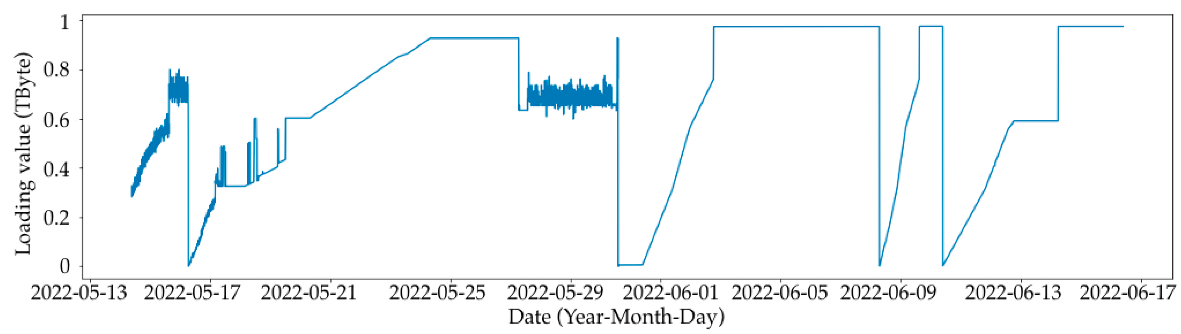
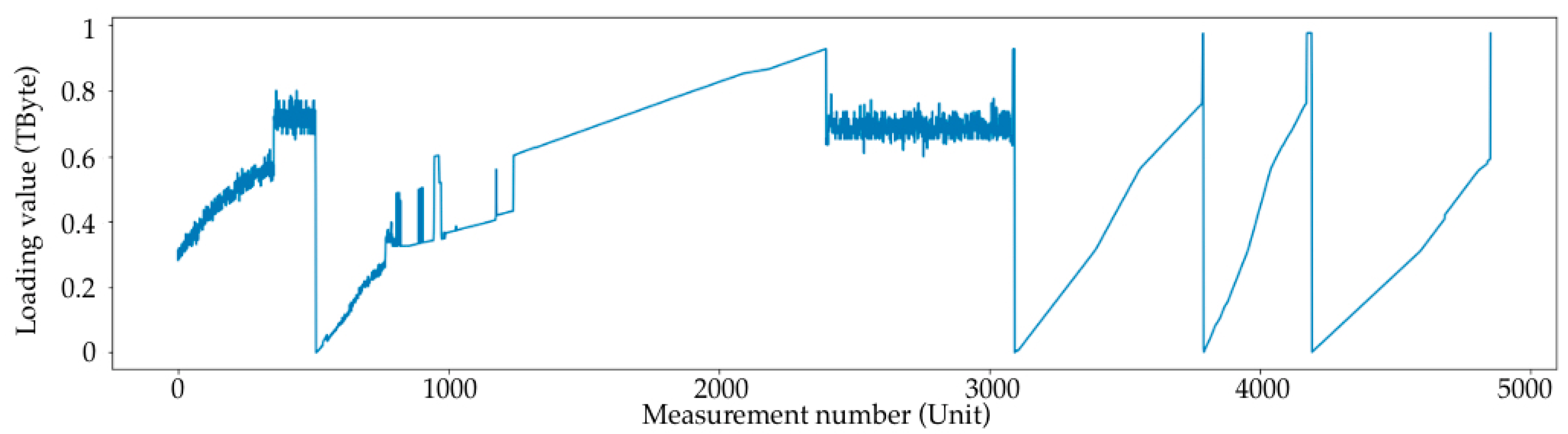
3.1. SAN Loading Simulation

The main task is to develop an algorithm that allows one to predict SAN load (volume), which can then be used in an organization’s information system.
The initial data are SAN fill observations which contain the date, time, and fill values at a given point in time. An example of the raw data (without preprocessing) is shown in Figure 1.
A typical SAN workload graph contains distinct periods of workload growth, periods of idle time, and periods of sharp decrease in workload. Due to the peculiarities of the practical applications of the proposed algorithm, it was decided to simulate only those parts of the dataset that contain periods of load growth. SAN downtimes, or periods in which there is no growth or decline in SAN workload, have been removed from the dataset. In addition, since it is the critical load growth that needs to be predicted, it is important to model only the periods of SAN load growth; accordingly, periods of decreasing load have been removed.
Initially, to select the best model, the target variable, which is the difference between data growth and the volume (the difference between the current value and the value for the previous period), was used. Then, based on the preliminary data estimation, the average period of a storage area network’s full load time is determined. The average period is equated to the planning horizon; in other words, it is the time period in which the full-load prediction of the SAN should be made.
After determining the best model, a prediction is made for the nearest future average period of the full utilization time of the SAN.
Based on the small number of data and large periods without SAN load, the most appropriate approach to this problem is the use of a regression model to predict the target variable Diff (the difference between the current and previous values of the SAN volume load) and exactly predict the load areas from the time when it is already known that the load has started.
The load prediction task can be divided into two stages:
  • A binary classification task: it is necessary to predict whether there will be a significant increase in the volume of data at a future point in time.
  • A regression task. If the forecast of task 1 will be positive, and thus there will be an increase in data, then it is necessary to forecast this volume (target variable). Otherwise, if there is no growth or it is insignificant (for example, in the normal operation of the system), the regression task will not be solved.
  • To solve the regression problem, we pre-processed the data in two variants.
  • The basic variant:
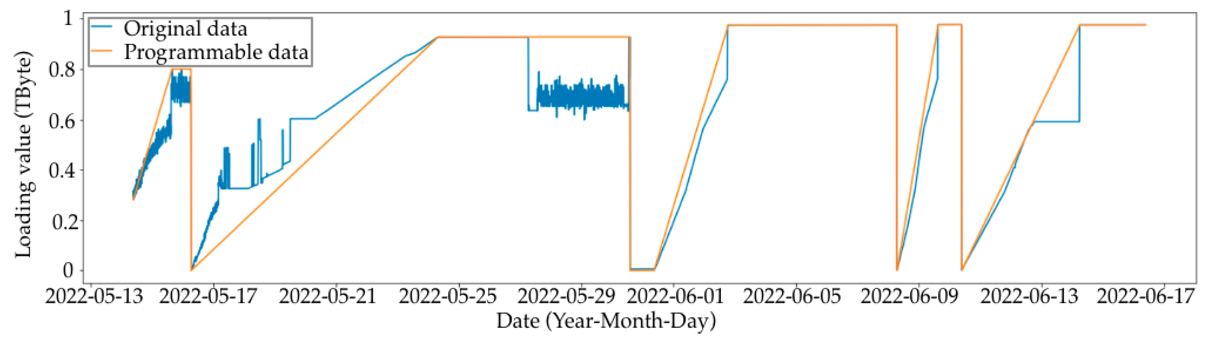
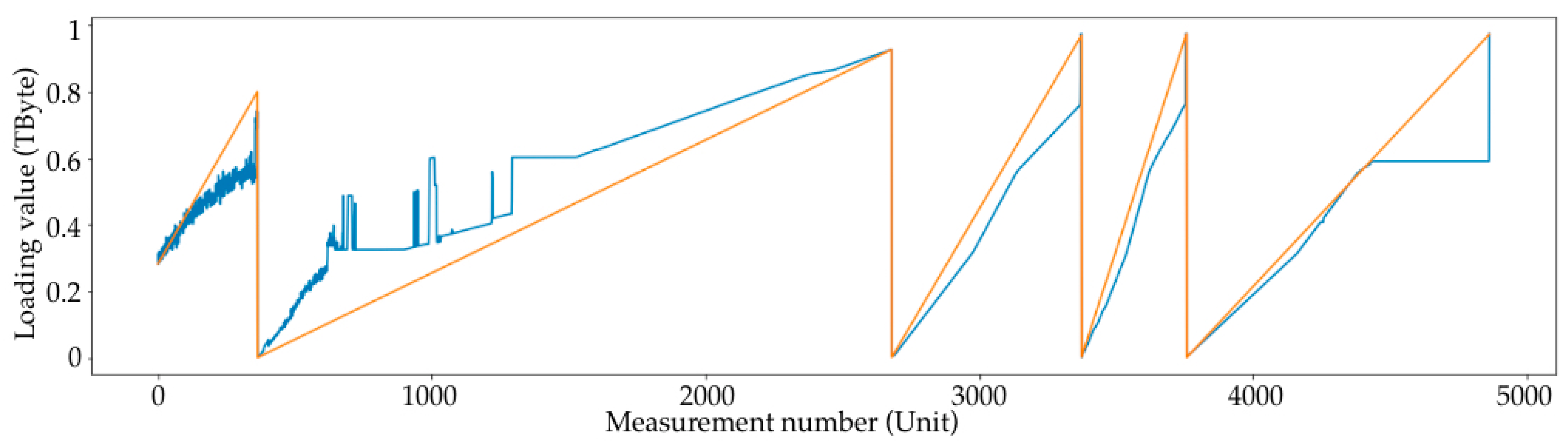
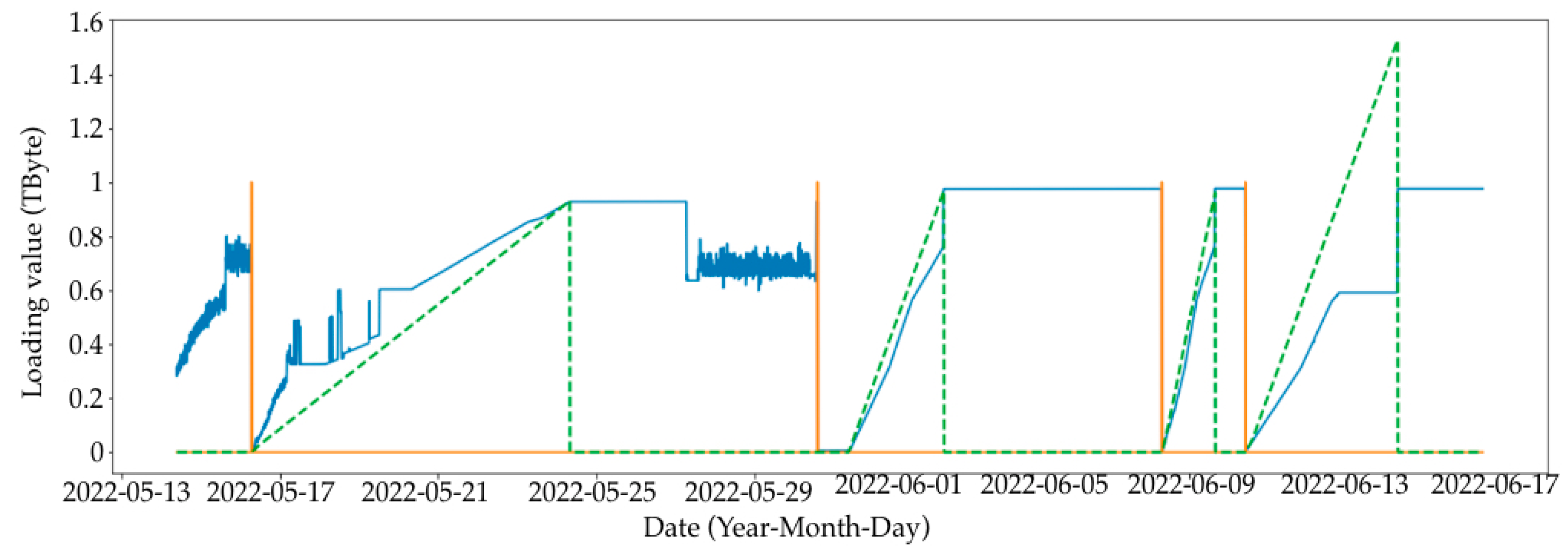
  • Removing periods where there is no load, since there is no way to predict the time when the load will start from a small number of data (Figure 2);
  • Calculating the Diff variable (Figure 3) and deleting sections that have large data deletions to convert the data into a single linear section (Figure 4).
  • Addition to the basic variant:
  • Converting the loading sections to fully linear sections by connecting the beginning and the end of the loading period (Figure 5 and Figure 6) using the averaged Diff value.
Figure 2. Dataset without “downtime” loading, where the measurement numbers are measured sequentially at a certain interval.
Electronics 11 04150 g002
Figure 3. Diff field without areas with large data clearing, wherein measurement numbers are measured sequentially at a certain interval.
Electronics 11 04150 g003
The following graph (Figure 4) visualizes the pre-processed dataset by the Value variable. It was further used to better visualize the estimation of the model’s quality. The information in the graph was obtained by aggregating the variable Diff with the cumulative total.
Figure 4. Value variable. The total linear section of the load, where measurement number is measured sequentially at a certain interval.
Electronics 11 04150 g004
  • Thus, the following actions with the original dataset were performed:
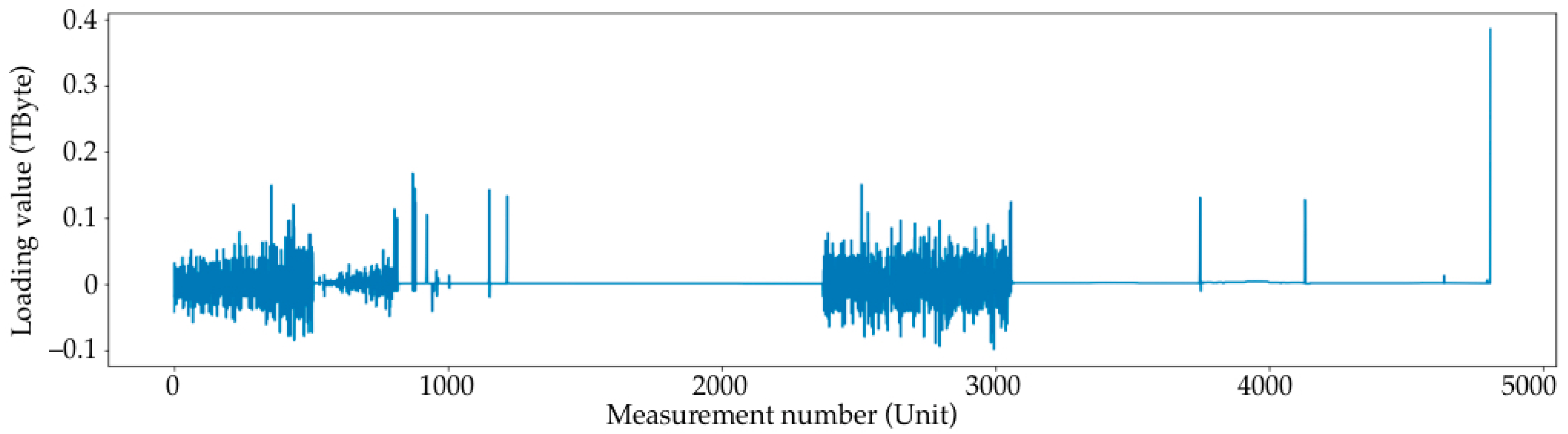
  • The variable “Deviation” (diff) was added, which is the difference between the current SAN load value and the previous one;
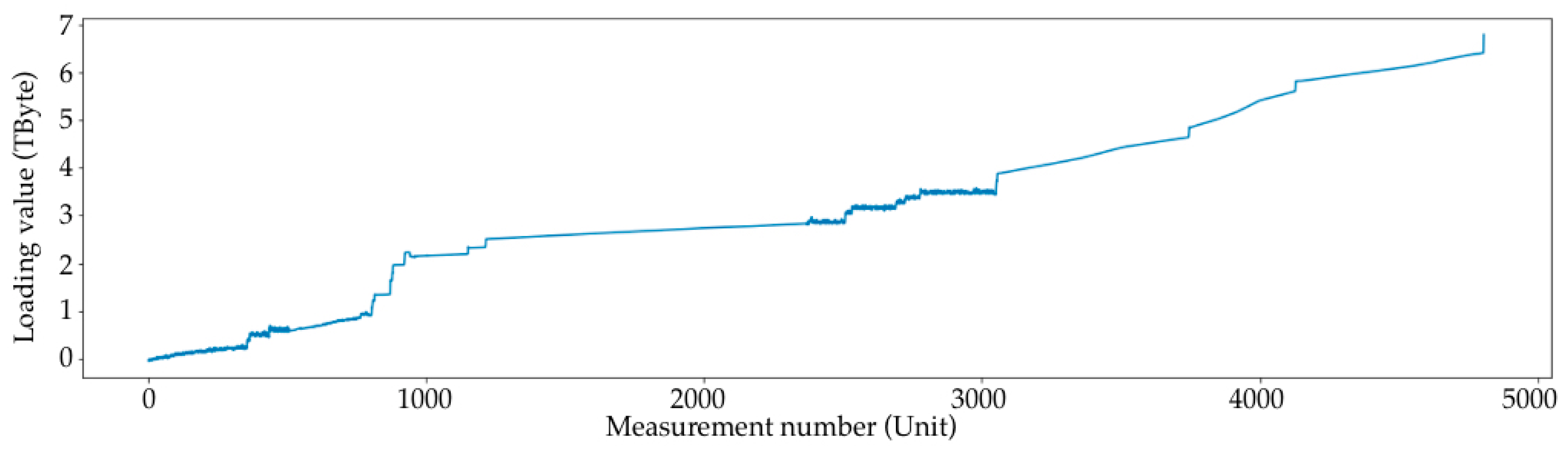
  • SAN downtimes were removed;
  • All the sudden SAN load downturns (more than 10%) were removed, since only the SAN load growth prediction was consistent;
  • The data were smoothed using a moving average (MA) with a period of 50.
As an additional variant of preprocessing, the dataset was converted into linear sections based on the minimum and maximum points of the SAN load value. This approach will hereinafter be referred to as “Smooth Trend”. The result of “Smooth Trend” preprocessing is shown in the graph below (Figure 5 and Figure 6), where the blue line denotes the original “Deviation” data, and the orange line denotes the “Deviation” after preprocessing.
Figure 5. Load plots converted to fully linear sections.
Electronics 11 04150 g005
Figure 6. Linear sections + removed “downtime” loading, where measurement number is measured sequentially at a certain interval.
Electronics 11 04150 g006
Figure 7 shows the forecasts generated by the model. The target variable in this forecast is the variable Diff for one future period (not averaged, and exactly one record ahead). Once the predictions were obtained for all data, they were aggregated with cumulative totals to better visualize the error.
Figure 7. Forecast for 1 future period with subsequent aggregation to cumulative total, where measurement number is measured sequentially at a certain interval.
Electronics 11 04150 g007
Figure 8 visualizes the prediction of each full loading step. For the prediction, 50 previous observations were taken; then, 1 loading step was calculated, and the grid of 50 observations was shifted +1, including 49 real values and 1 predicted value and so on until the end of the loading step (after predicting the 50th step, the model used only predicted values as inputs). The prediction was performed for the period of the real loading step in order to compare the difference between the real value and the predicted value. This graph shows what the prediction error can be depending on the period range.
Figure 8. Forecast for 1 period forward with subsequent aggregation to cumulative total, where measurement number is measured sequentially at a certain interval.
Electronics 11 04150 g008
  • Here, we define the following notation:
  • Diff—the difference between the current value and the previous value;
  • MA—moving average;
  • Lag—number of observations preceding the current one;
  • Shift—shift from the beginning of the loading trend.
  • Table 1 compares the results of SAN utilization prediction according to quality criteria.
Table 1. Comparison of forecasting results.
ModelScore DiffMAPE DiffMAPE ValueRMSE DiffRMSE Value
NN_(162,512)_MA(50)_Diff
Lag_50_Shift_50
0.91641312.590.310.0334010.950863
NN_(162,512)_MA(50)_Diff
Lag_50_Shift_50_Even_trend
0.8589940.190.060.0127020.288143
CatBoost_MA(50)_Diff_Shift_500.57387112.480.160.0736460.480208
CatBoost_MA(50)_Diff
Lag_50_Shift_50
0.57387112.480.160.0736460.480208
KNN_MA(50)_Diff
Lag_50_Even_trend
0.9533490.040.000.0061420.084444
KNN_MA(50)_Diff
Lag_50_Shift_50_Even_trend
0.9533490.040.000.0061420.084444
List of the models used:
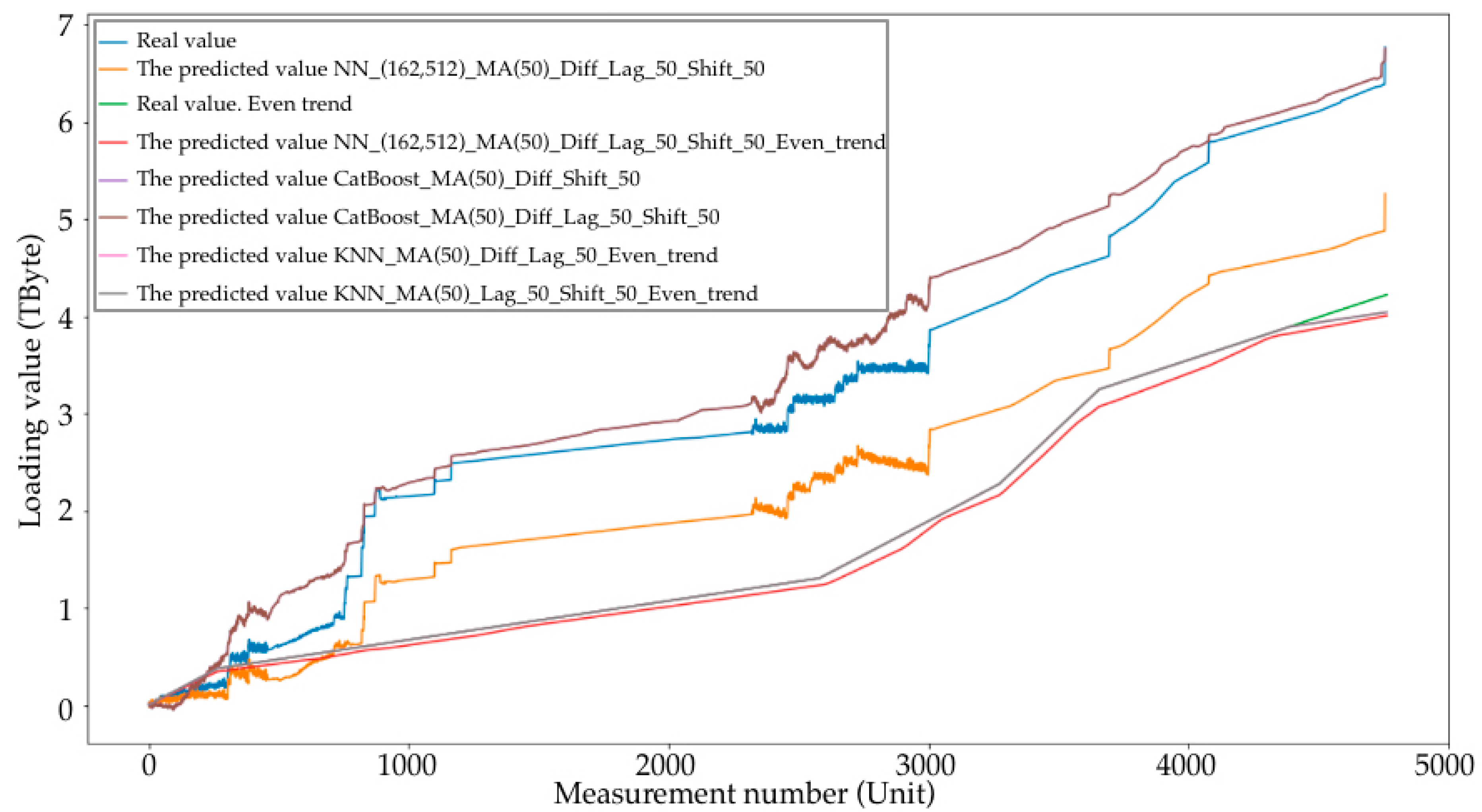
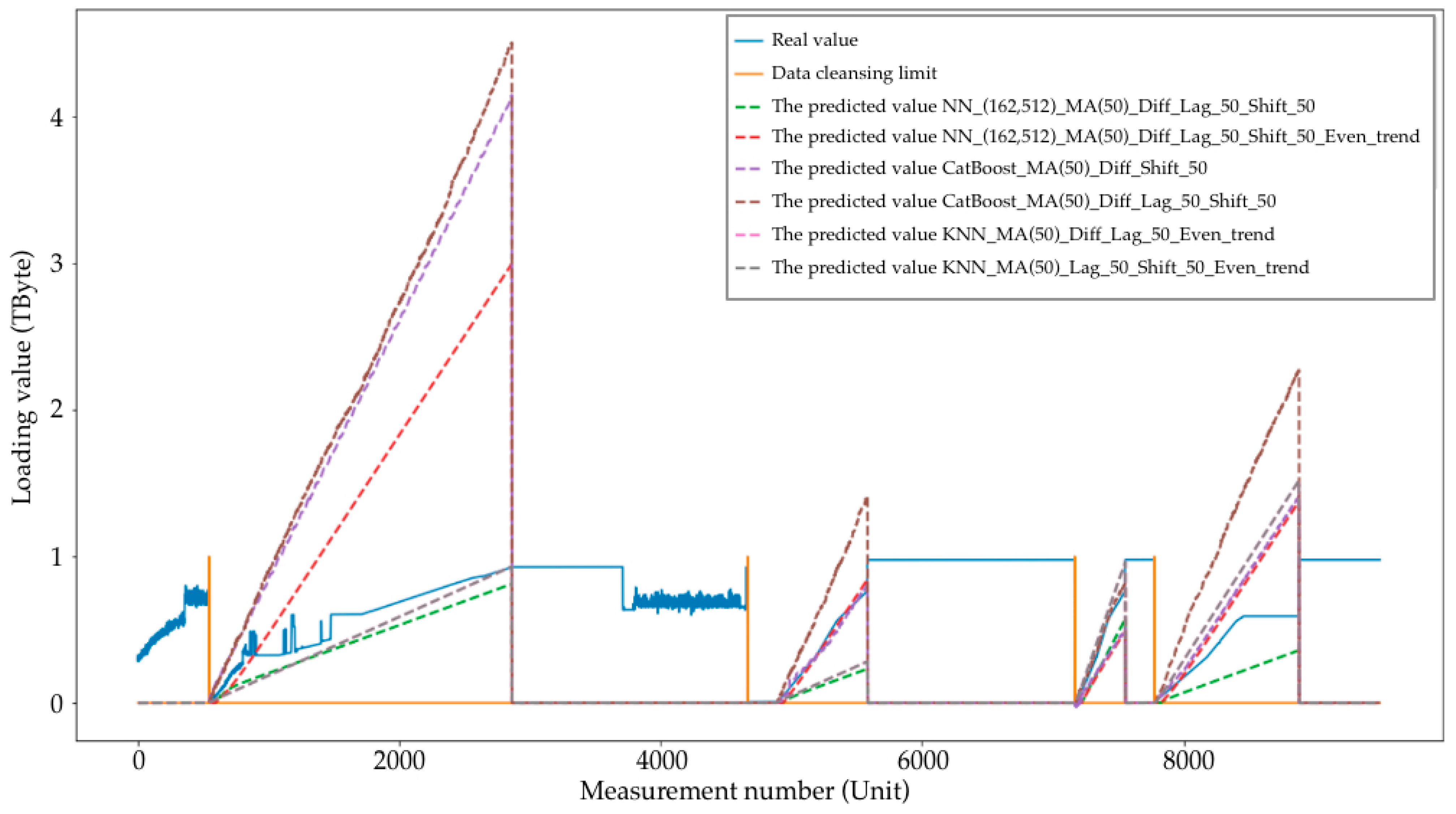
  • NN_(162,512)_MA(50)_Diff_Lag_50_Shift_50:
    Multilayer Perspectron Neural Network;
    Architecture: 2 hidden layers, namely, 1-162 and 2-512;
    Input parameters:
    MA (50);
    Diff (50)—50 observations back from the current value.
    From the starting point of the loading stage, 50 observations were “waited out” and the forecast was performed based on their values (this stage was performed only for the graph in Figure 8).
  • NN_(162,512)_MA(50)_Diff_Lag_50_Shift_50_Even_trend:
    Multilayer Perspectron Neural Network;
    Architecture—2 hidden layers: 1-162 and 2-512;
    The dataset for training was preprocessed to fully linear loading plots;
    Input data:
    MA (50);
    Diff (50)—50 observations back from the current value.
    From the starting point of the loading stage 50 observations were “waited out” and the forecast was performed based on their values (this stage was performed only for the graph in Figure 8).
  • CatBoost_MA(50)_Diff_Shift_50:
    CatBoostRegressor model;
    Hyperparameters by default;
    Input data:
    MA (50);
    Diff;
    From the starting point of the loading stage 50 observations were “waited out” and the forecast was performed based on their values (this stage was performed only for the graph in Figure 8).
  • CatBoost_MA(50)_Diff_Lag_50_Shift_50:
    CatBoostRegressor model;
    Hyperparameters by default;
    Input data:
    MA (50);
    Diff (50)—50 observations back from the current value.
    From the starting point of the loading stage 50 observations were “waited out” and the forecast was performed based on their values (this stage was performed only for the graph in Figure 8).
  • KNN_MA(50)_Diff_Lag_50_Even_trend:
    KNeighborsClassifier model;
    Hyperparameters:
    metric = ‘cityblock’;
    weights = ‘distance’.
    The dataset for training was preprocessed into fully linear loading sections;
    Input data:
    MA (50);
    Diff (50)—50 observations back from the current value.
  • KNN_MA(50)_Lag_50_Shift_50_Even_trend:
    KNeighborsClassifier model;
    Hyperparameters:
    metric = ‘cityblock’;
    weights = ‘distance’.
    The dataset for training was preprocessed into fully linear loading sections;
    Input data:
    MA (50);
    Diff (50)—50 observations back from the current value.
    From the starting point of the loading stage 50 observations were “waited out” and the forecast was performed based on their values (this stage was performed only for the graph in Figure 8).
After a comparative results analysis, we can conclude that the best result for the forecast of the full loading phase is the KNN_MA(50)_Diff_Lag_50_Even_trend model, shown in Figure 9.
Figure 9. The best model. KNN_MA(50)_Diff_Lag_50_Even_trend.
Electronics 11 04150 g009

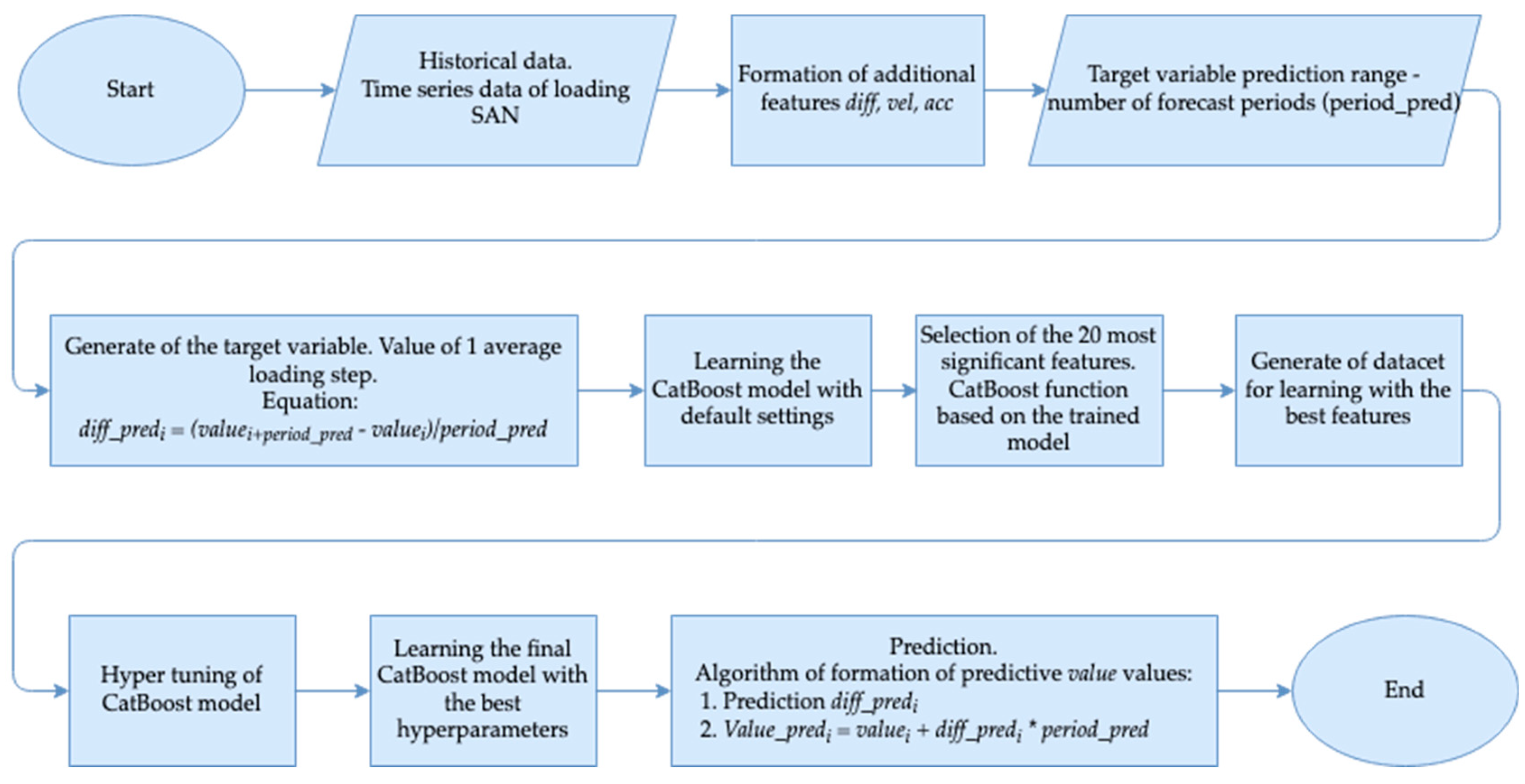
3.2. CatBoost Description

The CatBoost algorithm developed by Yandex is available through open access and is an algorithm consisting of gradient boosting applied to decision trees [21]. It is widely used in prediction tasks, such as weather forecasting or driving an unmanned car. Another example of the use of this algorithm is the prediction of the bankruptcy of a company; accordingly, the authors of [22] used CatBoost with only financial or qualitative variables for prediction and training, which were performed using a sample of data from about 90,000 organizations. This library implements a learning algorithm on the GPU and a scoring algorithm on the CPU, which greatly accelerates its performance; thus, the authors of article [23] conducted a direct comparison of other algorithms with CatBoost. The test was performed as follows: for each algorithm, a python test dataset was loaded; then, it was converted to the internal representation of the algorithm and the simulation time of the predictions was measured. The results showed that with the same ensemble size, CatBoost could run about 25 times faster than XGBoost and about 60 times faster than LightGBM.
In their work, Jabeur S. B. et al. [24] use gradient enhancement method to predict the bankruptcy of firms, which is a fundamental factor regarding banks’ decisions to lend money to organizations. The method used showed its high efficiency, which was proven by conducting a comparison with eight benchmark machine learning models one, two, and three years before the failure.
In [25], algorithms were proposed to solve the problem of prediction bias caused by a special kind of target leakage. These algorithms, implemented via CatBoost, include an implementation of ordered boosting, a permutation-based alternative to the classical algorithm, and an innovative algorithm for processing categorical features. The results show that the proposed algorithms solve the prediction shift problem efficiently, which leads to excellent empirical results.
The authors of [26] conducted a study on the sentimental analysis of social network messages on COVID-19 data using the CatBoost algorithm. The main purpose of this study was to determine the messages’ emotional tone and classify the messages. There was also a comparative study of different machine learning algorithms, and the results of performance indicators were illustrated graphically.
The CatBoost algorithm has gained wide applicability in medicine as well, as the authors of [27] developed their own methodology for the self-treatment of obesity, which allows one to create a personalized, optimal life plan that is easy to implement and adhere to, thereby reducing the incidence of obesity and obesity-related diseases.
Thus, it seems possible to judge the applicability of this algorithm for the task of SAN prediction.

4. Results

4.1. Initial Data Synthesis

In order to conduct broader research on SAN load prediction, the selection of models and methods and parameter tuning were conducted, and an artificial dataset implementation method was used, on which further experiments were subsequently conducted.
In addition, when applying the SAN load prediction system to real processes, the problem of raw data scarcity is encountered. This may arise due to the upgrade or implementation of a new storage area network or simply a lack of records for past periods of system operation. In such cases, it is proposed to use a prediction system pre-trained on artificial data and to then conduct additional training procedures on the observed data.
The SAN performance observations for various organizations show different schedules regarding storage occupancy over time. Some are linear, while others are more variable and less predictable. As mentioned above, a typical SAN utilization schedule contains distinct periods of increased utilization, periods of downtime, and periods of dramatic decreases in utilization. In general, a period of load growth consists of smaller characteristic areas, as illustrated in Figure 10.
The symbols on the graph in Figure 10:
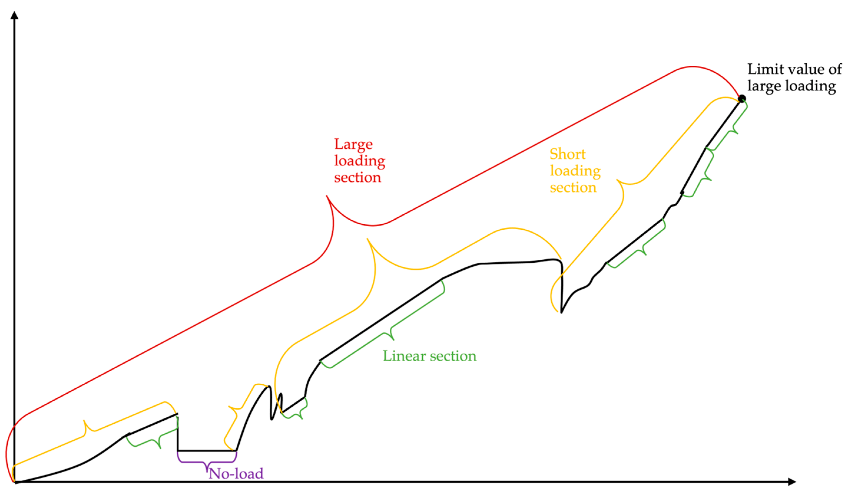
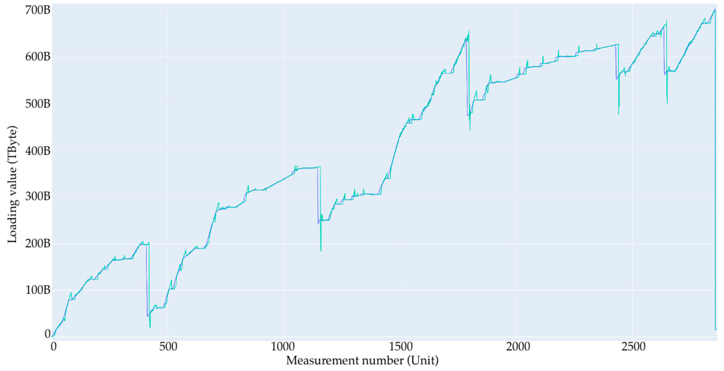
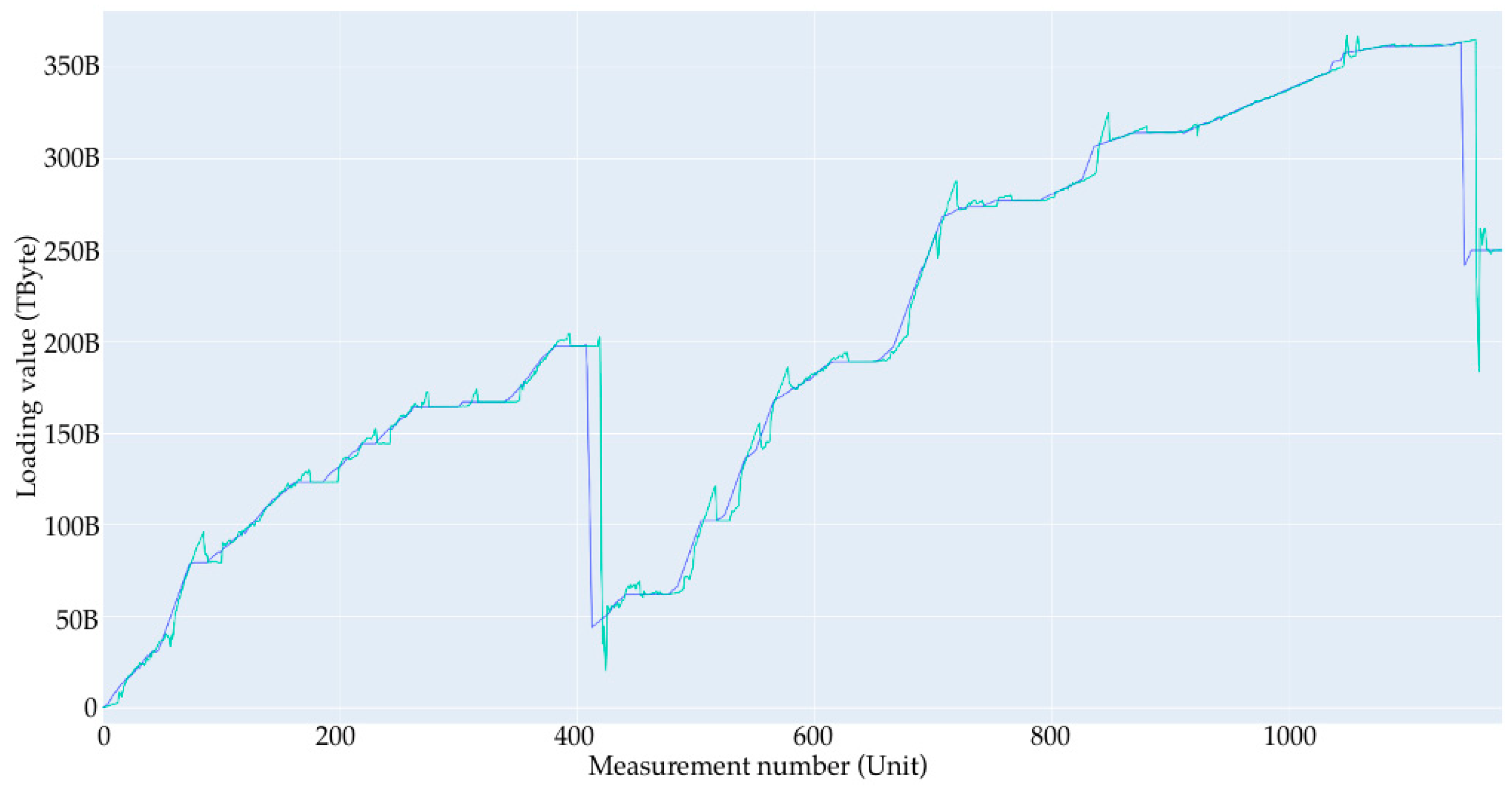
  • A large loading section (or large loading stage) is a storage area network loading from 0 to some limit value. In the case of the current data synthesis, the limit value is in the range of 60 to 90% of the total volume. In the current example, the volume is set to 1 Tb. After each large loading step, there is a complete deletion of records to 0 with no small deletion steps. Since the data are generated, the large loading steps are not related to each other, and this deletion is performed only to start a new loading step from a point at 0.
  • Short loading section (or small loading stage)—this is a local loading stage, similar to the large one, only inside of it. It is loaded at a smaller percentage, and after stage-by-stage deletion occurs with a simulation of the real values, it obtains one record of removal in the range from 10 Gb to 50 Gb; the range of the limits of removal are from 5 to 25% of the total volume.
  • No-load—this is the point at which nothing happens; the value is the same throughout several records.
  • Linear section—this is the section that is very close to the linear load, wherein the values of the increment at each step are in the range of ±5% of the average value given for this linear section to move from point A to point B.
Figure 11 shows a block diagram of the algorithm that allowed for the formation of a synthetic dataset for its further use in SAN load prediction. At the first stage, the algorithm is called through the configuration function, which contains a valid range of values, and through the number of examples function, which implies one large loading step.
Next, the condition is fulfilled if the number of examples is greater than zero; if so, the following information is determined:
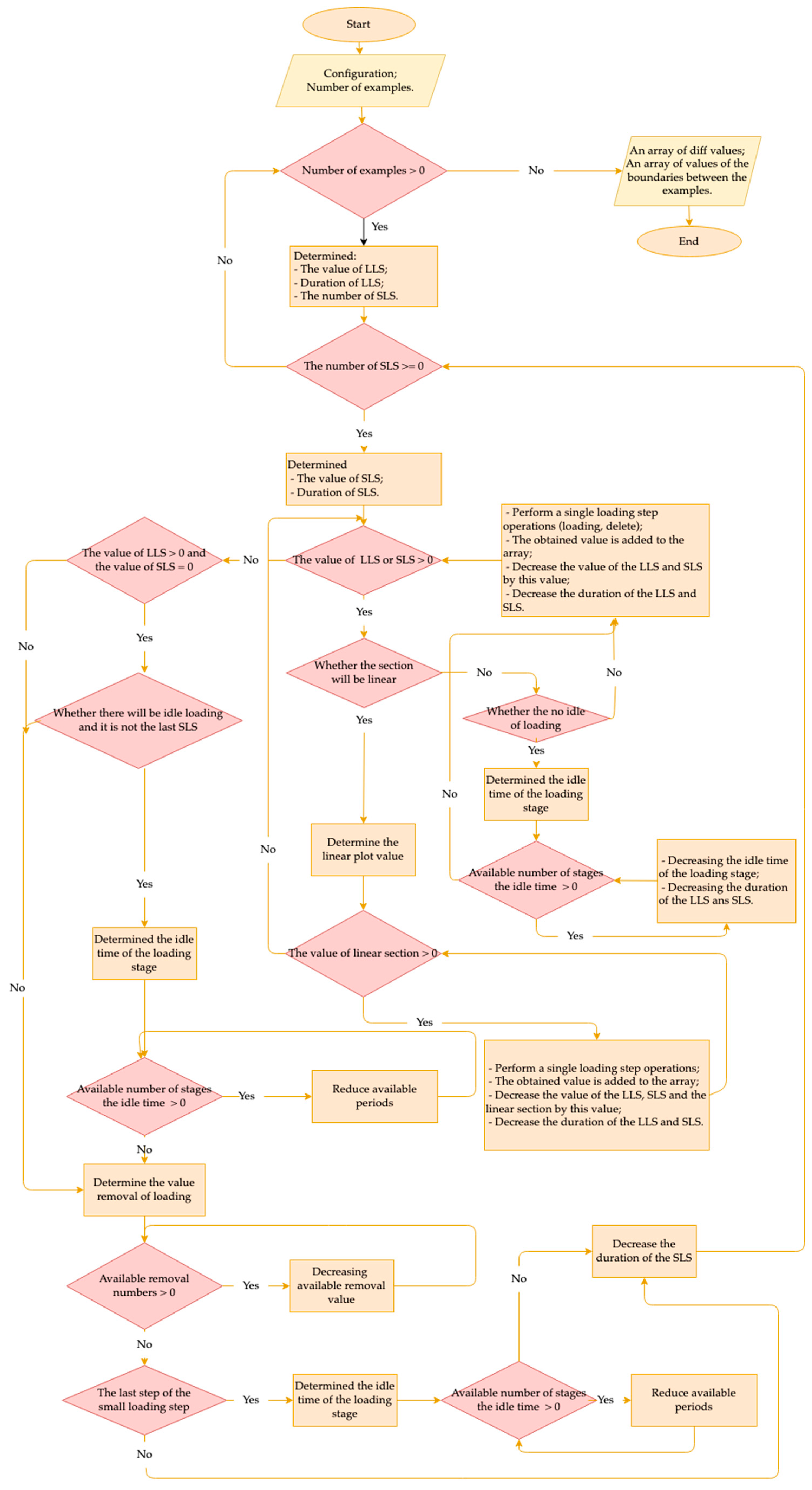
  • The value and duration of one large loading step (LLS);
  • The number of small loading steps (SLS), inside of the large one.
If this condition is not satisfied, the function with parameters is called:
  • An array of diff values (delta function);
  • An array of values of the boundaries between the examples;
  • The completion of the algorithm.
Then, in the case of a cycle, another cycle is started, as long as the value of the large loading step is greater than zero. At each iteration, the loading value is adjusted (if the loading increases, it decreases; if data are deleted, it increases), until this value is not equal to zero. In addition, the duration of loading is decreased.
Afterwards, the cycle is executed until the number of small loading steps is greater than zero or equals. The cycle determines the value and duration of the small loading step.
Then, the cycle is executed until the value of the small loading step is greater than zero. At the current stage, the loading value of each iteration is adjusted (if loading increases, then it decreases; if data are deleted, then it increases) until this value is 0, or until the value of the large stage is 0. In addition, the loading duration is decreased.
If the value of a large loading step or a small loading step is greater than zero, it is checked whether the section will be linear, that is, its probability of occurrence. The chance constant is set in the configuration; then, the value of the linear section is determined until it is less than zero, and the following steps are performed:
  • The operation of determining a single loading step is performed;
  • The obtained value is added to the array;
  • The values of the large loading step, the small loading step, and the linear section are decreased by this value;
  • The durations of the large loading step and the small loading step are decreased.
This cycle is performed as long as the section is linear. If the section is not linear, then it is checked whether there will be idle loading and its duration, and the following steps are performed as long as the available number of idle periods is less than or equal to zero:
  • the value of the large loading step, small loading step, and linear section are decreased by that value;
  • The durations of the large loading step and the small loading step are decreased.
Note that random selection is used. The chance constant for downtime is set in the configuration.
Provided that there is no idle time, the plot is not linear, and the small loading step is zero, an exit from the loop is performed and the loop is continued when the value of the large loading step is greater than zero and the small loading step is equal to zero. Then, the cycle is started while the idle time is greater than 0 and it is checked for the last stage of the small loading stage; consequently, the idle time of the loading stage is determined. Then, the cycle number of idle periods greater than zero is executed, where the available number of periods is reduced.
When the number of idle periods is less than or equal to zero, the cycle is exited. When the small loading stage has exhausted the value limit, the degree of data deletion is determined.
Then, if the limit of the large loading step is exhausted, the cycle is exited. After that, the cycle is executed until the deletion value is greater than zero, in which case the available value decreases.
The next step executes the cycle until the last step of the small loading step. This step determines the idle duration of the load, and then executes the cycle until the idle duration is greater than zero. In this case, it is determined whether there will be idle loading (no increment) after deleting the data in the small stage. Random selection is used. The chance constant, i.e., that there will be downtime, is set in the configuration. It is worth undoing this step when the small loading stage has exhausted the value limit, then the degree of data deletion is determined.
When the deletion value is greater than zero and the limit of the small loading step is exhausted, then the transition to the loop execution step is finished, while the number of examples is greater than 0.
If this condition is not met, the function returns two data arrays:
  • An array of delta values;
  • An array of boundary values between examples.
The values of the parameters used in the formation of synthetic data are shown in Table 2.
Examples of the resulting synthetic data are shown in Figure 12.

4.2. Formation of a Set of Essential Features for Predicting SAN Utilization

A simulation of the dataset sections that contain periods of loading, deleting data, and downtime was performed. The time interval in the original data is 5 min.
Initially, to select the best model, the difference between the data growth and volume was used to determine attributes; thus, the variable “Deviation” (diff) is the difference between the current value of SAN loading and the previous one. The planning horizon (the period of time for which SAN utilization should be predicted) takes values of 1 h, 2 h, 4 h, 8 h, 24 h, and 48 h.
The input data in the problem under consideration are the volume load values at different moments of time, where the time interval of records is 5 min.
v0, v1, v2, …, where v0 is the workload at the present moment of time for which further workload is predicted, and vi is the known workload at moment ti units of time earlier.
As it was described earlier, this study’s problem is considered as the problem of predicting the load increase from the current moment of time to some period in the future, diff* = v* − v0, where v* is the predicted load at moment t*.
As inputs we also used the load increases in the previous time periods ti calculated on the basis of the initial data: diffi = vivi−1.
As the experiments show, the influence of the diffi attributes turns out to be insignificant, especially when i increases.
The following hypotheses were formulated in order to ascertain the set of significant attributes and to build a prediction model.
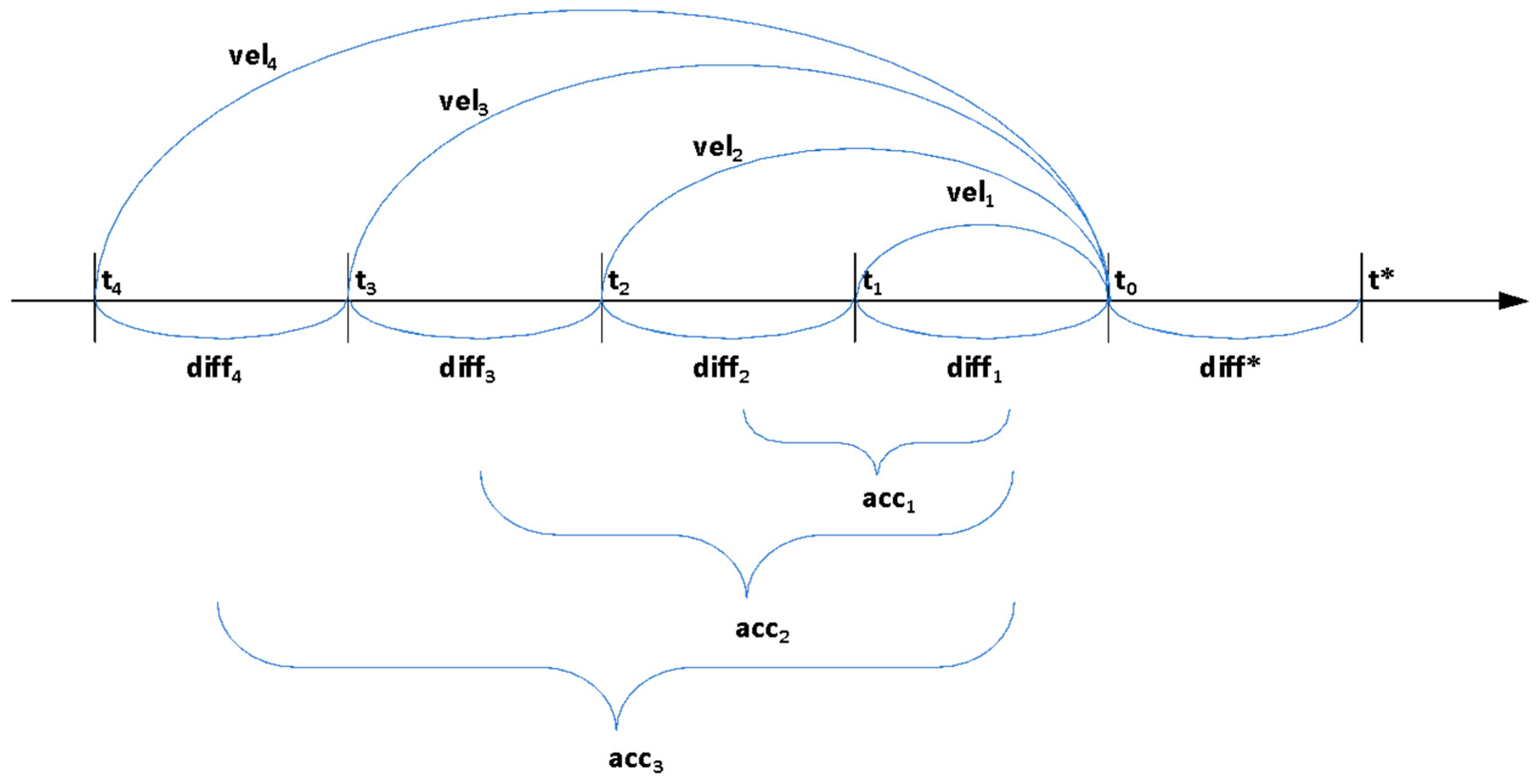
  • The value of load increase in the next period of time is close to the current value of load increase diff1 (the principle of “inertia” or stable load increase);
  • In the case when the change of the diff value at the current moment is temporary, and when the value of diff was higher or lower during the entirety of the earlier operation, then the average value of loading change at time periods (tj, tj−1, …, t1), j = 1, …, n) should be considered (the principle of the “average speed” of loading corresponds to Equation (1)):
v e l j = 1 j i = 1 j   d i f f i ,
3.
In the case when the loading rate (vel) increases (or decreases) in the process, then this tendency to increase (decrease) should be considered with respect to the values of the change in diff (the principle of accounting for the “acceleration” of the loading is given in Equation (2)):
a c c j = 1 j i = 1 j   d i f f i d i f f i + 1 ,
Thus, it is proposed to use the values velj and accj as input attributes (Figure 13).
Table 3 shows a fragment of the preprocessed dataset. Only the most important fields are shown.

4.3. Experimental Results

All experiments were performed on the CatBoostRegressor model with basic settings.
Experiment No. 1 (Table 4).
  • The model was tested on 576 incoming diff properties.
  • The 10 best properties were selected by the CatBoost model function “get_feature_importance”. Testing was conducted on these properties.
  • The five best properties were selected by the CatBoost model function “get_feature_importance”. Testing was conducted on these properties.
  • The three best properties were selected by the function of the CatBoost model “get_feature_importance”. Testing was conducted on these properties.
  • A single best property was selected by the CatBoost model function “get_feature_importance”. Testing was conducted on these properties.
Definition of the variable diff:
Diff is the difference between the current value and the previous value. For example, if line number 10 is selected, then let us assume that diff5 is equal to the value of line 5 minus the value of line 4, that is, the values of the previous entries. For instance, if it is now 13:00, then we know the values for 12:00, 11:00, 10:00, and so on. These functions are fed to the input of the model.
Based on the results of this test, we can conclude that the three incoming diff properties give the best results on the MAE metric.
Experiment No. 2 (Table 5).
  • Testing was performed on 1151 incoming properties. Of these:
    • Average velocity (vel)—576;
    • Average acceleration (acc)—575.
  • The 20 best properties were selected by the CatBoost model function “get_feature_importance”. Tests were conducted on these properties.
  • The 10 best properties were selected by function of the CatBoost model “get_feature_importance”. Tests were conducted on these properties.
  • The five best properties were selected by the function of the CatBoost model “get_feature_importance”. Tests were conducted on these properties.
From the results of this experiment, we can conclude that the best results were obtained for 1151 incoming properties, but this requires a long learning curve for the model. This option is not suitable for finding the optimal model. It is better to search for the optimal model applied to the top 20 properties. However, the optimal model can already be trained on all properties.
The following conclusions have been drawn from these studies:
  • Changing the feature space by introducing the generalizing features velj and accj leads to improved prediction;
  • A truncated feature set simplifies the model and accelerates training without incurring a significant loss (or improvement) of prediction accuracy.
Subsequently, the most significant 20 attributes consisting of the average rates and acceleration rates of load growth were used to build the forecasting model.
A general block diagram of the prediction algorithm is shown in Figure 14.

5. Experimental Studies on Predicting SAN Loading Using Regression

5.1. Predicting SAN Utilization by Regression One Hour Ahead

The following models and parameters were used for the regression task:
  • CatBoostRegressor and CatBoost Library;
  • KNeighborsRegressor, using the k-nearest neighbor method;
  • LinearRegression, linear regression.
  • CatBoost model hyperparameter grid search:
  • Loss-function MAE average absolute error;
  • A test sample size of 20%.
  • The following is a list of CatBoost model hyperparameters:
‘learning_rate’: [0.03, 0.04, 0.05, 0.06, 0.07, 0.08, 0.09],
‘depth’: [10, 11, 12],
‘l2_leaf_reg’: [2, 3, 4, 5, 6, 7, 8],
‘bootstrap_type’: [‘Bernoulli’, ‘Bayesian’, ‘MVS’, ‘No’]
  • The best hyperparameters of the CatBoost model are as follows:
‘iterations’: 1000,
‘loss_function’: ‘MAE’,
‘random_seed’: 42,
‘verbose’: False,
‘boosting_type’: ‘Plain’,
‘task_type’: ‘CPU’,
‘depth’: 9,
‘l2_leaf_reg’: 2,
‘learning_rate’: 0.09,
‘bootstrap_type’: ‘Bernoulli’}
LinearRegression model on the top 20 attributes, with a test sample size of 20%:
DIFF train:
R2 0.11759055044319466
mean_absolute_error 368.54792226600927 5 min/Mb
DIFF test:
R2 0.1032108082741724
mean_absolute_error 391.8978915286052 5 min/Mb
Value train:
R2 0.9953090618853814
mean_absolute_percentage_error 48.447349557246284%
Value test:
R2 0.994880793879479
mean_absolute_percentage_error 57.711763654202244%
KNeighborsRegressor model hyperparameter grid search on top-20 features
  • The best hyperparameters of the KneighborsRegressor model are as follows:
‘metric’: ‘cityblock’,
‘n_neighbors’: 110,
‘weights’: ‘uniform’}
The results of different variants of the test sample size are as follows:
DIFF train:
R2 0.21459744816203896
mean_absolute_error 332.0943812516901 5 min/Mb
DIFF test:
R2 0.1768628775777361
mean_absolute_error 296.16665025915586 5 min/Mb
Summary results of the regression models are shown in Table 6.
We can conclude the following findings on forecasting with regression models: according to the MAE metric, which provided the average absolute error, the best regression model is CatBoost.

5.2. Predicting SAN Load Using Neural Networks

Table 7 (Model: “sequential_5”) shows the structures of the neural networks used.
The results of applying the neural network are presented below.
DIFF train:
R2 0.09572336879029608
mean_absolute_error 267.88508843588266 5 min/Mb
DIFF test:
R2 0.0715112658919046
mean_absolute_error 293.7732381006516 5 min/Mb
Value train:
R2 0.9951645323227666
mean_absolute_percentage_error 48.22053331531325%
Value test:
R2 0.9946512741134749
mean_absolute_percentage_error 56.9436754761519%
A summary of the results of the neural network application is shown in Table 8.
According to the MAE, i.e., the average absolute error metric, the best neural network architecture is 10 hidden layers with 30 neurons each. However, the metrics of this neural network are worse than those of the CatBoost model.
A visualization of the forecast for 1 h and real data on the graph of the CatBoost model are shown in Figure 15.
The graph (Figure 15) was constructed from one large loading stage. The graph (Figure 14) shows the entire loading step; the next graph (Figure 16) shows one part of it with a larger scale.
The formula for calculating the predicted values on the graph:
Value_predicti = valuei-12 + diff_predicti-12 * 12
where value_predict is the point to be predicted (the value in 12 records from the current time or 1 h).
Value is the current volume load value.
Diff_predict is the predicted average value of the load gain or loss, which must be added to the current value 12 times to predict the load value in 1 h.
Note: The model predicts only 1 point in 1 h, wherein the way to this point is a straight line from the average diff. The curvature of the forecast on the graph was already verified from the previous forecasts.

5.3. Predicting SAN Load Using Regression for 24 h Ahead

Using the conclusions of Section 6and Section 7 concerning the choice of the best model for predicting SAN utilization one hour ahead, let us consider the use of CatBoost for a 24 h forward forecast.
  • CatBoost hyperparameter grid search on top—20 parameters.
  • The list of hyperparameters of the CatBoost model:
‘learning_rate’: [0.03, 0.04, 0.05, 0.06, 0.07, 0.08, 0.09],
‘depth’: [1, 2, 3, 4, 5, 6, 7, 8, 9],
‘l2_leaf_reg’: [2, 3, 4, 5, 6, 7, 8],
‘bootstrap_type’: [‘Bernoulli’, ‘Bayesian’, ‘MVS’, ‘No’
  • The best hyperparameters of the CatBoost model:
‘iterations’: 200,
‘loss_function’: ‘MAE’,
‘random_seed’: 42,
‘verbose’: False,
‘boosting_type’: ‘Plain’,
‘task_type’: ‘CPU’,
‘depth’: 9,
‘l2_leaf_reg’: 6,
‘learning_rate’: 0.05,
‘bootstrap_type’: ‘Bernoulli’
  • The best results of the CatBoost model prediction:
DIFF train:
R2 0.3517532239354847
mean_absolute_error 160.15495056506484 5 min/Mb
DIFF test:
R2 0.19196146687069315
mean_absolute_error 194.37242886618847 5 min/Mb
Value train:
R2 0.8578543459067921
mean_absolute_percentage_error 807.5265537419783%
Value test:
R2 0.8113079668072851
mean_absolute_percentage_error 682.4150839712811%
The CatBoost model is shown in Figure 17 in a visualization of the 24 h forecast and real data on a graph.
The graph (Figure 17) is built from one large loading stage. The graph (Figure 17) shows the whole loading phase, while the next graph (Figure 18) shows one part of it at a larger scale.
The formula for calculating the predicted values on the graph:
Value_predicti = valuei-288 + diff_predicti-288 * 288
where value_predict is the point to predict (value in 288 records from the current time or 24 h).
Value is the current value of volume load.
Diff_predict is the predicted average value of the load gain or loss, which must be added to the current value 288 times to predict the load value in 24 h.
Note: The model predicts only 1 point in 24 h; the way to this point is a straight line from the average diff. The curvature of the forecast on the graph is already a fact of previous forecasts.
Table 9 presents comparisons of the predictions of all target variables.

6. Discussion

To perform detailed experiments on the considered problem of SAN load prediction, an artificial data set was generated, which corresponds to the real data on SAN load measurements, including periods of growth, idle time, and volume cleaning.
The CatBoost algorithm (decision-tree gradient binning) showed a higher efficiency compared to other regression analysis algorithms (linear regression, nearest neighbor, and artificial neural networks) in terms of the R2_score and MAE.
The use of generalizing features—such as the “average loading speed” and “average loading acceleration”, which were introduced in accordance with the hypotheses of their influence on further growth—in the CatBoost algorithm for regression led to an increase in the prediction accuracy by 30% on average. The identification and selection of the most significant attributes in the CatBoost algorithm allows for the simplification of the forecast model almost without a loss (and, in some cases, producing an increase) in the forecast’s accuracy, thereby reducing the number of used attributes to 20.
The prediction accuracy decreases slightly when the planning horizon increases. Thus, when planning for 1 h, the R2 is close to 1; when planning for 8 h, the R2 is approximately equal to 0.95; but when planning for 24 h and more, the R2 decreases to 0.9 and lower. Nevertheless, the proposed approach is quite applicable for practical SAN utilization prediction based on the records of previous utilization states.

7. Conclusions

The artificial data set synthesized stochastically according to the specified parameter intervals allowed us to conduct more extensive experiments. In general, the synthesized data correspond to real data, which allows for the generalization of the results of the experimental studies. In addition, the pre-trained model can be applied in cases where historical data are extremely scarce. In this case, the use of a pre-trained model on synthetic data is a useful technique. In further SAN work, this model will be further trained according to real measurements.
The best model for prediction is the CatBoost model. Adding generalizable features, such as the SAN load speed (vel) and the SAN load acceleration (acc), improves its prediction. A truncated set of features consisting of up to 20 attributes simplifies the model and accelerates training without a significant loss of prediction accuracy. The best results are obtained when predicting up to about 100 records ahead, and then the accuracy decreases. However, the results can be improved by training the model on real data concerning specific equipment.
For practical applications, a graphical user interface (GUI) application for SAN utilization prediction based on the best-trained CatBoost model has been developed based on this research.

Author Contributions

Conceptualization, I.S.M., V.S.T., V.A.N., V.V.B., S.O.K., A.P.G. and A.S.B.; methodology, I.S.M., V.S.T., V.A.N., V.V.B. and S.O.K.; software, I.S.M. and A.P.G.; validation, I.S.M., V.S.T., V.A.N. and V.V.B.; formal analysis, V.A.N., V.V.B., S.O.K. and A.P.G.; investigation, I.S.M., V.S.T., V.A.N. and V.V.B.; resources, V.A.N., V.V.B., S.O.K. and A.P.G.; data curation, I.S.M., V.S.T., V.A.N. and V.V.B.; writing—original draft preparation, I.S.M., V.S.T., V.A.N., V.V.B., S.O.K. and A.P.G.; writing—review and editing, I.S.M., V.S.T., V.A.N., V.V.B., S.O.K., A.P.G. and A.S.B.; visualization, I.S.M., V.S.T., V.A.N., A.P.G. and A.S.B.; supervision, V.A.N., V.V.B. and S.O.K.; project administration, I.S.M., V.S.T., V.A.N., V.V.B. and A.S.B.; funding acquisition, V.S.T., V.A.N. and A.S.B. All authors have read and agreed to the published version of the manuscript.

Funding

The studies were carried out within the program of the Russian Federation of strategic academic leadership “Priority-2030” aimed at supporting the development programs of educational institutions of higher education, the scientific project PRIOR/SN/NU/22/SP5/16 “Building intelligent networks, determining their structure and architecture, operation parameters in order to increase productivity systems and the bandwidth of data transmission channels using trusted artificial intelligence technologies that provide self-learning, self-adaptation, and optimal reconfiguration of intelligent systems for processing large heterogeneous data”.

Institutional Review Board Statement

Not applicable.

Informed Consent Statement

Not applicable.

Data Availability Statement

Not applicable.

Conflicts of Interest

The authors declare no conflict of interest.

References

  1. Çelik, D.; Meral, M.E.; Waseem, M. Investigation and Analysis of Effective Approaches, Opportunities, Bottlenecks and Future Potential Capabilities for Digitalization of Energy Systems and Sustainable Development Goals. Electr. Power Syst. Res. 2022, 211, 108251. [Google Scholar] [CrossRef]
  2. Waseem, M.; Lin, Z.; Liu, S.; Jinai, Z.; Rizwan, M.; Sajjad, I.A. Optimal BRA Based Electric Demand Prediction Strategy Considering Instance-Based Learning of the Forecast Factors. Int. Trans. Electr. Energy Syst. 2021, 31, e12967. [Google Scholar] [CrossRef]
  3. Teggi, P.; Malakreddy, B.; Teggi, P.P.; Harivinod, N. AIOPS Prediction for Server Stability Based on ARIMA Model. Int. J. Eng. Tech. Res. 2021, 10, 128–134. [Google Scholar]
  4. Nääs Starberg, F.; Rooth, A. Predicting a Business Application's Cloud Server CPU Utilization Using the Machine Learning Model LSTM. DEGREE Proj. Technol. 2021, 1, 1–14. [Google Scholar]
  5. Nashold, L.; Krishnan, R. Using LSTM and SARIMA Models to Forecast Cluster CPU Usage. arXiv 2020. [Google Scholar] [CrossRef]
  6. D’souza, R. Optimizing Utilization Forecasting with Artificial Intelligence and Machine Learning. Available online: https://www.datanami.com/2020/ (accessed on 21 October 2022).
  7. Masich, I.S.; Tyncheko, V.S.; Nelyub, V.A.; Bukhtoyarov, V.V.; Kurashkin, S.O.; Borodulin, A.S. Paired Patterns in Logical Analysis of Data for Decision Support in Recognition. Computation 2022, 10, 185. [Google Scholar] [CrossRef]
  8. Yoas, D.W. Using Forecasting to Predict Long-Term Resource Utilization for Web Services. Ph.D. Thesis, Retrieved from NSUWorks, Graduate School of Computer and Information Sciences. Nova Southeastern University, Lauderdale, FL, USA, 2013. [Google Scholar]
  9. Mikhalev, A.S.; Tynchenko, V.S.; Nelyub, V.A.; Lugovaya, N.M.; Baranov, V.A.; Kukartsev, V.V.; Sergienko, R.B.; Kurashkin, S.O. The Orb-Weaving Spider Algorithm for Training of Recurrent Neural Networks. Symmetry 2022, 14, 2036. [Google Scholar] [CrossRef]
  10. Cheong, C.W.; Way, C.C. Fuzzy Linguistic Decision Analysis for Web Server System Future Planning. In Proceedings of the IEEE Region 10 Annual International Conference (TENCON), Kuala Lumpur, Malaysia, 24–27 September 2000; Volume 1, pp. 367–372. [Google Scholar]
  11. Cheong, C.W.; Hua, K.Y.W.; Leong, N.K. Web Server Future Planning Decision Analysis—Fuzzy Linguistic Weighted Approach. In Proceedings of the 4th International Conference on Knowledge-Based Intelligent Engineering Systems and Allied Technologies (KES 2000), Brighton, UK, 30 August–1 September 2000; Volume 2, pp. 826–830. [Google Scholar]
  12. Khosla, N.; Sharma, D. Using Semi-Supervised Classifier to Forecast Extreme CPU Utilization. Int. J. Artif. Intell. Appl. 2020, 11, 45–52. [Google Scholar] [CrossRef]
  13. Tatarnikova, T.M.; Poymanova, E.D. Differentiated Capacity Extension Method for System of Data Storage with Multilevel Structure. Sci. Tech. J. Inf. Technol. Mech. Opt. 2020, 20, 66–73. [Google Scholar] [CrossRef] [Green Version]
  14. Poimanova, E.D.; Tatarnikova, T.M.; Kraeva, E.V. Model of Data Traffic Storage Management. J. Instrum. Eng. 2021, 64, 370–375. [Google Scholar] [CrossRef]
  15. Sovetov, B.Y.; Tatarnikova, T.M.; Poymanova, E.D. Storage Scaling Management Model. Inf.-Upr. Sist. 2020, 1, 43–49. [Google Scholar] [CrossRef]
  16. Janardhanan, D.; Barrett, E. CPU Workload Forecasting of Machines in Data Centers Using LSTM Recurrent Neural Networks and ARIMA Models. In Proceedings of the 2017 12th International Conference for Internet Technology and Secured Transactions (ICITST), Cambridge, UK, 11–14 December 2017; pp. 55–60. [Google Scholar]
  17. Tran, V.G.; Debusschere, V.; Bacha, S. Hourly Server Workload Forecasting up to 168 Hours Ahead Using Seasonal ARIMA Model. In Proceedings of the 2012 IEEE International Conference on Industrial Technology (ICIT), Athens, Greece, 19–21 March 2012; pp. 1127–1131. [Google Scholar]
  18. Zharikov, E.; Telenyk, S.; Bidyuk, P. Adaptive Workload Forecasting in Cloud Data Centers. J. Grid Comput. 2020, 18, 149–168. [Google Scholar] [CrossRef]
  19. Baldan, F.J.; Ramirez-Gallego, S.; Bergmeir, C.; Herrera, F.; Benitez, J.M. A Forecasting Methodology for Workload Forecasting in Cloud Systems. IEEE Trans. Cloud Comput. 2018, 6, 929–941. [Google Scholar] [CrossRef]
  20. Tran, V.G.; Debusschere, V.; Bacha, S. Neural Networks for Web Server Workload Forecasting. In Proceedings of the 2013 IEEE International Conference on Industrial Technology (ICIT), Cape Town, South Africa, 25–28 February 2013; pp. 1152–1156. [Google Scholar]
  21. CatBoost. Available online: https://catboost.ai/ (accessed on 20 October 2022).
  22. Yao, C.; Dai, Q.; Song, G. Several Novel Dynamic Ensemble Selection Algorithms for Time Series Prediction. Neural Process. Lett. 2019, 50, 1789–1829. [Google Scholar] [CrossRef]
  23. Dorogush, A.V.; Ershov, V.; Yandex, A.G. CatBoost: Gradient Boosting with Categorical Features Support. arXiv 2018. [Google Scholar] [CrossRef]
  24. Jabeur, S.B.; Gharib, C.; Mefteh-Wali, S.; Arfi, W.B. CatBoost model and artificial intelligence techniques for corporate failure prediction. Technol. Forecast. Soc. Change 2021, 166, 120658. [Google Scholar] [CrossRef]
  25. Prokhorenkova, L.; Gusev, G.; Vorobev, A.; Dorogush, A.V.; Gulin, A. CatBoost: Unbiased boosting with categorical features. In Proceedings of the 32nd Conference on Neural Information Processing Systems, NEURIPS 2018, Montreal, QC, Canada, 2–7 December 2018; Volume 31, pp. 6638–6648. [Google Scholar]
  26. Aarthi, B.; Jeenath Shafana, N.; Tripathy, S.; Sampat Kumar, U.; Harshitha, K. Sentiment Analysis Using CatBoost Algorithm on COVID-19 Tweets. Lect. Notes Data Eng. Commun. Technol. 2023, 131, 161–171. [Google Scholar] [CrossRef]
  27. Chen, S.; Dai, Y.; Ma, X.; Peng, H.; Wang, D.; Wang, Y. Personalized Optimal Nutrition Lifestyle for Self Obesity Management Using Metaalgorithms. Sci. Rep. 2022, 12, 12387. [Google Scholar] [CrossRef] [PubMed]
Figure 1. Provided dataset without preprocessing.
Electronics 11 04150 g001
Figure 10. Explanations of the used parameters on the example of the initial data graph.
Electronics 11 04150 g010
Figure 11. Block diagram of the synthetic dataset algorithm.
Electronics 11 04150 g011
Figure 12. Examples of synthetic data, where the red lines on the large loading steps are separated because they are separate and independent from the antecedents, wherein the measurement number is measured sequentially at a certain interval.
Electronics 11 04150 g012
Figure 13. Feature generation for the task of SAN load prediction.
Electronics 11 04150 g013
Figure 14. Block diagram of the entire prediction algorithm.
Electronics 11 04150 g014
Figure 15. Graph of the forecast for 1 h and real data on the chart, for the CatBoost model, and in normal scale, where: blue—real value; turquoise—forecast value based on the CatBoost model.
Electronics 11 04150 g015
Figure 16. Graph of the forecast for 1 h and real data on the graph, using the CatBoost model, and in enlarged scale, where: blue—the real value; turquoise—the forecast value based on the CatBoost model, where measurement number is measured sequentially at a certain interval.
Electronics 11 04150 g016
Figure 17. Graph of the forecast for 24 h and real data on the chart, using CatBoost model, and in normal scale, where: in blue—real value; in turquoise—forecast value based on the CatBoost model, where measurement number is measured sequentially at a certain interval.
Electronics 11 04150 g017
Figure 18. The graph of the forecast for 24 h and real data on the graph, using the CatBoost model, and in enlarged scale, where: in blue—the real value; in turquoise—the forecast value based on the CatBoost model.
Electronics 11 04150 g018
Table 2. Parameters for synthetic data generation.
ParametersMin.
Value
Max. Value
Limit value range of one large loading step (% of volume filling)6090
The duration of one large loading step (number of hours)192384
Range of values, i.e., the number of small loading steps within a large one07
Limit value range of one small loading step within a large one (% of volume filling)1050
Duration of one small download step within a large one (number of hours)848
Value range of one download record (5 min/Mb)1003500
One deletion record. Only considered when downloading (5 min/Mb)5001000
Probability of a deletion record appearing only when downloading (%)1
Limit value range of one deletion step. Follows a small loading step (% volume filling)525
Range of values of one deletion record. Only considered at the moment of large data cleaning (5 min/Mb)10,00050,000
Probability of a linear section appearing (approximation to the average value of the loading section) at a small loading step (%)1
Percentage of available values from the average in a linear segment5
Distance of a linear section in a small loading stage (ratio to the remaining value of a small loading stage) (%)1030
Length of time of no-volume loading after a small loading step (number of hours)130
Probability of occurrence of downtime after a small loading step (%)20
Duration of volume unloading absence at the moment of loading a small stage (number of hours)13
Probability of the absence of volume unloading at the time of downloading a small stage (%)1
Table 3. Processed dataset.
IndexValueDiffDiff_PredVel_1Vel_2Vel_4Acc_1Vel_3Vel_37Acc_3Acc_2
02.88 × 1082.88 × 1087.84 × 108287,595,4271.44 × 1087.18 × 1072.88 × 10895,865,14226,145,03995,865,1421.44 × 108
14.6 × 1081.73 × 1088.52 × 108172,849,9372.3 × 1081.15 × 108−1.1 × 1081.53 × 10838,370,44757,616,64686,424,969
21.46 × 1091098.74 × 1081,000,166,7795.87 × 1083.65 × 1088.27 × 1084.87 × 1081.12 × 1083.33 × 1083.56 × 108
31.69 × 1092.32 × 1089.11 × 108231,652,1346.16 × 1084.23 × 108−7.7 × 1084.68 × 1081.21 × 108−1.9 × 10729,401,099
41.93 × 1092.34 × 1089.47 × 108233,602,9122.33 × 1084.1 × 1081,950,7784.88 × 1081.28 × 10820,250,992−3.8 × 10⁸
53.09 × 1091.16 × 1098.87 × 1081,163,185,9056.98 × 1086.57 × 1089.3 × 1085.43 × 1081.93 × 10854,339,7094.66 × 108
64.23 × 1091.14 × 1098.45 × 1081,139,444,8411.15 × 1096.92 × 108−2.4 × 1078.45 × 1082.49 × 1083.03 × 1084.53 × 108
75.25 × 1091.02 × 1098.65 × 1081,022,942,8721.08 × 1098.9 × 108−1.2 × 1081.11 × 1092.92 × 1082.63 × 108−7 × 10⁷
86.23 × 1099.81 × 1088.04 × 108980,959,5921091.08 × 109−4.2 × 1071.05 × 1093.28 × 108−6.1 × 10⁷−7.9 × 10⁷
97.49 × 1091.26 × 1097.38 × 1081,258,057,2921.12 × 1091.1 × 1092.77 × 1081.09 × 1093.75 × 10839,537,4841.18 × 108
108.46 × 1099.65 × 1087.09 × 108964,858,1931.11 × 1091.06 × 109−2.9 × 1081.07 × 1094.03 × 108−1.9 × 10⁷−8,050,700
Table 4. Comparison table of the results of test #1 sorted by MAE.
FeatureR2_ScoreMAE (5 min/Mb)
top_3_diff0.141245.3
top_5_diff0.136245.518
top_10_diff0.118250.166
diff—diff5750.095251.993
top_1_diff0.141245.3
Table 5. Comparison table of the results of experiment #2 sorted by MAE.
FeatureR2_ScoreMAE (5 min/Mb)
vel576_acc_5750.158241.16
top_200.164243.976
top_100.166244.427
top_50.157245.122
Table 6. Ranking of the best regression models.
FeatureR2_Score_TestMAE (5 min/Mb) TestR2_Score_TrainMAE (5 min/Mb) TrainR2_Score_Value_TrainMAPE TrainR2_Score_TestMAPE_TestTime
0CatBoost0.170824278.8000980.208604246.2536020.99577641.6626290.99524747.19025160 s
1LinearRegression0.103211391.8978920.117591368.5479220.99530948.4473500.99488157.7117641 s
2KNeighborsRegressor0.181701316.1293830.215314290.1576080.99581441.7463530.99530247.815941240 s
Table 7. The architecture and metrics of the first neural network.
Layer (Type)Output ShapeParam #
dense_28 (Dense)(None, 256)5376
dense_29 (Dense)(None, 256)5376
dense_30 (Dense)(None, 256)65,792
dense_31 (Dense)(None, 256)65,792
dense_32 (Dense)(None, 256)65,792
dense_33 (Dense)(None, 256)65,792
dense_34 (Dense)(None, 256)65,792
dense_35 (Dense)(None, 256)65,792
dense_36 (Dense)(None, 256)65,792
dense_37 (Dense)(None, 256)65,792
dense_38 (Dense)(None, 1)257
Total params: 597,761
Trainable params: 597,761
Non-trainable params: 0
Table 8. Summary results of the application of neural networks.
featureR2_Score_TestMAE (5 min/Mb) TestR2_Score_TrainMAE (5 min/Mb) TrainR2_Score_Value_TrainMAPE TrainR2_Score_TestпpostTime
0NN (30)0.145156296.4603960.169836272.3149800.99556843.7991240.99509252.62516885 s
1NN 10 layers of 30 neurons0.132219291.1387130.165863265.0174110.99556140.6824880.99507950.087625100 s
2NN (256)0.143416300.9171260.166495277.0477180.99554646.4529040.99507255.71656080 s
3NN 10 layers of 256 neurons0.076478297.9205650.098162273.2988650.99517848.1495210.99468056.919627130 s
Table 9. Comparison table for predicting all target variables 1, 2, 4, 8, 24, 48 h.
ModelDiff Train MAEDiff Test MAEDiff Train R2Diff Test R2Value Train MAPEValue Test MAPEValue Train R2Value Test R2
1 h246.25277.80.210.1741.6647.190.9960.995
2 h275.22307.00.170.1290.63102.50.9890.988
4 h275.2300.620.180.12178.67217.260.9760.973
8 h240.15266.050.240.15348.02458.50.9480.943
24 h160.15194.370.350.19807.53682.420.8580.811
48 h106.91129.480.250.11921.97270.470.7480.656
Publisher’s Note: MDPI stays neutral with regard to jurisdictional claims in published maps and institutional affiliations.

