On the Optimization of Machine Learning Techniques for Chaotic Time Series Prediction

Abstract

Interest in chaotic time series prediction has grown in recent years due to its multiple applications in fields such as climate and health. In this work, we summarize the contribution of multiple works that use different machine learning (ML) methods to predict chaotic time series. It is highlighted that the challenge is predicting the larger horizon with low error, and for this task, the majority of authors use datasets generated by chaotic systems such as Lorenz, Rössler and Mackey–Glass. Among the classification and description of different machine learning methods, this work takes as a case study the Echo State Network (ESN) to show that its optimization can lead to enhance the prediction horizon of chaotic time series. Different optimization methods applied to different machine learning ones are given to appreciate that metaheuristics are a good option to optimize an ESN. In this manner, an ESN in closed-loop mode is optimized herein by applying Particle Swarm Optimization. The prediction results of the optimized ESN show an increase of about twice the number of steps ahead, thus highlighting the usefulness of performing an optimization to the hyperparameters of an ML method to increase the prediction horizon.

1. Introduction

There are a wide variety of natural phenomena in science and engineering applications that exhibit chaotic behavior, such as weather [1,2,3], turbulent flows [4], reacting flows [5,6], health-related pathologies [7], etc. All these phenomena are known for their complexity as they are modeled by all the variables involved, and the evolution of the time series is highly sensitive to the initial conditions. Due to this chaotic characteristic, the prediction of the future behavior of the time series becomes quite difficult, even by applying Machine Learning (ML) methods, which can predict future data from known data without the need to use a mathematical model [8].

Among the ML methods that have been applied to predict the evolution of chaotic time series, those related to neural networks have shown good prediction capabilities. For instance, Recurrent Neural Networks (RNNs) were developed to perform tasks related to data prediction [9], their introduction also improved the Feed Forward Neural Networks (FFNN), which are traditionally more used for classification and regression problems. From its introduction, a lot of work has been performed using RNN for chaotic time series prediction [10,11,12,13,14,15,16]. However, RNNs have well-known drawbacks, such as a complicated training process, large amount of calculation, and slow convergence [17,18]. In order to overcome these disadvantages, and to enhance the time series prediction, the Echo State Network (ESN) [19,20] and Liquid State Machine (LSM) [21] appeared, but still, the challenge of predicting a large horizon with low error remains.ESNs are one of the most used networks in the prediction of chaotic time series due to their good results in this field, they have a low computational cost and, in addition, their training is relatively simple compared to other RNNs. One way to improve the prediction horizon by applying ML methods is by performing an optimization process, in which the main question is: how to select the hyperparameters, the number of neurons, the number of layers, etc., to maximize the prediction horizon given a ML method? As one can anticipate, there is not an exact answer to this question, but there are different recommendations to determine these parameters and it depends on the ML method, the type of time series to be predicted, and the limits related to the computational cost.

The optimization of ML methods is not a trivial task, but nowadays, different works have shown the usefulness of applying Evolutionary Algorithms (EAs) [22], which are inspired by natural evolution to find the best fitness individuals [23]. In general, EAs can be divided into two main categories, namely: swarm intelligence optimization algorithms and genetic evolution algorithms. Some swarm intelligence algorithms are: Ant Colony Algorithm [24], Firefly Algorithm [25], Cuckoo Search Algorithm [26], and Particle Swarm Optimization (PSO) algorithm [27], among others. These optimization techniques have been widely used to choose the hyperparameters of different ML methods to increase the time series prediction horizon. In this work, we list ML methods in the state of the art to predict chaotic time series and highlight how the optimization of the hyperparameters is vital to achieve a larger prediction horizon. The case study considered in this work is the application of PSO to optimize an ESN in closed-loop mode, whose main goal is devoted to increasing the prediction horizon, resulting in a little more than double.

In the following sections, one can find more details of the application of optimization algorithms to enhance ML methods for chaotic time series prediction. Section 2 summarizes the description of chaotic systems, and it lists works that have applied ML methods for the prediction of chaotic time series. Section 3 presents some works about the optimization of ML methods for the prediction of chaotic time series as well as the main fitness functions used. Section 4 provides a case study and focus on the optimization of an ESN applying PSO to predict the time series of the chaotic Lorenz system. Section 5 contains a brief discussion of the time series prediction results and makes a comparison with related works. Finally, the conclusions are given in Section 6.

2. Chaotic Systems and Time Series Prediction by ML Methods

This section includes two subsections: the first one is devoted to describing the most common chaotic systems, providing their mathematical equations, parameters and attractors in the phase-space; the second subsection describes related works on machine learning methods that are used for the prediction of chaotic time series and their predicted steps-ahead.

2.1. Chaotic Systems

According to the definition given by Strogatz [28], a chaotic time series exhibits long-term aperiodic behavior, is deterministic, and is sensitive to initial conditions. Aperiodic in the long term means that the path of the time series will not converge to a fixed, periodic, or quasi-periodic point in infinite time. Deterministic indicates that the system does not have random or noisy inputs or parameters but that its irregular behavior arises from the non-linearity of the system; in addition, it is sensitive to initial conditions, meaning that a millionth change in the initial conditions will cause the trajectories to eventually diverge. The first chaotic system was described by Lorenz in 1963 [29], and it was derived from the simplified equations of the convection rolls that occur in the dynamic equations of the Earth’s atmosphere. From that time to now, the Lorenz system is one of the most studied chaotic systems. Other chaotic systems that have been developed and highly studied are: the Rössler system [30], Lü system [31], Chen system [32], and Chua’s circuit [33]. These chaotic systems are described by just three ordinary differential equations (ODEs), as shown in

Table 1. Classic Chaotic Systems.

Chaotic System	Differential Equations	Parameters	Attractor
Lorenz [28]	$$\begin{array}{c}\dot{x}=\sigma (y-x)\hfill \\ \dot{y}=x(\rho -z)-y\hfill \\ \dot{z}=xy-\beta z\hfill \end{array}$$	$$\begin{array}{c}\sigma =10\hfill \\ \rho =28\hfill \\ \beta =8/3.\hfill \end{array}$$
Rössler [30]	$$\begin{array}{c}\dot{x}=-y-z\hfill \\ \dot{y}=x+ay\hfill \\ \dot{z}=b+z(x-c)\hfill \end{array}$$	$$\begin{array}{c}a=0.2\hfill \\ b=0.2\hfill \\ c=5.7\hfill \end{array}$$
Lü [31]	$$\begin{array}{c}\dot{x}=a(y-x)\hfill \\ \dot{y}=-xz+cy\hfill \\ \dot{z}=xy-bz\hfill \end{array}$$	$$\begin{array}{c}a=36\hfill \\ b=3\hfill \\ c=20\hfill \end{array}$$
Chen [32]	$$\begin{array}{c}\dot{x}=a(y-x)\hfill \\ \dot{y}=(c-a)x-xz+cy\hfill \\ \dot{z}=xy-bz\hfill \end{array}$$	$$\begin{array}{c}a=35\hfill \\ b=3\hfill \\ c=28\hfill \end{array}$$

, where one can appreciate the parameter values and attractors in the phase plane. During the last years, neural models have also been developed to exhibit chaotic behavior such as the Hindmarsh Rose neuron [34], Huber Braun [35], Cellular Neural Network [36], Hopfield Neuron [37], and so on. All these chaotic systems are continuous, and their solution can be obtained by solving the ODEs applying numerical methods.

2.2. Chaotic Time Series Prediction by ML Methods

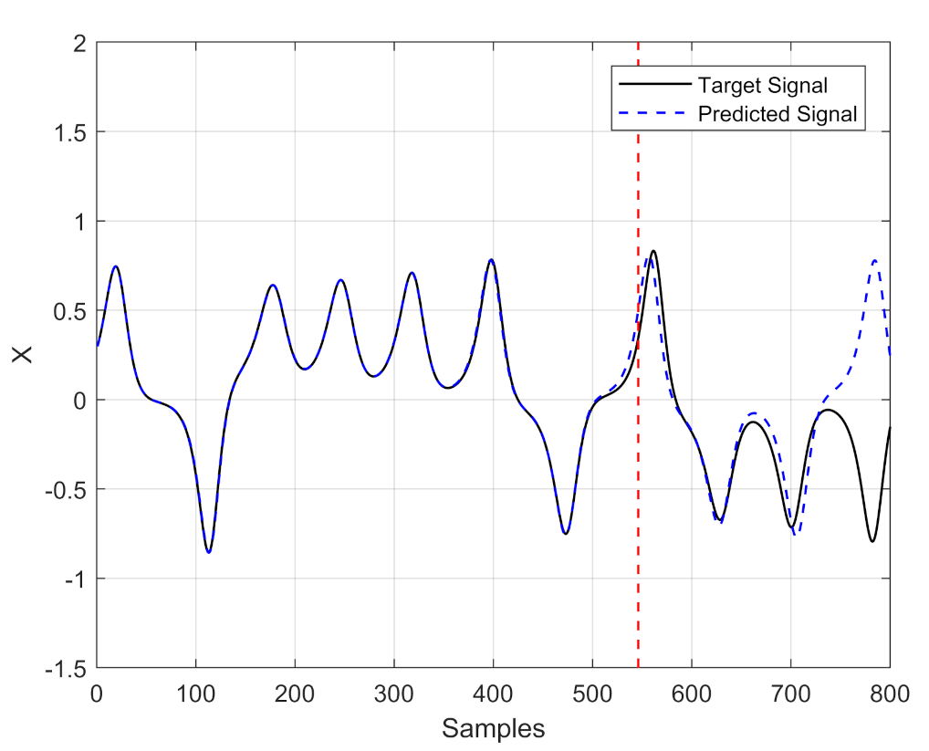
The prediction of chaotic time series is a complex task due to characteristics such as its aperiodic behavior and the high sensitivity to initial conditions. In this manner, the prediction of chaotic time series can be defined as a task where temporal correlations must be learned, this is because the inputs and outputs are ordered sequentially, as shown in Figure 1. That is, they are temporally correlated, and it results that RNNs [38] were developed to learn temporal correlations. Figure 1 sketches the prediction of a chaotic time series, where the red dotted line indicates the forecast horizon reached, and how the predicted time series diverges from the target series.

The main goal in the prediction of chaotic time series is devoted to increasing the prediction window (either by increasing the Lyapunov times or the number of steps ahead) [39,40,41,42]. For instance, the prediction horizon described by (1) can be calculated in the time interval during which the normalized error is less than a threshold k[43,44,45], where $y_{target}$ is associated to the data to predict $y_{}\left(i\right)$, the predicted data, and $HP$, the prediction horizon. In the particular case of applying an ML method based on neural networks as RNN or ESN, the challenges are how to reduce the computational cost, the number of neurons [46], proposing different internal connections [47,48], and how to reduce the prediction error. Usually, the prediction is generally performed to estimate one step ahead or very few steps ahead, and it is sought to have the lowest possible error [49]. In the majority of cases, the prediction error is evaluated as the root mean squared error (RMSE), and it can take different magnitudes to validate the predicted steps ahead.

Table 2. Prediction of chaotic time series using Machine Learning techniques.

ML	Dataset	Steps Ahead	${\mathit{\lambda }}_{max}^{-1}$	RMSE
ESN [50]	Lorenz	300	—	—
ESN [51]	Lorenz	460	10.35	—
RNN-LSTM [51]	Lorenz	180	4.05	—
ANN [51]	Lorenz	120	2.7	—
CEEMDAN-LSTM [52]	Lorenz	—	2	$1.327$
ESN [41]	Lorenz	700	—	—
RESN [39]	Lorenz	500	—	$0.2238$
	Rossler	500	—	$0.1128$
AESN [53]	Lorenz	1	—	$6\times {10}^{-3}$
	Rossler	1	—	$1.65\times {10}^{-2}$
HESN [44]	Lorenz	—	12	—
DPM [54]	Lorenz	300	—	$3.3\times {10}^{-3}$
Fuzzy [55]	Mackey-Glass	1000	—	$3.8\times {10}^{-3}$
ADRC [42]	Rossler	40	—	$1.41\times {10}^{-2}$
ALM-ESN [49]	Lorenz	1	—	$2.21\times {10}^{-5}$
	Mackey-Glass	84	—	$1.9268\times {10}^{-4}$
HESN [40]	Rossler	28	—	$0.8890$
FESN [46]	Mackey-Glass	20	—	—
NARX [56]	Chaotic Serie	600	—	$6.81\times {10}^{-2}$
ESN [56]	Chaotic Serie	600	—	$2.94\times {10}^{-2}$
ESN (This work)	Lorenz	500	—	$5.9095\times {10}^{-2}$

summarizes some relevant works for the prediction of chaotic time series, where ${\lambda }_{max}^{-1}$ represents the Lyapunov times that correspond to the inverse of the maximum Lyapunov exponent of the system. On this issue, it is well known that chaotic behavior can be generated from a mathematical model having at least three ODEs, so that one can evaluate three Lyapunov exponents (one negative, one close to zero and one positive). Systems with more than three ODEs can generate hyperchaos if they have more than one positive Lyapunov exponent. The maximum Lyapunov exponent is then a reference to indicate chaotic behavior and to calculate Lyapunov time, which sometimes is used to measure the prediction window. However, as shown in Table 2, the majority of authors do not report which Lyapunov exponent they use. In the same Table 2, it can be appreciated that the most used chaotic systems are: Lorenz, Rössler and Mackey–Glass, for which the different ML methods predict from 1 to 1000 steps ahead. With respect to the ML method, one can appreciate that ESN and some variants of it have been the most used. For this reason, this paper shows the optimization of an ESN by applying PSO to enhance the prediction horizon.

$$\frac{∥y_{target}\left(i\right)-y_{}\left(i\right)∥}{\sqrt{\frac{1}{HP}{{\sum }_{j=1}^{HP}∥y\left(j\right)∥}^2}}\le k$$

(1)

3. Optimization of ML Methods for Predicting Chaotic Time Series

Generally, when optimizing ML methods to enhance the prediction of chaotic time series, the main focus is to reduce the error in the prediction, so that one can establish the number of steps ahead to be predicted. Let us see some examples: In [57], Lin and Chen optimized a FLNFN (Functional Link-based Neural Fuzzy Network) using a hybrid algorithm consisting of PSO and a cultural algorithm, where the functional expansion in the model can produce the consequent part of a non-linear combination of input variables. The authors used Mackey–Glass time series and forecasted the number of sunspots with the goal of reducing the prediction error by optimizing the fuzzy rules and their relationship with the inputs, but the prediction was only one step ahead. Another work focused on reducing the prediction error by predicting few data is [49], in which a modified version of the Cuckoo Search algorithm was used to optimize a Wavelet Neural Network (WNN) to predict Lorenz time series, showing an improvement of at least $73\%$ over a conventional randomly initialized WNN. Another clear example is given in [58], where Cooperative Coevolution was used to optimize an Elman RNN using time series from Mackey–Glass and Lorenz systems. Other examples are summarized in

Table 3. Optimization algorithms applied to ML methods for the prediction of chaotic time series.

ML	Optimization	Dataset	Fitness Function	Value	Data Test
RVFL [59]	GWO	Oil Layer	Accuracy	$0.91\times {10}^{-1}$	130
	PSO	Oil Layer	Accuracy	$0.92\times {10}^{-1}$	130
	WOA	Oil Layer	Accuracy	$0.85\times {10}^{-1}$	130
FNN [60]	IPBO	Lorenz	MSE	$2.03\times {10}^{-3}$	500
WNN [61]	MCSA	Mackey–Glass	RMSE	$5.60\times {10}^{-5}$	500
		Lorenz	RMSE	$8.20\times {10}^{-3}$	500
LSTM [62]	IHHO	Jinsha River	MAPE$(\%)$	4.19	1753
RNN [63]	NS-ADAM	Electric Power, Nanchang	MSE	$3.26\times {10}^{-3}$	300
CNN-LSTM [64]	GWO	Energy Consumption	MAE	290.5	—

, where one can see optimization algorithms applied to ML methods to predict chaotic time series.

The optimization algorithms given in Table 3 use different error metrics, such as: MSE, RMSE, and MAE described in (2)–(4), respectively [65]. Other recent works, as [66] prefer to introduce a fitness function, such as the one described in (5).

$$MSE=\frac{1}{p}\sum _{i=1}^p{(y_t^i-y^i)}^2$$

(2)

$$RMSE=\sqrt{\frac{1}{p}\sum _{i=1}^p{(y_t^i-y^i)}^2}$$

(3)

$$MAE=\frac{1}{p}\sum _{i=1}^p|y_t-y|$$

(4)

$$fitness\left(FF\right)=Erro{r}_{val}+log(1+8\times Erro{r}_{tst})$$

(5)

4. Optimizing an ESN by PSO to Enhance Time Series Prediction Horizon

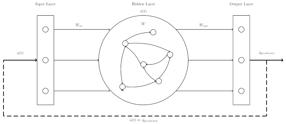
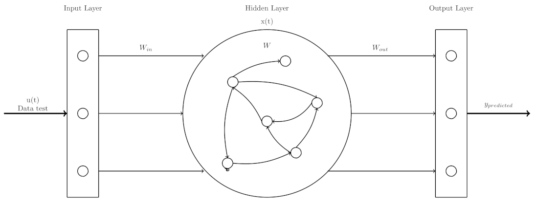
As shown in Table 2, one of the most used ML methods for the prediction of chaotic time series is the Echo State Network (ESN) one. It consists of three layers: the input layer, the hidden layer and the output layer [67]. The hidden layer contains N interconnected neurons with randomly generated weights represented by a matrix $\mathbf{W}.$ESNs have two prediction modes, closed-loop and teacher-forced; in the first mode, the predicted data are used to feedback the network and make the prediction of new data; therefore, a cumulative error is presented, and the predicted data will diverge from the target data; the second makes the prediction of data but it is not used to feedback the ESN, for the prediction of the next data, the point of the test set is taken as input. This implies that only one datum is predicted, and the prediction will not diverge from the target data. Figure 2 shows the closed-loop representation and Figure 3 shows the teacher-forced representation.

Equations (6)–(8) describe the main parameters of the ESN [68], which are mentioned below.

$$\mathbf{x}(\mathbf{t}+\mathbf{1})=(1-a)\mathbf{x}\left(\mathbf{t}\right)+f({\mathbf{W}}_{\mathbf{in}}[b_{in};u(t+1)]+\mathbf{Wx}\left(\mathbf{t}\right))$$

(6)

$$y(t+1)={\mathbf{W}}_{\mathbf{out}}[b_{out};u\left(t\right);\mathbf{x}\left(\mathbf{t}\right)]$$

(7)

$${\mathbf{W}}_{\mathbf{out}}={\mathbf{Y}}^{target}{\mathbf{X}}^T{(\mathbf{X}{\mathbf{X}}^T+\lambda \mathbf{I})}^{-1}$$

(8)

where $\mathbf{x}\left(\mathbf{t}\right)$ represents the states of the neurons, $\mathbf{W}$ is the matrix of internal connections, ${\mathbf{W}}_{\mathbf{in}}$ is the input matrix, ${\mathbf{W}}_{\mathbf{out}}$ is the output matrix, which is interpreted as the trainable parameter, $u\left(t\right)$ is the input, ${\mathbf{Y}}^{target}$ is the data to be learned , $y\left(t\right)$ is the predicted data, and the rest of the parameters are mentioned below.

• Leaking Rate $\left(a\right)$: This parameter is associated with leaky integrator ESNs (LI-ESNs) [69]. These are ESNs whose reservoir neurons perform leaky integration of their activations from past steps of time.
• Spectral Radius (SR): It is described as the maximum absolute eigenvalue of the reservoir weights $\left(\mathbf{W}\right)$. It is recommended that this parameter be between $(0,1)$ to ensure the echo state property [70].
• Reservoir Size (N): The reservoir size N represents the number of neuron units within the reservoir. It is a very crucial parameter, since it decides the maximum number of possible connections within the reservoir $\left(N^2\right)$[71]. Jaeger [71] has suggested that N be in the range $(\frac{T}{10}\le N\le \frac{T}{2})$ with T as the length of training data.
• Input $\left(b_{in}\right)$/Output scaling $\left(b_{out}\right)$: The input weight $\left({\mathbf{W}}_{\mathbf{in}}\right)$ influences the level of the linearity of the responses of reservoir units. For a ${\mathbf{W}}_{\mathbf{in}}$ that is uniformly distributed, the input scaling $b_{in}$ is referred to as a range $[-b;b]$ from which values of ${\mathbf{W}}_{\mathbf{in}}$ are drawn.
• Reservoir Activation Function: For the ESN, the reservoir activation is a non-linear function. In most works, the function of choice has been the $tanh(.)$ or positive logistic $sign(.)$ [72].
• Regularization parameter of ridge regression (RR): Regularization is often aimed at reducing the noise sensitivity of the network and also to prevent overfitting [73].

The case study herein is the prediction of chaotic data from the Lorenz system, whose mathematical model is given in Table 1. To improve the prediction, it is recommended to normalize or scale the amplitudes of the state variables to be within the range of [−1 …1]. For the time series prediction, we use 5000 data for training, an ESN with 500 neurons $\left(\frac{1}{10}T\right)$, $SR=1.25$, $a=0.5$, $RR=1\times {10}^{-8}$, the matrices ${\mathbf{W}}_{\mathbf{in}}$ and $\mathbf{W}$ were randomly generated, and the matrix $\mathbf{W}$ was re-scaled according to the spectral radius.

To optimize the ESN with the parameters described above, we apply PSO, which is inspired from the swarming behavior of certain animals such as fishes and birds. The initial population is generated in a specific space. Each particle p is marked by a pair of position and velocity ($x_i$, $v_i$), and it must be updated according to Equations (9) and (10). Then, the particles swarm flies throughout the search space. Every particle i moves according to its corresponding $v_i$ vector. At each time step, the solutions quality is evaluated according to a fitness function or objective function [74,75]. The general process to optimize an ESN in the chaotic time series prediction task is described below in Algorithm 1. In this case study, we have no constraints.

$$v_{ij}=v_{ij}+c_{1}rand\left(\right)(p_{ij}-x_{ij})+c_{2}rand\left(\right)(g_j-x_{ij})$$

(9)

$$x_{ij}=x_{ij}+v_{ij}$$

(10)

Algorithm 1: Optimization of an ESN to predict the Lorenz system with PSO.

1: Initialize the first particle of the population with known parameters, and the rest randomly $\left(\mathbf{x}\right)$. 2: Initialize the velocity of the particles v. 3: for ($counter=1$; $counter\le G$; $counter++$) do 4:    for ($i=1$; $i\le N_p$; $i++$) do 5:      for ($j=1$; $j\le D$; $j++$) do 6:           For each set of particles (p), train the ESN, re-scaling W matrix according to the corresponding new spectral radius. 7:           Compute $W_{out}$ for each set of (p). 8:           Predict the Lorenz system time series with each set of (p). 9:           Calculate the fitness function, MSE between the predicted and target data. 10:         Find the best value from p and save it in g 11:         Evaluate the new velocity using (9). 12:         Evaluate the new position using (10). 13:      end for 14:      $f_x\leftarrow func\left(x_i\right)$ 15:      if $f_x$ is better than $scor{e}_i$ then 16:         $scor{e}_i\leftarrow f_x$ 17:         $p_i\leftarrow x_i$ 18:         if $p_i$ is better than g then 19:           $g\leftarrow p_i$ 20:         end if 21:      end if 22:    end for 23: end for 24 return  $x,p,g$ and $score$

Although there are general recommendations to select the hyperparameters of the ESN, it is still a design problem; therefore, these parameters must be adjusted according to each problem. For this reason, we decided to optimize the hyperparameters $SR,a,RR$, to find the best values that allow having a lower MSE between the predicted data and the target data. For PSO, we established a population of 30 particles, 10 generations, and 3 variables to optimize in the following ranges: $SR$ = [0.01:1.5], a = [0.01:1], $RR$ = [$1\times {10}^{-10}$:$1\times {10}^{-5}$].

Table 4. ESN optimization using PSO to predict the time series of the Lorenz system.

Parameters	$\mathbf{SR}$	a	$\mathbf{RR}$	MSE	Data Test
Original	1.2500	0.5000	$1\times {10}^{-8}$	$6.4471\times {10}^{-2}$	1000
Solution 1	1.3540	0.5466	$1\times {10}^{-5}$	$1.0569\times {10}^{-4}$	1000
Solution 2	1.3208	0.5811	$1\times {10}^{-5}$	$1.7487\times {10}^{-4}$	1000
Solution 3	1.1338	0.3308	$1\times {10}^{-5}$	$4.5692\times {10}^{-4}$	1000
Solution 4	1.2694	0.4846	$1\times {10}^{-5}$	$2.8641\times {10}^{-4}$	1000
Solution 5	1.3332	0.5690	$1\times {10}^{-5}$	$9.1085\times {10}^{-3}$	1000

shows five solutions in which MSE was reduced with respect to the original parameters.

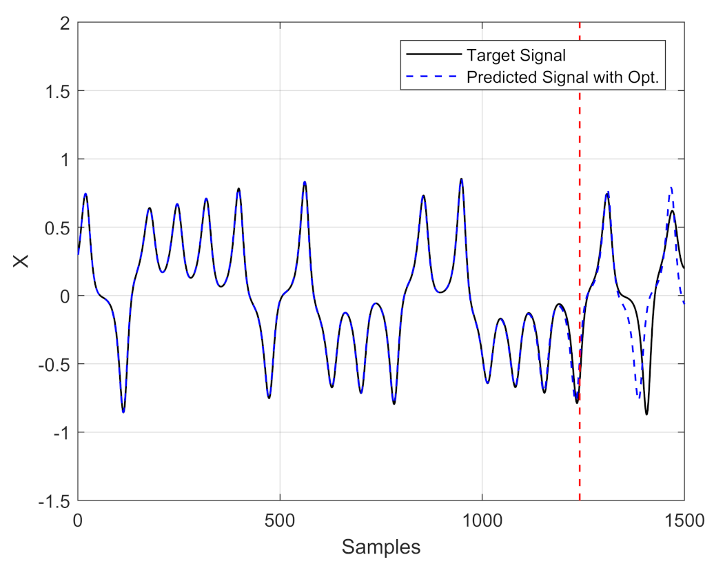
Figure 4 shows the time series prediction of the Lorenz system with the first set of optimized ESN parameters. Compared to the prediction results shown in Figure 1, where the ESN is not optimized, one can see that the prediction horizon doubles, so that there is an increase from 540 to 1240 steps ahead.

5. Discussion

An ESN is a Machine Learning method that has been widely used in the prediction of chaotic time series due to its good results in this task, low computational cost and easy training compared to other recurrent neural networks such as LSTM. However, like many neural networks, they have hyperparameters that must be set before training. In the case of ESNs, the main hyperparameters are the number of neurons, the leaking rate, the spectral radius and the regression coefficient, and although the authors in [70] recommend some ranges of values, there is not an exact way to find them. Starting from the previous premise, the optimization techniques allow finding the set of hyperparameters with which a greater prediction horizon can be obtained. In this manner, we have shown that the use of the PSO algorithm, which is one of the classics in the literature, allows one to optimize the hyperparameters of an ESN in closed-loop mode. This issue also shows that the values of the hyperparameters must be correctly selected to reach a large prediction horizon of chaotic time series. The time series prediction was performed by executing different experiments with different tests, showing that in all of them, the MSE error was reduced, and the prediction was greatly improved with respect to using an ESN without optimization. The different tests provided, on average, an increase in the prediction horizon of a little more than double. As one can infer, there are other optimization algorithms that can be used for the ESN; however, one must be aware that the use of other optimization algorithms does not guarantee that the prediction horizon will increase. The application of an optimization algorithm in this case is just devoted to the search for the ideal combination of hyperparameters, not for improving an ESN topology or its composition, which should imply a much more robust and complex design problem.

In the state of the art, one can find several optimization algorithms that have been applied to optimize an ESN to predict chaotic time series. For instance,

Table 5. Optimization algorithms applied to an ESN to predict chaotic time series.

Optimization	Dataset	Fitness Function	Value	Data Test
BSA [76]	Canadan Lynx	MSE	$5.17\times {10}^{-2}$	14
PSO [65]	Lorenz	RMSE	$2.01\times {10}^{-3}$	500
	Mackey–Glass	RMSE	$2.97\times {10}^{-3}$	500
CS [77]	Mackey–Glass	MSE	$8.74\times {10}^{-9}$	1000
FOA [78]	Lorenz	RMSE	$8.20\times {10}^{-3}$	4000
	Mackey–Glass	RMSE	$9.60\times {10}^{-3}$	1000
SOGWO [79]	Mackey–Glass	RMSE	$1.46\times {10}^{-4}$	800
WOA [66]	Lorenz	FF	$7.37\times {10}^{-8}$	600
GA [66]	Lorenz	FF	$5.54\times {10}^{-6}$	600
PSO [80]	Lorenz	RMSE	$3.24\times {10}^{-2}$	500
BGWO [81]	Mackey–Glass	RMSE	$1.03\times {10}^{-2}$	500
DE [82]	Mackey–Glass	NRMSE	$2.59\times {10}^{-4}$	2000
PSO [83]	Mackey–Glass	MSE	$8.12\times {10}^{-5}$	1000
Neuro-Evolution [84]	Hénon	NMSE	$4.23\times {10}^{-3}$	3000
MBBO [85]	Lorenz	RMSE	$2.28\times {10}^{-4}$	2000
PSO (This work)	Lorenz	MSE	$1.0569\times {10}^{-4}$	1000

shows different evolutionary algorithms, and among them, one can see the application of PSO to optimize the ESN using different error values for the fitness functions and for different lengths of the data test. In such a table, one can see our results compared to published works, so that for chaotic time series of the Lorenz system, we reach the lowest error using 1000 data. It may be difficult to perform a comparison between the results obtained in our experiments and the results reported in the literature. This is because there are two types of prediction that can be made with an ESN: the closed-loop and teacher-forced. In the first mode, the predicted data are used to feedback the network, which causes the errors to accumulate and eventually diverges the predicted data from the target data. In the second, or teacher-forced mode, the predicted data are not fed back to the ESN, but the input comes directly from the data of the test set, which implies that only one datum is predicted. From Table 5, one can see the size of the data test for each case, but the authors do not mention what type of prediction they make. For example, in [66], Zhang et al. report a very small error in the time series prediction, but they do not specify what type of prediction is performed. The prediction mode is quite important, since using teacher-forced, there is not a cumulative error problem and generally the prediction will not diverge from the target data. In this manner, our contribution relies on the use of the closed-loop prediction mode, since the main goal of this work was focused on increasing the prediction horizon for chaotic time series, and this has been performed with the help of an optimization algorithm, i.e., PSO, to accomplish the correct selection of the hyperparameters of an ESN.

6. Conclusions

Although a great variety of ML methods have been used for the prediction of chaotic time series, this work showed that ESN is one of the most used. The optimization of ML methods, as those based on neural networks such as ESN, focus on finding the best values of the hyperparameters that minimize the prediction error. However, it is necessary to determine which parameters should be optimized for each problem. It should also be considered that EAs are metaheuristics, and they have their own parameters that must be carefully selected, such as the size of the population and the number of generations, among others. Another consideration is the fitness function that is chosen. Generally, some measure of error between the predicted values and the target values is used, but a good alternative would be to use measures such as maximizing the prediction horizon. Finally, it is worthwhile to mention a very interesting aspect when optimizing an ESN for the prediction of chaotic time series: the type of prediction that is made, which can be in closed-loop or teacher-forced mode. The first mode should be used when seeking to increase the prediction horizon, and the second can be used when the goal is to reduce the error in the prediction; however, usually, this is not specified in the works. To verify the importance of the selection of hyperparameters in a machine learning method for forecasting chaotic time series, we used PSO to optimize a closed-loop ESN, which allowed us to increase the forecast horizon around the double compared to a non-optimized ESN.

References

- Nadiga, B.T. Reservoir Computing as a Tool for Climate Predictability Studies. J. Adv. Model. Earth Syst. 2021, 13, e2020MS002290. [Google Scholar] [CrossRef]
- Dueben, P.D.; Bauer, P. Challenges and design choices for global weather and climate models based on machine learning. Geosci. Model Dev. 2018, 11, 3999–4009. Available online: https://gmd.copernicus.org/articles/11/3999/2018/ (accessed on 31 August 2022). [CrossRef] [Green Version]
- Scher, S. Toward Data-Driven Weather and Climate Forecasting: Approximating a Simple General Circulation Model With Deep Learning. Geophys. Res. Lett. 2018, 12, 12616–12622. [Google Scholar] [CrossRef] [Green Version]
- Bec, J.; Biferale, L.; Boffetta, G.; Cencini, M.; Musacchio, S.; Toschi, F. Lyapunov exponents of heavy particles in turbulence. Phys. Fluids 2006, 18, 091702. [Google Scholar] [CrossRef] [Green Version]
- Hassanaly, M.; Raman, V. Ensemble-LES analysis of perturbation response of turbulent partially-premixed flames. Proc. Combust. Inst. 2019, 37, 2249–2257. Available online: https://www.sciencedirect.com/science/article/pii/S154074891830395X (accessed on 31 August 2022). [CrossRef] [Green Version]
- Nastac, G.; Labahn, J.W.; Magri, L.; Ihme, M. Lyapunov exponent as a metric for assessing the dynamic content and predictability of large-eddy simulations. Phys. Rev. Fluids 2017, 2, 094606. [Google Scholar] [CrossRef]
- Shahi, S.; Marcotte, C.D.; Herndon, C.J.; Fenton, F.H.; Shiferaw, Y.; Cherry, E.M. Long-Time Prediction of Arrhythmic Cardiac Action Potentials Using Recurrent Neural Networks and Reservoir Computing. Front. Physiol.202112734178. Available online: https://www.ncbi.nlm.nih.gov/pmc/articles/PMC8502981/ (accessed on 31 August 2022).
- Pathak, J.; Hunt, B.; Girvan, M.; Lu, Z.; Ott, E. Model-Free Prediction of Large Spatiotemporally Chaotic Systems from Data: A Reservoir Computing Approach. Phys. Rev. Lett. 2018, 120, 024102. [Google Scholar] [CrossRef] [Green Version]
- Hüsken, M.; Stagge, P. Recurrent neural networks for time series classification. Neurocomputing 2003, 50, 223–235. Available online: https://www.sciencedirect.com/science/article/pii/S0925231201007068 (accessed on 31 August 2022). [CrossRef]
- Lin, X.; Yang, Z.; Song, Y. Short-term stock price prediction based on echo state networks. Expert Syst. Appl. 2009, 36, 7313–7317. Available online: https://www.sciencedirect.com/science/article/pii/S0957417408006519 (accessed on 31 August 2022). [CrossRef]
- Yao, K.; Huang, K.; Zhang, R.; Hussain, A. Improving Deep Neural Network Performance with Kernelized Min-Max Objective. In Neural Information Processing; Series Lecture Notes in Computer Science; Cheng, L., Leung, A., Ozawa, S., Eds.; Springer International Publishing: Cham, Switzerland, 2018; pp. 182–191. [Google Scholar]
- Han, M.; Xu, M. Laplacian Echo State Network for Multivariate Time Series Prediction. IEEE Trans. Neural Netw. Learn. Syst. 2018, 29, 238–244. [Google Scholar] [CrossRef]
- Wikner, A.; Pathak, J.; Hunt, B.; Girvan, M.; Arcomano, T.; Szunyogh, I.; Pomerance, A.; Ott, E. Combining machine learning with knowledge-based modeling for scalable forecasting and subgrid-scale closure of large, complex, spatiotemporal systems. Chaos Interdiscip. J. Nonlinear Sci. 2020, 30, 053111. [Google Scholar] [CrossRef] [PubMed]
- Sheng, C.; Zhao, J.; Wang, W.; Leung, H. Prediction intervals for a noisy nonlinear time series based on a bootstrapping reservoir computing network ensemble. IEEE Trans. Neural Netw. Learn. Syst. 2013, 24, 1036–1048. [Google Scholar] [CrossRef] [PubMed]
- Yang, C.; Qiao, J.; Han, H.; Wang, L. Design of polynomial echo state networks for time series prediction. Neurocomputing 2018, 290, 148–160. Available online: https://www.sciencedirect.com/science/article/pii/S0925231218301711 (accessed on 31 August 2022). [CrossRef]
- Malik, Z.; Hussain, A.; Wu, Q. Multilayered Echo State Machine: A Novel Architecture and Algorithm. IEEE Trans. Cybern. 2017, 47, 946–959. [Google Scholar] [CrossRef] [Green Version]
- Schäfer, A.; Zimmermann, H.-G. Recurrent neural networks are universal approximators. Int. J. Neural Syst. 2007, 17, 253–263. [Google Scholar] [CrossRef]
- Siegelmann, H.T.; Sontag, E.D. Turing computability with neural nets. Appl. Math. Lett. 1991, 4, 77–80. Available online: https://www.sciencedirect.com/science/article/pii/089396599190080F (accessed on 31 August 2022). [CrossRef] [Green Version]
- Jaeger, H. The “echo state” approach to analysing and training recurrent neural networks-with an erratum note. Bonn Ger. Ger. Natl. Res. Cent. Inf. Technol. GMD Tech. Rep. 2001, 148, 13. [Google Scholar]
- Shen, L.; Chen, J.; Zeng, Z.; Yang, J.; Jin, J. A novel echo state network for multivariate and nonlinear time series prediction. Appl. Soft Comput. 2018, 62, 524–535. Available online: https://www.sciencedirect.com/science/article/pii/S1568494617306439 (accessed on 31 August 2022). [CrossRef]
- Maass, W.; Natschläger, T.; Markram, H. Real-Time Computing Without Stable States: A New Framework for Neural Computation Based on Perturbations. Neural Comput. 2002, 14, 2531–2560. [Google Scholar] [CrossRef]
- Yperman, J.; Becker, T. Bayesian optimization of hyper-parameters in reservoir computing. arXiv 2016, arXiv:1611.05193. [Google Scholar]
- Zhang, C.; Lin, Q.; Gao, L.; Li, X. Backtracking Search Algorithm with three constraint handling methods for constrained optimization problems. Expert Syst. Appl. 2015, 42, 7831–7845. Available online: https://www.sciencedirect.com/science/article/pii/S0957417415003863 (accessed on 31 August 2022). [CrossRef]
- Dorigo, M. Optimization, Learning and Natural Algorithms. Ph.D. Thesis, Politecnico di Milano, Milan, Italy, 1992. [Google Scholar]
- Yang, X.-S. Nature-Inspired Metaheuristic Algorithms; Luniver Press: 2010. Available online: www.luniver.com (accessed on 31 August 2022).
- Yang, X.-S.; Deb, S. Cuckoo Search via Lévy flights. In Proceedings of the 2009 World Congress on Nature & Biologically Inspired Computing (NaBIC), Coimbatore, India, 9–11 December 2009; pp. 210–214. [Google Scholar]
- Kennedy, J.; Eberhart, R. Particle swarm optimization. In Proceedings of theICNN’95—International Conference on Neural Networks, Perth, WA, Australia, 27 November–1 December 1995; Volume 4, pp. 1942–1948. [Google Scholar]
- Strogatz, S. Nonlinear Dynamics and Chaos (Studies in Nonlinearity); Westview Press: Boulder, CO, USA, 1994. [Google Scholar]
- Lorenz, E.N. Deterministic Nonperiodic Flow. J. Atmos. Sci. 1963, 20, 130–141. Available online: https://journals.ametsoc.org/view/journals/atsc/20/2/1520-0469-1963-020-0130-dnf-2-0-co-2.xml (accessed on 31 August 2022). [CrossRef]
- Rössler, O.E. An equation for continuous chaos. Phys. Lett. A 1976, 57, 397–398. Available online: https://www.sciencedirect.com/science/article/pii/0375960176901018 (accessed on 31 August 2022). [CrossRef]
- Leonov, G.A.; Kuznetsov, N.V. On differences and similarities in the analysis of Lorenz, Chen, and Lu systems. Appl. Math. Comput. 2015, 256, 334–343. Available online: http://www.sciencedirect.com/science/article/pii/S0096300314017937 (accessed on 31 August 2022). [CrossRef] [Green Version]
- Augustová, P.; Beran, Z. Characteristics of the Chen Attractor. In Nostradamus 2013: Prediction, Modeling and Analysis of Complex Systems; Series Advances in Intelligent Systems and Computing; Zelinka, I., Chen, G., Rössler, O., Snasel, V., Abraham, A., Eds.; Springer International Publishing: Berlin/Heidelberg, Germany, 2013; Volume 210, pp. 305–312. [Google Scholar]
- Zhong, G.-Q.; Ayrom, F. Experimental confirmation of chaos from Chua’s circuit. Int. J. Circuit Theory Appl. 1985, 13, 93–98. [Google Scholar] [CrossRef]
- Tsaneva-Atanasova, K.; Osinga, H.M.; Rieß, T.; Sherman, A. Full system bifurcation analysis of endocrine bursting models. J. Theor. Biol. 2010, 264, 1133–1146. Available online: https://www.sciencedirect.com/science/article/pii/S0022519310001633 (accessed on 31 August 2022). [CrossRef] [Green Version]
- González-Zapata, A.M.; Tlelo-Cuautle, E.; Cruz-Vega, I.; León-Salas, W.D. Synchronization of chaotic artificial neurons and its application to secure image transmission under MQTT for IoT protocol. Nonlinear Dyn. 2021, 104, 4581–4600. [Google Scholar] [CrossRef]
- Tlelo-Cuautle, E.; González-Zapata, A.M.; Díaz-Muñoz, J.D.; Fraga, L.G.d.; Cruz-Vega, I. Optimization of fractional-order chaotic cellular neural networks by metaheuristics. Eur. Phys. J. Spec. Top. 2022, 231, 2037–2043. [Google Scholar] [CrossRef]
- Tlelo-Cuautle, E.; Díaz-Muñoz, J.D.; González-Zapata, A.M.; Li, R.; León-Salas, W.D.; Fernández, F.V.; Guillén-Fernández, O.; Cruz-Vega, I. Chaotic Image Encryption Using Hopfield and Hindmarsh–Rose Neurons Implemented on FPGA. Sensors 2020, 20, 1326. [Google Scholar] [CrossRef] [Green Version]
- Rumelhart, D.E.; Hinton, G.E.; Williams, R.J. Learning representations by back-propagating errors. Nature 1986, 323, 533–536. Available online: https://www.nature.com/articles/323533a0 (accessed on 31 August 2022). [CrossRef]
- Li, D.; Han, M.; Wang, J. Chaotic Time Series Prediction Based on a Novel Robust Echo State Network. IEEE Trans. Neural Netw. Learn. Syst. 2012, 23, 787–799. [Google Scholar] [CrossRef] [PubMed]
- Xu, M.; Han, M.; Qiu, T.; Lin, H. Hybrid Regularized Echo State Network for Multivariate Chaotic Time Series Prediction. IEEE Trans. Cybern. 2019, 49, 2305–2315. [Google Scholar] [CrossRef] [PubMed]
- Bompas, S.; Georgeot, B.; Guéry-Odelin, D. Accuracy of neural networks for the simulation of chaotic dynamics: Precision of training data vs precision of the algorithm. Chaos Interdiscip. J. Nonlinear Sci. 2020, 30, 113118. [Google Scholar] [CrossRef]
- Bo, Y.-C.; Wang, P.; Zhang, X. An asynchronously deep reservoir computing for predicting chaotic time series. Appl. Soft Comput. 2020, 95, 106530. Available online: https://www.sciencedirect.com/science/article/pii/S1568494620304695 (accessed on 31 August 2022). [CrossRef]
- Doan, N.A.K.; Polifke, W.; Magri, L. Physics-Informed Echo State Networks for Chaotic Systems Forecasting. In Computational Science—ICCS 2019; Series Lecture Notes in Computer Science; Rodrigues, J.M.F., Cardoso, P.J.S., Monteiro, J., Lam, R., Krzhizhanovskaya, V.V., Lees, M.H., Dongarra, J.J., Sloot, P.M., Eds.; Springer International Publishing: Cham, Switzerland, 2019; pp. 192–198. [Google Scholar]
- Pathak, J.; Wikner, A.; Fussell, R.; Chandra, S.; Hunt, B.R.; Girvan, M.; Ott, E. Hybrid forecasting of chaotic processes: Using machine learning in conjunction with a knowledge-based model. Chaos Interdiscip. J. Nonlinear Sci. 2018, 28, 041101. [Google Scholar] [CrossRef] [PubMed] [Green Version]
- Racca, A.; Magri, L. Robust Optimization and Validation of Echo State Networks for learning chaotic dynamics. Neural Netw. 2021, 142, 252–268. Available online: https://www.sciencedirect.com/science/article/pii/S0893608021001969 (accessed on 31 August 2022). [CrossRef]
- Yao, X.; Wang, Z. Fractional Order Echo State Network for Time Series Prediction. Neural Process. Lett. 2020, 52, 603–614. [Google Scholar] [CrossRef]
- Hua, Y.; Zhao, Z.; Li, R.; Chen, X.; Liu, Z.; Zhang, H. Deep Learning with Long Short-Term Memory for Time Series Prediction. IEEE Commun. Mag. 2019, 57, 114–119. [Google Scholar] [CrossRef] [Green Version]
- Griffith, A.; Pomerance, A.; Gauthier, D.J. Forecasting chaotic systems with very low connectivity reservoir computers. Chaos Interdiscip. J. Nonlinear Sci. 2019, 29, 123108. [Google Scholar] [CrossRef] [Green Version]
- Qiao, J.; Wang, L.; Yang, C.; Gu, K. Adaptive Levenberg-Marquardt Algorithm Based Echo State Network for Chaotic Time Series Prediction. IEEE Access 2018, 6, 10720–10732. [Google Scholar] [CrossRef]
- Pathak, J.; Lu, Z.; Hunt, B.R.; Girvan, M.; Ott, E. Using machine learning to replicate chaotic attractors and calculate Lyapunov exponents from data. Chaos Interdiscip. J. Nonlinear Sci. 2017, 27, 121102. [Google Scholar] [CrossRef] [PubMed]
- Chattopadhyay, A.; Hassanzadeh, P.; Subramanian, D. Data-driven predictions of a multiscale Lorenz 96 chaotic system using machine-learning methods: Reservoir computing, artificial neural network, and long short-term memory network. Nonlinear Process. Geophys. 2020, 27, 373–389. Available online: https://npg.copernicus.org/articles/27/373/2020/ (accessed on 31 August 2022). [CrossRef]
- Yanan, G.; Xiaoqun, C.; Bainian, L.; Kecheng, P. Chaotic Time Series Prediction Using LSTM with CEEMDAN. J. Phys. Conf. Ser. 2020, 1617, 012094. [Google Scholar] [CrossRef]
- Xu, M.; Han, M. Adaptive Elastic Echo State Network for Multivariate Time Series Prediction. IEEE Trans. Cybern. 2016, 46, 2173–2183. [Google Scholar] [CrossRef] [PubMed]
- Guo, X.; Sun, Y.; Ren, J. Low dimensional mid-term chaotic time series prediction by delay parameterized method. Inf. Sci. 2020, 516, 1–19. Available online: https://www.sciencedirect.com/science/article/pii/S0020025519311351 (accessed on 31 August 2022). [CrossRef]
- Alemu, M.N. A Fuzzy Model for Chaotic Time Series Prediction. Int. J. Innov. Comput. Inf. Control. 2018, 14, 1767–1786. [Google Scholar] [CrossRef]
- Pano-Azucena, A.D.; Tlelo-Cuautle, E.; Ovilla-Martinez, B.; Fraga, L.G.d.; Li, R. Pipeline FPGA-Based Implementations of ANNs for the Prediction of up to 600-Steps-Ahead of Chaotic Time Series. J. Circuits Syst. Comput. 2021, 30, 2150164. [Google Scholar] [CrossRef]
- Lin, C.-J.; Chen, C.-H.; Lin, C.-T. A Hybrid of Cooperative Particle Swarm Optimization and Cultural Algorithm for Neural Fuzzy Networks and Its Prediction Applications. IEEE Trans. Syst. Man Cybern. Part C (Appl. Rev.) 2009, 39, 55–68. [Google Scholar]
- Chandra, R. Competition and Collaboration in Cooperative Coevolution of Elman Recurrent Neural Networks for Time-Series Prediction. IEEE Trans. Neural Netw. Learn. Syst. 2015, 26, 3123–3136. [Google Scholar] [CrossRef] [Green Version]
- Lan, P.; Xia, K.; Pan, Y.; Fan, S. An Improved GWO Algorithm Optimized RVFL Model for Oil Layer Prediction. Electronics 2021, 10, 3178. [Google Scholar] [CrossRef]
- Cao, Z. Evolutionary optimization of artificial neural network using an interactive phase-based optimization algorithm for chaotic time series prediction. Soft Comput. 2020, 24, 17093–17109. [Google Scholar] [CrossRef]
- Ong, P.; Zainuddin, Z. Optimizing wavelet neural networks using modified cuckoo search for multi-step ahead chaotic time series prediction. Appl. Soft Comput. 2019, 80, 374–386. Available online: https://www.sciencedirect.com/science/article/pii/S1568494619302078 (accessed on 31 August 2022). [CrossRef]
- Sun, W.; Peng, T.; Luo, Y.; Zhang, C.; Hua, L.; Ji, C.; Ma, H. Hybrid short-term runoff prediction model based on optimal variational mode decomposition, improved Harris hawks algorithm and long short-term memory network. Environ. Res. Commun. 2022, 4, 045001. [Google Scholar] [CrossRef]
- Zhang, Y.; Wang, Y.; Luo, G. A new optimization algorithm for non-stationary time series prediction based on recurrent neural networks. Future Gener. Comput. Syst. 2020, 102, 738–745. Available online: https://www.sciencedirect.com/science/article/pii/S0167739X18332540 (accessed on 31 August 2022). [CrossRef]
- Xie, H.; Zhang, L.; Lim, C.P. Evolving CNN-LSTM Models for Time Series Prediction Using Enhanced Grey Wolf Optimizer. IEEE Access 2020, 8, 161519–161541. [Google Scholar] [CrossRef]
- Chouikhi, N.; Ammar, B.; Rokbani, N.; Alimi, A.M. PSO-based analysis of Echo State Network parameters for time series forecasting. Appl. Soft Comput. 2017, 55, 211–225. Available online: https://www.sciencedirect.com/science/article/pii/S1568494617300649 (accessed on 31 August 2022). [CrossRef]
- Zhang, M.; Wang, B.; Zhou, Y.; Sun, H. WOA-Based Echo State Network for Chaotic Time Series Prediction. J. Korean Phys. Soc. 2020, 76, 384–391. [Google Scholar] [CrossRef]
- Bala, A.; Ismail, I.; Ibrahim, R.; Sait, S.M. Applications of Metaheuristics in Reservoir Computing Techniques: A Review. IEEE Access 2018, 6, 58012–58029. [Google Scholar] [CrossRef]
- Lukoševičius, M.; Jaeger, H. Reservoir computing approaches to recurrent neural network training. Comput. Sci. Rev. 2009, 3, 127–149. Available online: https://www.sciencedirect.com/science/article/pii/S1574013709000173 (accessed on 31 August 2022). [CrossRef]
- Jaeger, H.; Lukoševičius, M.; Popovici, D.; Siewert, U. Optimization and applications of echo state networks with leaky- integrator neurons. Neural Netw. 2007, 20, 335–352. Available online: https://www.sciencedirect.com/science/article/pii/S089360800700041X (accessed on 31 August 2022). [CrossRef]
- Lukosevicius, M. A Practical Guide to Applying Echo State Networks. In Neural Networks: Tricks of the Trade, 2nd ed.; Montavon, G., Orr, G.B., Müller, K.R., Eds.; Springer: Berlin/Heidelberg, Germany, 2012; pp. 659–686. [Google Scholar] [CrossRef]
- Jaeger, H. Tutorial on Training Recurrent Neural Networks, Covering BPPT, RTRL, EKF and the “Echo State Network” Approach; GMD-Forschungszentrum Informationstechnik: Bonn, Germany, 2002; Volume 5. [Google Scholar]
- Wang, S.; Yang, X.-J.; Wei, C.-J. Harnessing Non-linearity by Sigmoid-wavelet Hybrid Echo State Networks (SWHESN). In Proceedings of the 2006 6th World Congress on Intelligent Control and Automation, Dalian, China, 21–23 June 2006; Volume 1, pp. 3014–3018. [Google Scholar]
- Verducci, J.S. Prediction and Discovery: AMS-IMS-SIAM Joint Summer Research Conference, Machine and Statistical Learning: Prediction and Discovery, June 25–29, 2006, Snowbird, Utah; American Mathematical Society: Providence, RI, USA, 2007. [Google Scholar]
- Shi, Y. Particle Swarm Optimization. IEEE Connect. 2014, 2, 8–13. Available online: https://www.marksmannet.com/RobertMarks/Classes/ENGR5358/Papers/pso_bySHI.pdf (accessed on 31 August 2022).
- Bai, Q. Analysis of particle swarm optimization algorithm. Comput. Inf. Sci. 2010, 3, 180. [Google Scholar] [CrossRef] [Green Version]
- Wang, Z.; Zeng, Y.-R.; Wang, S.; Wang, L. Optimizing echo state network with backtracking search optimization algorithm for time series forecasting. Eng. Appl. Artif. Intell. 2019, 81, 117–132. Available online: https://www.sciencedirect.com/science/article/pii/S0952197619300326 (accessed on 31 August 2022). [CrossRef]
- Bala, A.; Ismail, I.; Ibrahim, R. Cuckoo Search Based Optimization of Echo State Network for Time Series Prediction. In Proceedings of the 2018 International Conference on Intelligent and Advanced System (ICIAS), Kuala Lumpur, Malaysia, 13–14 August 2018; pp. 1–6. [Google Scholar]
- Tian, Z. Echo state network based on improved fruit fly optimization algorithm for chaotic time series prediction. J. Ambient. Intell. Humaniz. Comput. 2020, 13, 3483–3502. [Google Scholar] [CrossRef]
- Chen, H.-C.; Wei, D.-Q. Chaotic time series prediction using echo state network based on selective opposition grey wolf optimizer. Nonlinear Dyn. 2021, 104, 3925–3935. [Google Scholar] [CrossRef]
- Chouikhi, N.; Fdhila, R.; Ammar, B.; Rokbani, N.; Alimi, A.M. Single- and multi-objective particle swarm optimization of reservoir structure in Echo State Network. In Proceedings of the 2016 International Joint Conference on Neural Networks (IJCNN), Vancouver, BC, Canada, 24–29 July 2016; pp. 440–447. [Google Scholar]
- Liu, J.; Sun, T.; Luo, Y.; Yang, S.; Cao, Y.; Zhai, J. Echo state network optimization using binary grey wolf algorithm. Neurocomputing 2020, 385, 310–318. Available online: https://www.sciencedirect.com/science/article/pii/S0925231219317783 (accessed on 31 August 2022). [CrossRef]
- Yang, C.; Qiao, J.; Wang, L. A novel echo state network design method based on differential evolution algorithm. In Proceedings of the 2017 36th Chinese Control Conference (CCC), Dalian, China, 26–28 July 2017; pp. 3977–3982. [Google Scholar]
- Chouikhi, N.; Ammar, B.; Rokbani, N.; Alimi, A.M.; Abraham, A. A Hybrid Approach Based on Particle Swarm Optimization for Echo State Network Initialization. In Proceedings of the 2015 IEEE International Conference on Systems, Man, and Cybernetics, Hong Kong, China, 9–12 October 2015; pp. 2896–2901. [Google Scholar]
- Otte, S.; Butz, M.V.; Koryakin, D.; Becker, F.; Liwicki, M.; Zell, A. Optimizing recurrent reservoirs with neuro-evolution. Neurocomputing 2016, 192, 128–138. Available online: https://www.sciencedirect.com/science/article/pii/S0925231216002629 (accessed on 31 August 2022). [CrossRef]
- Na, X.; Han, M.; Ren, W.; Zhong, K. Modified BBO-Based Multivariate Time-Series Prediction System With Feature Subset Selection and Model Parameter Optimization. IEEE Trans. Cybern. 2020, 52, 2163–2173. [Google Scholar] [CrossRef]
Figure 1.
Predicting time series of the chaotic Lorenz system using ESN.
Figure 2.
ESN closed-loop.
Figure 3.
ESN teacher-forced.
Figure 4.
Predicting time series of Lorenz system with an optimized ESN.