Article

Multi-Period Spare Parts Supply Chain Network Optimization under (T, s, S) Inventory Control Policy with Improved Dynamic Particle Swarm Optimization

Shijiazhuang Campus, Army Engineering University, Shijiazhuang 050003, China
*
Author to whom correspondence should be addressed.
Electronics 2022, 11(21), 3454; https://doi.org/10.3390/electronics11213454
Submission received: 25 September 2022 / Revised: 12 October 2022 / Accepted: 16 October 2022 / Published: 25 October 2022

Abstract

:

Highlights

What are the main findings?
  • An extended (T, s, S) inventory control strategy is utilized to manage spare parts in customer nodes;
  • A dynamic nonlinear programming model is developed for optimizing inventory control decisions and spare part supply decisions;
  • An improved self-adaptive dynamic migrating PSO is proposed in which a novel environment change detection and response strategy is applied.
What are the implications of the main findings?
  • Solving the joint optimization problem of spare part management and spare part supply chain network optimization under multiple supply periods;
  • The improved dynamic particle swarm optimization algorithm has better computation efficiency and performance than the traditional algorithm.

Abstract

Spare parts are the critical operation asset for ensuring a production line keeps going, which significantly improves the performance of manufacturing enterprises. This article pays attention to the joint optimization of spare part management and spare part supply chain network optimization in multiple supply periods. An extended (T, s, S) inventory control strategy is utilized to manage spare parts in customer nodes which can determine supply time, consumption and demand. In this spare part supply chain, the supply environment is different in different periods, so the mathematical model and solution method should be able to respond to and detect the environment change quickly. Hence, a dynamic nonlinear programming model is developed for optimizing inventory control decisions and spare part supply decisions so as to minimize the total cost. Furthermore, an improved self-adaptive dynamic migrating particle swarm optimization algorithm is proposed to solve the optimization problem. In this algorithm, a novel environment change detection and response strategy is applied to deal with the dynamic period in the spare part supply chain network. The results obtained show that the improved algorithm improves the computation time by eight percent and has better computational efficiency compared with the traditional algorithm.

1. Introduction

Spare parts (SPs) are a critical operational issue for improving equipment reliability, reducing production interruptions as well as enhancing the performance of manufacturing enterprises. The spare part revenue of Germany Dockomo Heavy Machinery Equipment Ltd. reached USD 370 million in 2010 [1]. Spare part management (SPM) has become an important way to improve an enterprise’s economic profit and customer loyalty. Compared with machinery equipment, spare parts are specific products and operational assets, which is reflected in their common function and management characteristics [2]. Natural degradation and random failures, such as gear wear and broken teeth, are the key obstacles to equipment reliability and enterprise performance. Equipment failure without available spare parts will cause a large loss, and a delayed product supply will reduce customer loyalty.
Spare part management consists of all decisions and planning related to spare parts from spare part ordering to storage, classification, inventory management, logistics, and other issues [3,4]. The spare part supply chain includes spare part inventory control and spare part logistics. Although spare part management has a significant positive influence on enterprise performance, the spare part supply chain is ignored or considered a given network in most of the research relating to spare part management [3]. Most of the researchers distinguished between inventory management and the supply chain [5,6,7,8]. However, the spare part supply chain network supports the total SP-related issues, including inventory, order, distribution, transportation, and delivery, which significantly affect the efficiency of spare part management and the performance of the enterprise [9,10]. The joint optimization of spare part supply, inventory, and repair is an emerging area [10]. Thus, this research aims to integrate inventory control and network decisions involving spare part supply chain networks. The proposed joint optimization is developed on the basis of a generic three-echelon spare part supply chain network and inventory control strategy while aiming to minimize the total economic cost, consisting of the spare part ordering cost, transportation cost, inventory holding cost, and equipment breakdown loss.
A change in a spare part’s inventory level is caused by equipment maintenance demand. Replacement maintenance is considered in this paper because this maintenance mode involves replacing components and generates spare part demand. Most of the research focusing on spare part supply considers the demand as a fixed quantity which is disengaged from equipment maintenance activities [11,12]. In this paper, the spare part demand is caused by random equipment failure, which is subject to a common fixed distribution such as the Weibull distribution or exponential distribution.
Another important issue in supply chain optimization is the model solution. The proposed mathematical model is a dynamic nonlinear programming problem, which is difficult to find an appropriate method to solve [13]. The intelligent optimization algorithm has been proven to be an effective method for addressing nonlinear programming problems and other difficult optimization problems [14]. The typical heuristic algorithms are the genetic algorithm (GA), ant colony algorithm (ACO), bat algorithm (BA), and so on. However, the traditional algorithms are applied only to solve static optimization problems and not the dynamic optimization problems in this paper. Therefore algorithms such as particle swarm optimization (PSO) have problems with local convergence and a slow convergence speed. Hence, improved self-adaptive dynamic migrating PSO (SDMPSO) is proposed in this paper. On the basis of the framework of the traditional PSO, the improved SDMPSO can detect the change in the optimization environment and response through the operating population. Moreover, the self-adaptive inertia weight can efficiently improve the convergence performance compared with traditional PSO. Finally, SDMPSO adopts a self-adaptive migrating strategy to seek an excellent trade-off between local exploitation and global exploration of the proposed algorithm.
The construct of this paper is as follows. Section 2 represents the overview of some of the literature involving spare part management, joint optimization of supply and inventory, and model solution. Section 3 develops a multi-period, multi-echelon spare part supply chain network optimization model under the (T, s, S) inventory control policy. The proposed improved SDMPSO algorithm is developed in Section 4. Section 5 represents a numerical example. Some analyses of the results and sensitivity analyses are also conducted in Section 5. Finally, Section 6 presents the conclusions of this research.

2. Literature Review

2.1. Spare Part Management

Most of the literature involving spare part management has been carried out to optimize inventory control strategies. There are various inventory policies that are utilized to apply for various spare parts. Based on different reviewing methods, the inventory policies can be divided into continuous review policies and periodic review policies. According to the size of the spare part replenishment order, the policies can be divided into fixed quantity and variable quantity orders. Hence, on the basis of the aforementioned classification standards, each current inventory can be defined and classified clearly. The (T, Q) policy considers a periodic review with a fixed replenishment order size [15]. The (T, S) policy replenishes a variable number of spare parts under a periodic review [11]. The (s, S) policy adopts continuous review with a variable order quantity of spare parts [16]. The (s, Q) policy considers a continuous review strategy and replenishes spare parts when the stock level reaches certain reorder points [17]. Miranda et. al. proposed a mixed-integer, nonlinear programming model considering inventory control and facility location based on the (s, Q) policy [18]. Al-Rifai et al. applied a heuristic algorithm to deal with the decision problem of reorder points and order quantity (R, Q) inventory policy [19]. Tagaras et.al. studied the influence of emergency transportation on spare part inventory management under the (T, S) policy [20]. The aforementioned inventory control policies which are widely used have their own disadvantages. Continuous review policies cause a large inspection cost. Moreover, a fixed-quantity order may not be able to satisfy the spare part demand in the next period and cause a large breakdown loss. However, there are few studies focused on the integration of inventory control, supply, demand forecasting, and so on, which makes it difficult for managers to fully manage the entire spare part supply chain and improve its effectiveness. Hence, this paper studies the three-echelon spare part inventory and supply model under the (T, s, S) policy.

2.2. Spare Part Inventory Control

The most specific feature of SPM is the inventory control strategy. The most popular inventory control strategies are (s, S) policy, (T, S) policy, and (s, Q) policy [2,11]. The (s, Q) policy adopts a continuous review strategy with a fixed replenishment quantity. This policy generates a fixed number of spare part orders when the stock level decreases to a reorder point s. However, a fixed ordering quantity cannot satisfy spare part demand caused by random failure. The (s, S) strategy considers a continuous review with a fixed order quantity [21]. When the stock level reaches the reorder point s, this policy generates a number of orders which replenishes the stock level to the maximum stock level S. However, the continuous review strategy in both (s, Q) and (s, S) policy causes a lot of inspection costs. Hence, the (T, S) strategy considers a periodic review with a variable order quantity [22]. The stock level will be reviewed in a fixed period, and a replenishment order will be placed which replenishes the current stock level to the maximum stock level S. However, if the spare part stock at the time of review can satisfy the consumption of the next period, arriving spare parts will cause a lot of storage costs and transportation costs. The (T, s, S) inventory control policy can deal with the aforementioned problem and save a lot of spare part management costs [23]. This policy adopts a periodic review strategy with a variable spare part order quantity. The stock level will be reviewed with a fixed period of R units of time. When the spare part stock level is less than or equal to the reorder stock level s, a spare part order is generated and replenishes the current stock level to the maximum stock level S. Hence, this paper considers the (T, s, S) policy as the spare part inventory control policy. A comparison of spare part inventory control strategies is presented in Table 1.

2.3. Spare Part Supply Chain

Most of the literature focuses on facility location problems on the basis of the multi-echelon spare part supply network. Francisco et. al. proposed a generic spare part supply chain network consisting of spare part suppliers, internal warehouses, and consumption points [24]. Jiao et. al. took the four-level spare part supply network of heavy trucks as the research object and formulated an “inventory-location” optimization model [25]. Therefore, different objective functions were considered in optimizing the spare part supply network. Wang et al. considered the maximum demand fill rate as the optimization objective [11]. Olsson et al. aimed to minimize the shortest lead time of spare part transportation [26].
Another important issue is the spare part supply lead time. The lead time is the time for the whole process, from placing spare part replenishment orders to receiving the arrived spare parts. Most of the literature considered the lead time as fixed content. Sven et al. took the lead time to be zero when studying a two-echelon inventory distribution system [27]. Lee et al. considered the lead time as a fixed number in their proposed inventory-transport supply model [28]. However, the lead time was limited by the supplier preparation time, transportation time, and so on. Hence, the lead time should not be determined to be content. As the above studies show, some critical parameters, such as the lead time, were considered content that did not correspond to actual spare part management. Hence, the spare part supply lead time is calculated by the transportation time between different layer facilities under (T, s, S) inventory control policy in this article.

2.4. Joint Optimization of Supply and Inventory

Joint optimization of inventory control and the spare part supply chain can efficiently improve the comprehensive performance of spare part management [2]. However, most of the literature focuses on the joint optimization of component maintenance and spare part inventory strategy. Zhao et. al. studied the joint optimization of periodic inspection policy and spare part ordering under the three-stage failure stage [29]. Kang et al. studied the replenishment optimization of a two-echelon supply chain which considered the inventory and transportation decision [30]. A heuristic algorithm was developed to solve their mixed-integer programming model. Shu et al. developed a special algorithm for coping with a transportation-inventory network design problem under stochastic demand [31]. Few works in the literature consider the joint optimization of the spare part supply chain and inventory control policy. Tapia-Ubeda et. al. formulated a spare part supply chain network optimization model under (s, Q), (T, s, S), and (S-1, S) inventory control policies [2]. The adopted policies are modeled based on the economic ordering quantity (EOQ) model, and the proposed model is solved by an improved benders decomposition algorithm (BD). As the above studies presented, there was a lack of efficient solution algorithms for solving the joint optimization problem of supply and inventory. Hence, in this article, an improved self-adaptive dynamic migrating particle swarm optimization algorithm is proposed to solve the optimization problem.

2.5. Model Solution

Most of the spare part management optimization models are single-period, single-objective linear programming models. For single-period supply optimization, many exact solutions and intelligent algorithms can solve it. Miranda et al. proposed a Lagrange relaxation algorithm to solve their mixed-integer nonlinear programming model [32]. Meanwhile, the single-period supply optimization problem can be considered a static optimization problem. The heuristic algorithm had excellent performance in solving static problems [28]. Schuster Puga et al. developed a novel heuristic method to solve a nonlinear supply chain network design problem that hybridizes inventory decisions and uncertain demand [33]. Their results presented that compared with the traditional method, the heuristic method can efficiently deal with a large-scale optimization problem. However, the proposed model in this paper is a multi-period nonlinear programming problem. Most nonlinear spare part supply problems are proven to be NP-hard problems [11]. There are few exact algorithms utilized to efficiently solve nonlinear problems. However, the meta-heuristic intelligent optimization algorithm is a valid solution method.
Moreover, the multi-period problem can be considered a dynamic optimization problem. The traditional static optimization algorithm cannot deal with the environment change at the beginning of each period. Hence, the environment detection and response strategy should be introduced into static algorithms so as to solve dynamic optimization problems. The environment change detection strategy consists of detecting fitness function changes and population convergence [34,35,36]. However, both of them need to reevaluate the population, resulting in high computation complexity. On the other hand, the research focusing on environment change response strategy is deepening. Grefenstette et al. proposed a novel dynamic genetic algorithm that can adapt to adjust its mutation parameters according to the population adaptability in a different environment [37]. Liu et al. developed an improved multi-swarm PSO algorithm for solving dynamic multi-objective optimization problems [38]. A similarity-based detection operator and a memory-based response mechanism ware extended to deal with the dynamic environment. Wei et al. proposed a novel dynamic PSO algorithm for dealing with dynamic constraints. Their results illustrated that the improved algorithm could efficiently respond to a dynamic Pareto front varying over time [39].

3. Model Formulation

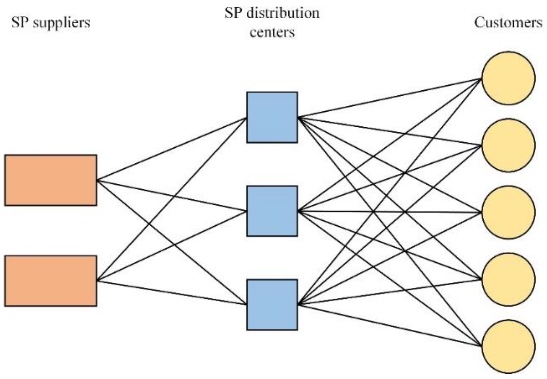
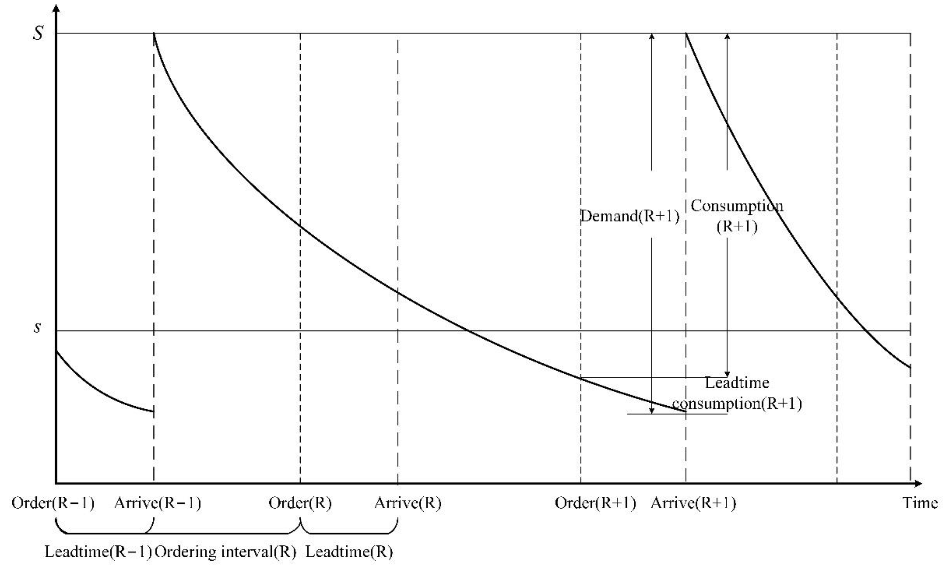
3.1. Problem Description

As is shown in Figure 1, the basic spare part supply chain network consists of spare part suppliers (SP suppliers), spare part distribution centers (SP distribution centers), and customers. The SP supplier provides spare parts for SP networks and satisfies spare part demand from the customer layer. The SP distribution center is responsible for spare part storage transported from the SP supplier and transshipment to the customer layer. The customer consumes spare parts and generates spare part demand. Each customer is made up of equipment inventory units and equipment maintenance units. In the equipment maintenance unit, spare part management is based on (T, s, S) inventory policy.
Figure 2 represents the (T, s, S) inventory control policy. The (T, s, S) inventory policy is an improvement based on the (s, S) inventory policy. Compared with the continuous review in (s, S) policy, this inventory policy adopts a period review. In the (T, s, S) inventory policy, the spare part stock level is checked at the end of an infinite review period. If the current stock level is less than or equal to the safety stock level s, a spare part order is generated. However, if the stock level is more than the safety stock level s, there are no spare part orders. The amount of ordered spare parts is aimed to satisfy the spare part consumption in this operating period and lead time. Therefore, the size of the spare part order should replenish the stock level in the arrival time to the maximum stock level S.
Based on the above description, the size of the spare part order depends on the consumption of the customer layer in terms of supply interval and lead time. The components of the equipment are usually subject to a fixed lifetime distribution. Accordingly, the number of damaged components in a fixed period of time can be calculated. With the component of equipment damaged, the equipment maintenance units adopt replacement, which removes damaged components and replaces them with corresponding new spare parts. It can be seen that the amount of spare part demand is equal to the damaged components.

3.2. Model Formulation

The probability calculation of spare part consumption s is as shown the following formula in a finite planning supply horizon h :
P s = F s h F s + 1 h
where F s h is the s -fold convolution of the cumulative failure distribution function F h . In order to reach the demand satisfaction level of customer k for spare parts, the amount of ordered spare parts can be calculated by the following formula:
P = s = 0 N P s = s = 0 N F s h F s + 1 h
where N is the spare part demand of the customer and also the spare part consumption in the finite horizon h .
The stock level change due to the spare part consumption of customer k is represented in Figure 2. The customers manage spare parts by the (T, s, S) inventory strategy. In Figure 2, the x-axis indicates the time process of the spare part supply, and the y-axis denotes the stock level change. The customer test stock level has an infinite period T. The τ th order period begins with the Order(R-1) moment and ends with Order(R). The spare part consumption in period τ consists of two components. One is the consumption in lead time, because there is a delay between placing spare part orders and the spare parts arriving, named delay consumption. The other is from spare parts arriving in the last supply period of spare part ordering, named general consumption.
The general spare part consumption in period τ can be calculated by Equation (3):
N k T k τ = n k inf N k T k τ P k s = 0 N k T k τ F s T L k τ 1 F s + 1 T L k τ 1
where N k T k τ represents the amount of general spare part consumption. L k τ 1 indicates the lead time of the τ 1 th ordering period.
The delay in the spare part consumption period τ can be obtained by Equation (4):
N k L k τ = n k inf N k L k τ P k s = 0 N k L k τ F s L k τ F s + 1 L k τ
where N k L k τ is the amount of delayed spare part consumption. L k τ shows the lead time of the τ th ordering period.
Based on Equations (3) and (4), the total spare part consumption can be calculated by the following equation:
N K τ = n k inf N K τ P k s = 0 N K τ F s T L k τ 1 + L k τ F s + 1 T L k τ 1 + L k τ

3.3. Mathematical Model

The spare part supply optimization model minimizes the total cost, which consists of the spare part transport cost, customer inventory cost, ordering cost from spare part suppliers, and downtime loss from the cost of the equipment. The objective function is calculated as follows:
min   Z τ = C t r a n s + C i n v e n t + C o r d e r + C d o w n
where
C τ t r a n s = i j sgn X i j τ C i j t r a n s + j k sgn X j k τ C j k t r a n s
C τ i n v e n t = k C k i n v e n t j X j k τ
C τ o r d e r = i C i o r d e r j X i j τ
C τ d o w n = k n k C k d o w n sgn - min S k N k τ , 0
Equation (6) represents the total cost of the spare part supply chain network in period τ . Formula (7) indicates the spare part transport cost in period τ , consisting of the transport process from SP suppliers to SP distribution centers and from SP distribution centers to customers. Equation (8) calculates the total spare part inventory cost for customers in period τ . The total spare part ordering cost from SP suppliers can be obtained by Equation (9).
Equation (10) formulates the downtime loss cost of the customers in a period τ . The following is the expression of the downtime loss. When spare part replacement caused by equipment failure and a spare part shortage happen at about the same time, customers will incur equipment downtime loss until the replenished spare parts arrive.
In Equation (10), sgn x is the step function, which is used to indicate a spare part shortage. When x is greater than zero, the function takes the value of one. When x is equal to zero, the value of the step function is equal to zero. When x is less than 0, the sign function takes the value of −1. It can be seen that if S k N k τ < 0 and min S k N k τ , 0 < 0 , then the current inventory level cannot satisfy the spare part consumption, which leads to a spare part shortage and equipment downtime loss. Therefore, sgn - min S k N k τ , 0 = 1 , which means customer k has spare part demands and the equipment downtown loss cost of customer k is n k C k d o w n . In other words, if S k N k τ 0 and min S k N k τ , 0 0 , then sgn - min S k N k τ , 0 = 0 , which indicates the current spare part stock is able to satisfy maintenance demand, and the customer will not incur a breakdown loss.
The corresponding constraints of the spare part supply optimization model are as follows:
y k τ = 1 I k τ s k 0 I k τ > s k
N K τ = n k inf N K τ P k s = 0 N K τ F s T L k τ 1 + L k τ F s + 1 T L k τ 1 + L k τ
d k τ = j X j k τ t r a n s = y k τ min N k τ , S k
i X i j τ k X j k τ
i X i j τ C a p j
L k τ = max T T i j t r a n s X i j τ + max T T j k t r a n s X j k τ
L k 0 = 0
sgn X i j τ = 1 X i j τ > 0 0 X i j τ = 0
sgn X j k τ = 1 X j k τ > 0 0 X j k τ = 0
X i j τ , X j k τ 0
Equation (11) is used to indicate whether spare part ordering happens at order point τ , while y k τ is an auxiliary binary variable. When the current spare part inventory level I k τ is less than or equal to the reorder point s k , y k τ = 1 , and the customer sends the spare part replenishment application. When I k τ is greater than s k , y k τ = 0 , and spare part orders will not happen in period τ . Equation (12) calculates the spare part consumption of customer k caused by equipment failure and replacement. Equation (13) is the demand constraint. On the one hand, the spare part inflow of customer k should be equal to the demand. On the other hand, spare part demand should be equal to the consumption in period τ .
The constraint in Equation (14) represents the flow balance constraint. The spare part inflow of SP distribution centers should be greater than or equal to the outflow. Equation (15) is the facility capacity constraint. The spare part inflow of SP distribution centers should not be more than the maximum capacity.
Equation (16) calculates the lead time in a period τ , which is equal to the sum of the transport time from an SP supplier to an SP distribution center and from an SP distribution center to a customer. Equation (17) indicates the lead time of the period 0, which is utilized to calculate the spare part consumption of the first period.
Equation (18) is utilized to indicate whether there is a spare part flow between the supplier i and the distribution center j . Equation (19) represents whether there is a spare part flow between the distribution j and customer k . Both of these equations are based on the sign function. If there is a spare part flow between two different echelons of facilities, then sgn X i j τ and sgn X j k τ take the value of one; otherwise, the value of sgn X i j τ and sgn X j k τ is equal to zero.
The constraint in Equation (20) indicates the variable characteristics.

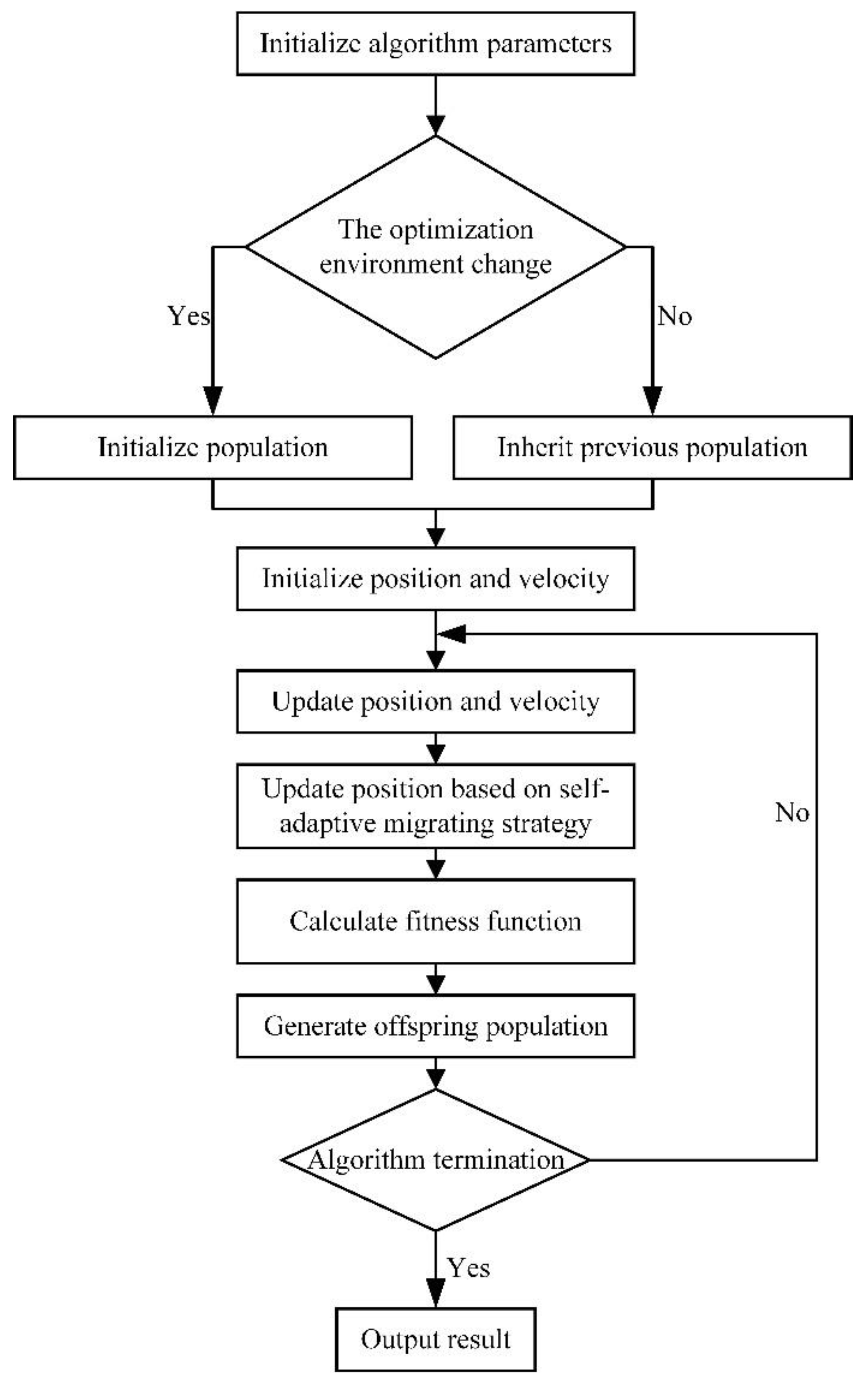
4. Self-Adaptive Dynamic Migrating Algorithm

The proposed mathematical model is a nonlinear integer programming problem. There are few appropriate and efficient exact algorithms for solving a complex nonlinear programming problem. However, meta-heuristic algorithms have been proven to efficiently solve nonlinear and complex optimization problems [11,28]. PSO, with its unique individual search mechanism and excellent population evolution method, is utilized to solve the proposed spare part supply optimization model.
The proposed multi-period spare part supply optimization model is a dynamic single-objective optimization problem. The spare part transportation lead time is different in each period, which leads to spare part demand changing with each period. Because the system parameters and corresponding constraints change in the multi-period dynamic optimization environment, the optimal population in the last period will be not suitable for the current optimization environment.
Compared to the dynamic optimization problem, the static optimization problem is solved in a fixed and static optimization environment. Therefore, the strategy for solving dynamic optimization problems is to divide them into several static optimization problems based on periodic steps. Then, the environment change detection mechanism and response mechanism are utilized to build a connection between several static optimization problems. The static optimization problem is solved by the proposed self-adaptive optimization algorithm. Therefore, the keys to solving dynamic optimization problems are an efficient environment change detection strategy and environment change response strategy.

4.1. Traditional Algorithm

The particle swarm algorithm, as a swarm intelligence optimization algorithm, simulates the bird swarm random search mechanism to solve a complex mathematical model. The random search is based on the global optimal position and personal optimal position. The position updating Equation (21) and velocity updating Equation (22) are as follows:
v i k + 1 = w v i k + c 1 r a n d 1 p b e s t k x i k + c 2 r a n d 2 g b e s t k x i k
x i k + 1 = x i k + v i k + 1
where v i k + 1 and v i k represent the search velocity of particle i in the k + 1 th and k th iterations, respectively, x i k + 1 and x i k indicate the current position of particle i in the k + 1 th and k th iteration, respectively, g b e s t k is the global optimal position of the whole particle population, p b e s t k is the personal optimal position of particle i , w is the inertia weight that controls the influence of the previous iteration of particles on the current particles, c 1 and c 2 are the cognitive learning coefficient and social learning coefficient, which measure the influence degree of the global best solution and personal best solution on the particles, respectively, and r a n d 1 and r a n d 2 are two different random numbers that are subject to uniform distribution. The flow chart of the traditional PSO algorithm is illustrated in Figure 3, and its special steps are illustrated as follows.
Step 1: Initialize the algorithm parameters: maximum iteration, population size, and individual dimension;
Step 2: Initialize the population;
Step 3: Initialize the position and velocity of the particle, the global best position, and the personal best position;
Step 4: Update the position and velocity of particles based on Equations (21) and (22);
Step 5: Calculate the fitness function value of each particle;
Step 6: Generate offspring populations by comparing fitness function superiority and inferiority relationships;
Step 7: Repeat steps 4–6 until the algorithm termination condition is met. Finally, output the optimal solution.
However, there are several disadvantages to the traditional PSO algorithm:
(1)
The values of some parameters should be set manually or obtained through extensive experiments. Therefore, in the case of several parameters involved, the optimal combination is difficult to determine, especially when solving multi-period dynamic optimization problems. For dealing with the above problems, most of the research proposed some methods, such as a self-adaptive strategy [40,41,42].
(2)
When solving complex and nonlinear programming models, the PSO algorithm may fall into local convergence. It is expected that the PSO algorithm has excellent population diversity by global searching in the initial iteration and an excellent local search ability for better convergence in later iterations. There are also many strategies such as the levy fly strategy based on the self-adaptive fly probability [11].

4.2. Environment Change Detection and Response Mechanism

The optimization environment will change with the system parameters changing in multi-period dynamic optimization problems. The environment change detection mechanism and response mechanism are the most important parts of the dynamic optimization algorithm. Most of the detection mechanisms are utilized to detect the environmental change; that is to say, compared with the previous period, they detect whether the optimization environment and function mapping relation change at the current moment.
There are two kinds of common detection mechanisms: reevaluating partial particles and estimating the fitness function distribution of the population. Both detection mechanisms need to reevaluate and verify the fitness function values of the population so as to result in the high computational complexity of the dynamic PSO algorithm. Therefore, a system parameter-based environment change detection factor is proposed. This detection factor directly detects the possible change in system parameters instead of partial particles or the particle population:
D e t e c t o r t = m = 1 M 1 sgn C m t C m t 1
Suppose that there are M system parameters in the proposed spare part supply optimization model. C m τ represents the system parameter of the t th iteration, while C m τ 1 indicates the parameters of the t 1 th iteration. The sign function is utilized to measure whether the system parameter of the current iteration is compared with the previous iteration. For a single system parameter, when the m th system parameter changes, the sign function is equal to one, and when this parameter does not change, the sign function takes the value of zero. For all system parameters, if any of the system parameters change, the D e t e c t o r t takes the value zero. Only when there are no system parameters that change is the value of D e t e c t o r t one.
Furthermore, the environment change response mechanism is the key to designing the dynamic PSO algorithm. When the optimization environment changes, the optimal particle population in the previous optimization environment does not apply to the new optimization environment. The response strategy is utilized to update the population so as to make the new population rapidly converge to the optimal solution. The most common response strategies are randomly initializing the population and inheriting the optimal population.
The environmental change in the spare part supply system follows a periodic pattern such that the optimal population in the previous environment has an influence on the new environment and provides some information corresponding to population evolution. However, in the proposed supply chain network optimization model, the lead time, as a critical parameter, guides the evolution of the particles and is utilized to calculate other important parameters, such as consumption and demand. Therefore, in this paper, for improving the population diversity, a randomly initialized particle population is considered for the environment change response strategy.

4.3. Self-Adaptive Nonlinear Decreasing Inertia Weight

The inertia weight w controls the influence of previous particles on the current particles. In the process of PSO optimization, an inappropriate inertia weight will decrease the convergence rate and have a negative influence on the algorithm’s performance. Therefore, a self-adaptive nonlinear decreasing strategy for determining the inertia weight is proposed in this research. This self-adaptive nonlinear decreasing strategy determines the value of the inertia weight w based on the current algorithm iteration. Equation (24) calculates the self-adaptive inertia weight:
w = w max + w min w max cos π 2 i t e r M a x i t e r
where w min is the minimum inertia weight and w max is the maximum inertia weight. With the variable ranging from 0 to π / 2 , the value of the cosine function is small and decreases rapidly in the early iteration, while it is large and decreases slowly in the later iteration.

4.4. Self-Adaptive Nonlinear Migrating Strategy

For dealing with the local convergence and avoiding premature phenomena, a self-adaptive nonlinear migrating strategy based on biological migration behavior was adopted to improve PSO performance. The migrating strategy is widely utilized to improve the global search ability of swarm intelligence algorithms. For example, the seagull optimization algorithm and sooty tern optimization algorithm introduce bird migration behavior to simulate global searching [43,44].
The process of particle migration happens after the position and velocity of the particle are updated based on Equations (21) and (22) in each iteration. The migrating behavior consists of three stages: collision avoidance, the movement toward the direction of the best particle, and updating close to the best particle.
Step 1: Collision avoidance
For avoiding a collision with the neighbor (other particles), an additional variable A is adopted to calculate the new particle position:
C i i t e r = A P i i t e r
where C i i t e r represents the particle position that does not collide with other particles, P i i t e r denotes the current position of the particle, i t e r indicates the current number of iterations, and A represents the particle movement in an infinite search space:
A = f c f c i t e r / M a x i t e r
In Equation (26), f c is a control variable to adjust the frequency of employing particle movement A , which decreases linearly from f c to 0 in the traditional migration strategy. The above process is presented in Figure 4.
Step 2: The wolves moving toward the direction of the best particle
In the case of avoiding a collision in the particle swarm, the particle population converges toward the direction of the best particle position:
M i = B P b e s t i t e r P i i t e r
Equation (27) indicates the position movement of particle P i toward the position of the best particle P b e s t . B is responsible for seeking a trade-off between the exploration ability and exploitation ability:
B = 2 A r a n d
where r a n d is a random number that is subjected to the uniform distribution.
The above process is presented in Figure 5.
Step 3: Update close to the best particle
Finally, particle i is guided by the best particle position, and its position is updated:
D i i t e r = C i i t e r + M i i t e r
where D i i t e r is the updated position of the particle. Based on Equations (25) and (27), Equation (28) can be transferred to the following form:
D i i t e r = A P i i t e r + 2 A r a n d P b e s t i t e r P i i t e r
The above process is presented in Figure 6.
Step 4: The self-adaptive nonlinear weight coefficient
However, compared with the linear decreasing of the weight coefficient, the nonlinear decreasing method can efficiently improve the global search ability [45]. A nonlinear decreasing strategy based on the cosine function is improved in this research:
A = f c f c cos π 2 i t e r M a x i t e r
Through the cosine function, in the early iteration, the influence of the best particle position on the current position is weakened so as to improve the early global search performance. With the PSO algorithm iteration process going on, the influence of the best particle is strengthened, which leads to other particles moving toward the direction of the best particle.

4.5. Pseudocode Implement

The flow chart of the proposed improved self-adaptive dynamic migrating PSO algorithm is shown in Figure 7, and its specific steps are as follows:
Step 1: Initialize the algorithm parameters: maximum iteration, population size, and individual dimension.
Step 2: Detect whether the optimization environment changes based on the proposed environment change detection mechanism. If the environment changes, then initialize the population; otherwise, inherit the previous population.
Step 3: Initialize the position and velocity of the particle, the global best position, and the personal best position.
Step 4: Update the position and velocity of the particles based on Equations (21) and (22).
Step 5: Update the positions of the particles according to the self-adaptive migrating strategy.
Step 6: Calculate the fitness function value of each particle.
Step 7: Generate offspring populations by comparing fitness function superiority and inferiority relationships.
Step 8: Repeat steps 4–7 until the algorithm termination condition is met. Finally, output the optimal solution.

4.6. Fitness Function Calculation

The proposed nonlinear optimization model is a single-objective optimization model with equality constraints and inequality constraints. Hence, the fitness function is calculated as the sum of the objective function and total constraint violations:
f x = O x + M V x
where O x represents the objective function, V x indicates the total constraint violations, and M is the constraint penalty coefficient, which is utilized to measure the degree to which the individual conforms to the constraints.
On the basis of the constraints set in the proposed model, the constraint violation function V x is defined in the following form:
V x = l = 1 L C l x
where L is the number of constraints. Suppose that g l x is the equality constraints and h x is the inequality constraints. C l x is calculated by Equation (33):
C l x = max g l x , 0 g l x 0 max h l 2 x , 0 h l x = 0

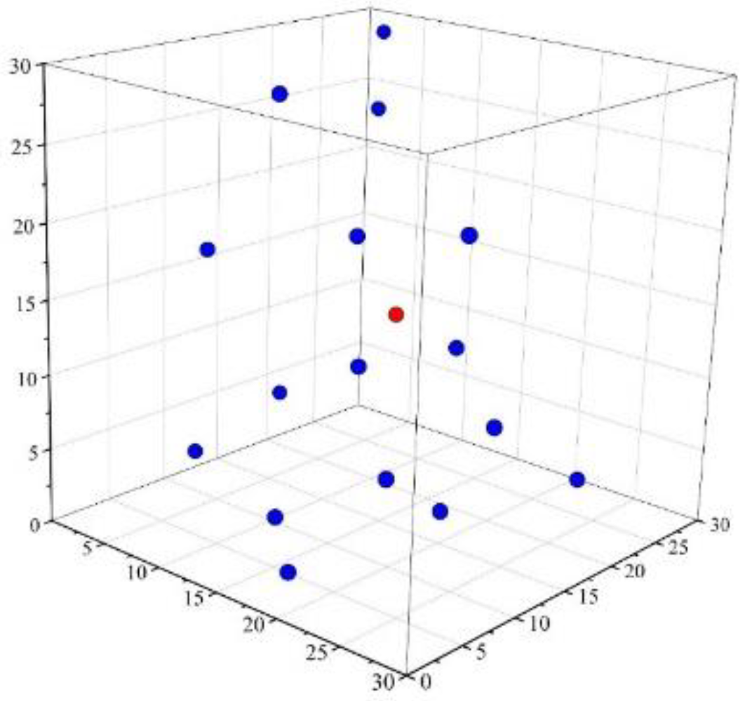
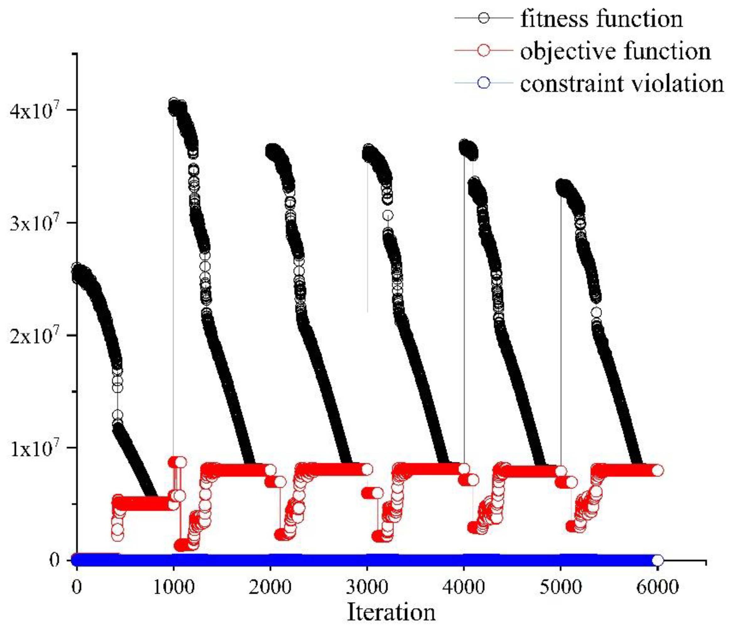
5. Numerical Experiment

5.1. Case Description

This section represents a set of numerical instances for validating the proposed spare part supply chain network optimization model and improved SDMPSO. In our numerical case, one SP supplier, three SP distribution centers, and six customers were predetermined to make up the three-echelon spare part supply chain network. When equipment fell into failure and needed components replaced, replacement repair was adopted. The lifetime distributions of the corresponding components and spare parts were known and are represented in Table A1 of the Appendix A.
Table A2, Table A3 and Table A4 in the Appendix A represent some parameters involving the three-echelon spare part supply chain network under the (T, s, S) inventory control policy. Table A2 consists of the amount of equipment n k for the customers, the reorder stock level s k , the maximum stock level S k , the values of the standard normal distribution μ k , and the demand fill rate P k . The various costs related to supply and inventory are shown in Table A2, Table A3 and Table A4. The inventory cost and downtime loss for customers are represented in Table A2. The transportation costs between two different echelons of facilities are shown in Table A3. Table A4 indicates the transportation times from the suppliers to the distribution centers and from the distribution centers to customers. It should be mentioned that because of random disruptions in the transportation system, the value of the transportation time is supposed to be subject to uniform distribution. Therefore, the spare part ordering cost C i o r d e r in the supplier took on a value of 1000.
The whole spare part supply planning horizon was divided into six periods, and each period was set to 5000 h. The proposed optimization model was solved on a laptop computer with an Intel(R) Core(TM) i7-6700HQ CPU @ 2.60GHz and 16.00 GB RAM environment.
The algorithm parameters of the proposed SDMPSO are as follows: maximum iteration number = 1000, maximum inertia weight = 0.9, minimum inertia weight = 0.4, population size = 150, individual dimension = 21, cognitive learning coefficient = 1.4962, social learning coefficient = 1.4962, and fixed inertia weight = 0.7298.

5.2. Results Analyses

The multi-period spare part supply chain network optimization model was solved by the proposed SDMPSO. The experiment was carried out five times. In Figure 8, the black part represents the convergence curves of the algorithm fitness function, the red part indicates the objective function, and the blue part is the total constraint violation. The x-axis indicates the current number of algorithm iterations, and the y-axis represents the corresponding value of the corresponding function. Because the optimization environment changed every 1000 iterations, the coordinate scales of the x-axis were spaced 1000 places apart.
As is shown in Figure 8, in each supply period, all of the fitness functions could be converged at the end of the period. Meanwhile, the global optimal solution could be obtained. Moreover, it can be seen in Figure 8 that the values of the fitness function were equal to the values of the objective function when the iteration of each period was completed, and the total constraint violation is equal to 0 in Figure 8. Both of the aforementioned phenomena show that the obtained optimal solution is feasible at the beginning of each period.
The results of the obtained optimal solution are shown in Table 2 which consists of the cost of each period, the total cost of the entire horizon, the spare part consumption of each period, the lead times of each period, and the breakdown loss of each period. As can be seen in Table 2, there was spare part replenishment ordering in each period, which shows that the predetermined reorder stock level was reasonable. The consumption of each period was equal to or more than the difference between the reorder stock level s k and the maximum stock level S k . It can be seen that the down losses were equal to zero, which shows that there were no spare part shortages in each period. Therefore, compared with other periods, the first period had more spare part consumption. The reason for the aforementioned phenomenon is that the length of the first period was 5000 h.

5.3. Sensitivity Analyses

This section is dedicated to performing sensitivity analyses on critical model parameters and improved algorithm strategies, which are illustrated in Table 3.

5.3.1. Two Kinds of Inventory Policy

In this section, two different inventory control policies are utilized to perform sensitivity analysis. Model 1 represents the proposed model in Section 3. The spare part consumption during the lead time was not taken into consideration in model 2, which is shown in the following equation:
N K τ = n k inf N K τ P k s = 0 N K τ F s T F s + 1 T
As is shown in Table 4, there was a large number of equipment breakdowns in each period on the basis of model 2. Moreover, compared with the traditional (T, s, S) inventory control policy, the improved (T, s, S) policy could save more in terms of spare part supply costs and breakdown losses.

5.3.2. Sensitivity Analyses of the Failure Rate

In this section, for analyzing the impact of the equipment failure rate λ on the spare part supply process, the model is solved with different values for the failure rate, and the obtained results are shown in Table A5 of the Appendix A. The failure rates took on the values of 1 × 10⁻⁴, 1.25 × 10⁻⁴, 1.5 × 10⁻⁴, 2 × 10⁻⁴, 4 × 10⁻⁴, and 6 × 10⁻⁴. It can be seen in Table A5 that with the increase in the equipment failure rate, spare part consumption increased. This is because the greater failure rate resulted in more equipment falling into failure and more repair demands. Secondly, when the failure rate reached 2 × 10⁻⁴, there were breakdown losses. In this case, an excessive failure rate led to too much equipment falling into failure. Therefore, too many repair demands led to the spare part inventory for customers running out, causing the breakdown of the equipment and resulting in breakdown losses. Thirdly, the total cost of the excessive failure rates was greater than the cost without equipment breakdowns happening.
As is illustrated in the expected cost of Table A1, the total cost in the entire planning horizon increased with the equipment failure rate increasing. Therefore, in real-world spare part inventory control and supply, equipment breakdowns should be eliminated as much as possible, or the breakdown time should be decreased by timely replenishment and safe stock levels. On the other hand, the equipment failure rate should be decreased by some efficient methods, such as preventive maintenance.

5.3.3. Sensitivity Analyses of the Reorder Stock Level

This section is dedicated to analyzing the impact of the reorder stock level on spare part inventory control and supply. For this purpose, the model was solved according to five scenarios based on different reorder stock levels (−3, −6, based case, +3, and +6), and the results are shown in Table A6 of Appendix A. The reorder stock level is utilized to determine whether a spare part replenishment order is placed. As is depicted in Table A6, there was an equipment breakdown in the first period of scenario 1. This is because too low a reorder stock point will determine that spare part replenishment is not needed. However, the surplus inventory in the previous period cannot satisfy the spare parts consumption in the current period.
The expected cost of Table A6 shows the change in the expected total cost in the entire planning horizon with the reorder stock level increasing. In scenarios 1–3, increasing the reorder stock level led to an increase in the total cost. A lower reorder stock level would induce fewer spare part replenishment times so as to lessen the cost. However, the probability of equipment breaking down would increase. On the other hand, increasing the reorder stock level resulted in a decrease in the total cost from scenario 3 to scenario 5. An excessive reorder stock level leads to more ordering times but decreases the order quantity in spare part replenishment. Hence, setting up a reasonable reorder stock level can improve the economic performance of the spare part supply network.

5.3.4. Maximum Stock Level

This section is dedicated to performing sensitivity analyses on the maximum stock level in five scenarios over the planning horizon (−5, −10, base case, +5, and +10). The obtained results are represented in Table A7 of Appendix A.
Table A7 shows that there were equipment breakdowns in scenario 1 and scenario 2. The above phenomenon is because, in the case of the same spare part consumption, the scenarios with lower maximum inventory stock levels could not afford the repair demands. As is illustrated by the expected cost in Table A7, the increase from scenario 1 to scenario 3 led to a small increase in the total cost. This is because the lower maximum stock level resulted in more replenishment order times with small order quantities. On the contrary, the increase from scenario 3 to scenario 5 led to a decrease in the total cost over the planning horizon. Based on the analyses of the aforementioned results, the impact of the maximum stock level on the total cost is nonlinear and monotone, so the maximum stock level should be reasonable.

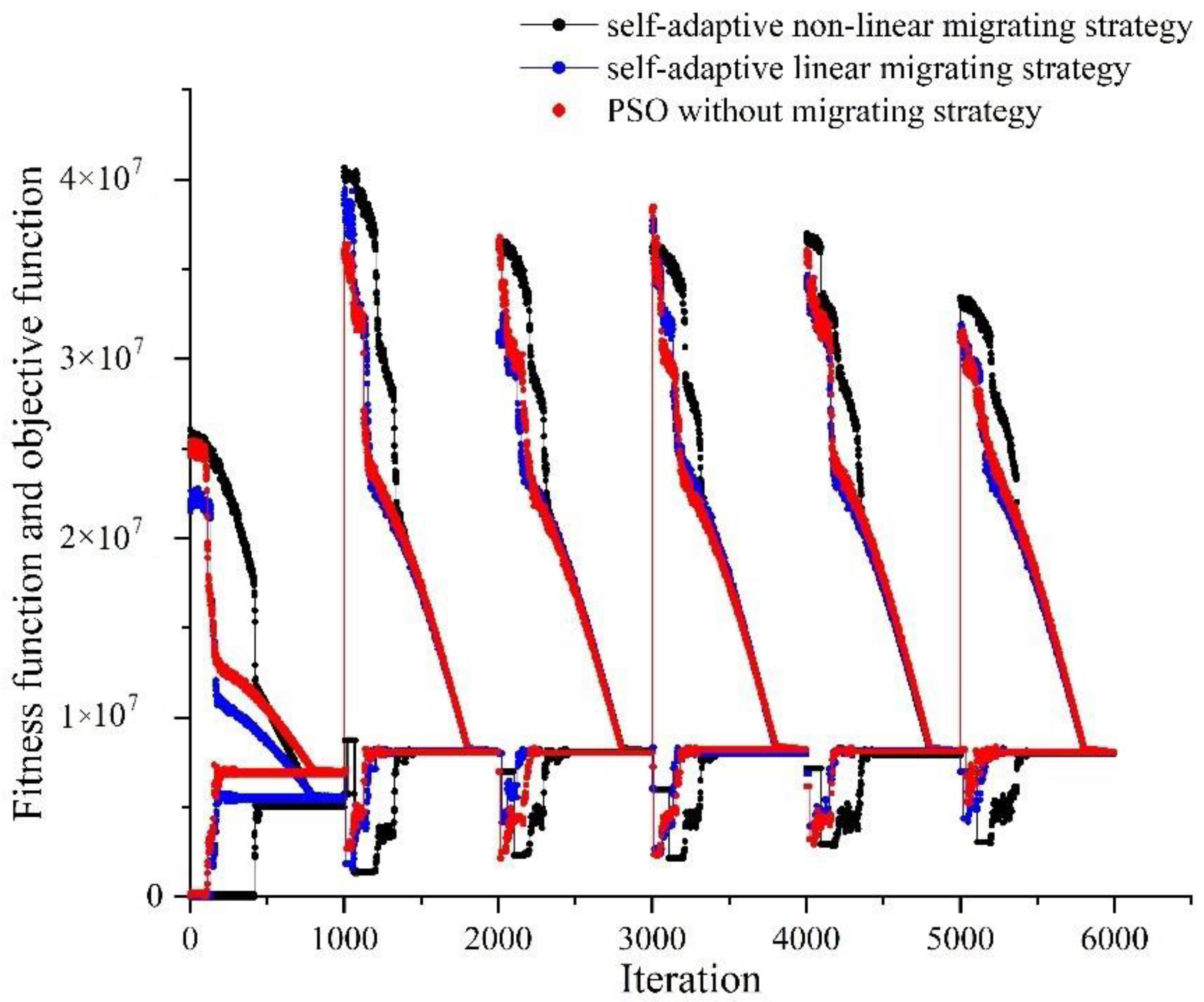
5.4. Algorithm Efficiency Analyses

This section is dedicated to performing sensitivity analyses for investigating algorithm performance under different strategies. The proposed SDMPSO adopts the self-adaptive nonlinear decreasing inertia weight and self-adaptive nonlinear migrating strategy. The following results from the analyses were determined to evaluate algorithm efficiency based on different inertia weight strategies and different migrating strategies.

5.4.1. Migrating Strategy

In the first section, on the basis of adopting the same self-adaptive nonlinear decreasing inertia weight strategy, three different migrating strategies were utilized to investigate the performance of SDMPSO. For this purpose, the self-adaptive nonlinear migrating strategy, self-adaptive linear migrating strategy, and the improved PSO without migrating strategy were investigated.
It can be seen from Figure 9 that the algorithms with the three migrating strategies could be converted to the optimal solutions. Moreover, from Figure 9, the fitness value of the nonlinear migrating strategy was greater than PSO with and without the linear migrating strategy.
It can be seen in Table 5 that the CPU time of the algorithm with the migrating strategy was greater than that without the migrating strategy, which shows that PSO with the migrating strategy had a more excellent calculation efficiency and convergence rate. Moreover, PSO with an improved nonlinear migrating strategy had less CPU time than that with a traditional linear migrating strategy, which proves the effectiveness of improved SDMPSO. The results show that the improved algorithm improved the computation time by 8 percent compared with the traditional algorithm.

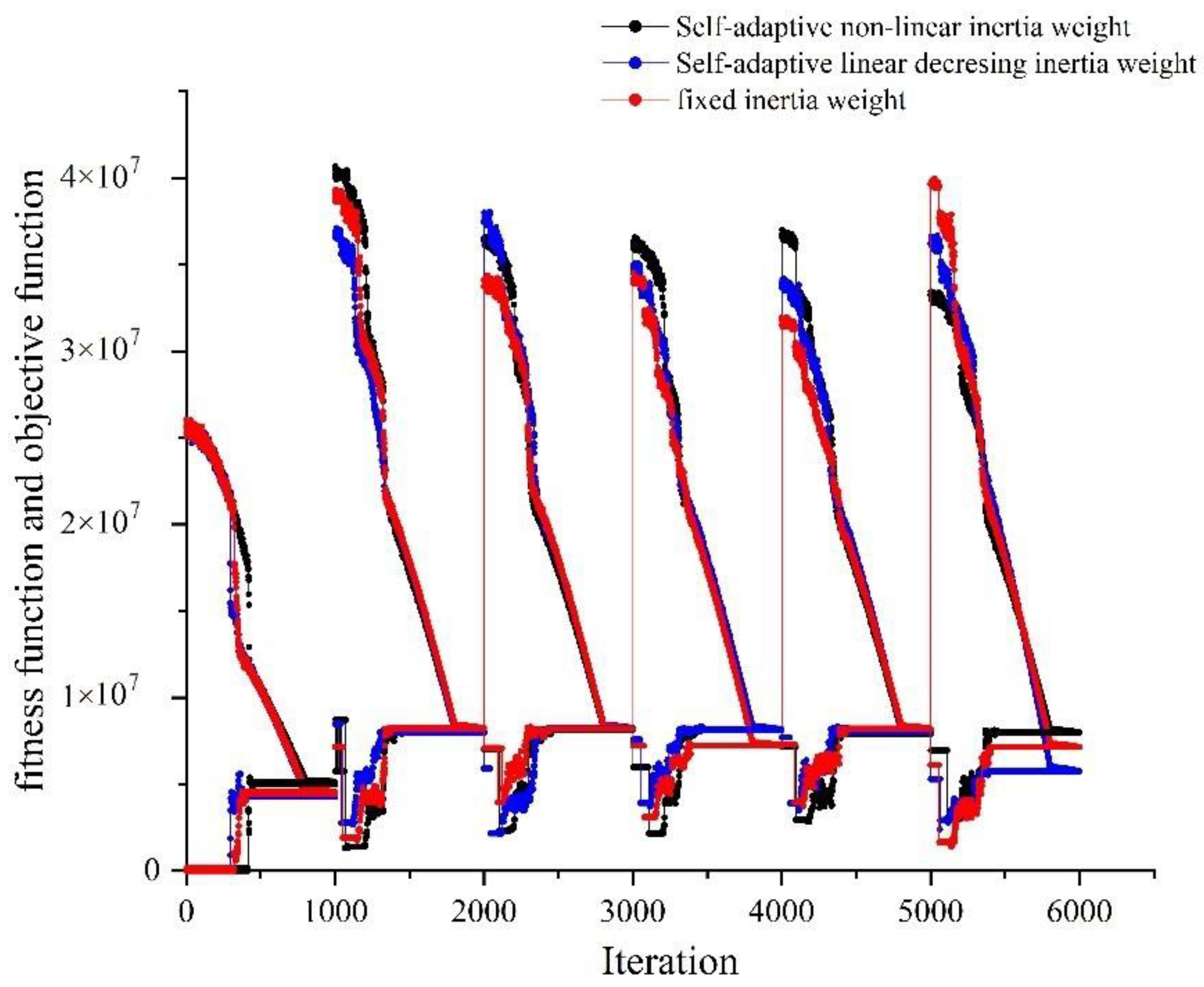
5.4.2. Inertia Weight

In this section, the obtained results and CPU times of three different inertia weight strategies are compared in the case of adopting the same self-adaptive nonlinear migrating strategy. The three inertia weight strategies were the proposed nonlinear decreasing inertia weight, linear decreasing inertia weight, and fixed inertia weight. As is shown in Table 6, the CPU time of SDMPSO was greater than that of PSO with the linear decreasing strategy or fixed inertia weight, which was due to the characteristic of the cosine function shown in Section 4.5.
Figure 10 shows the convergence curve of the objective function and fitness function with three different inertia weight strategies. The x-axis denotes the number of iterations. The y-axis indicates the value of the objective function and fitness function. In Figure 10, the three inertia weight strategies have similar convergence curves. Therefore, in the case of the three strategies, the obtained optimal solutions were feasible. The different inertia weight strategy had a more positive influence on the convergence velocity but less impact on the population diversity.

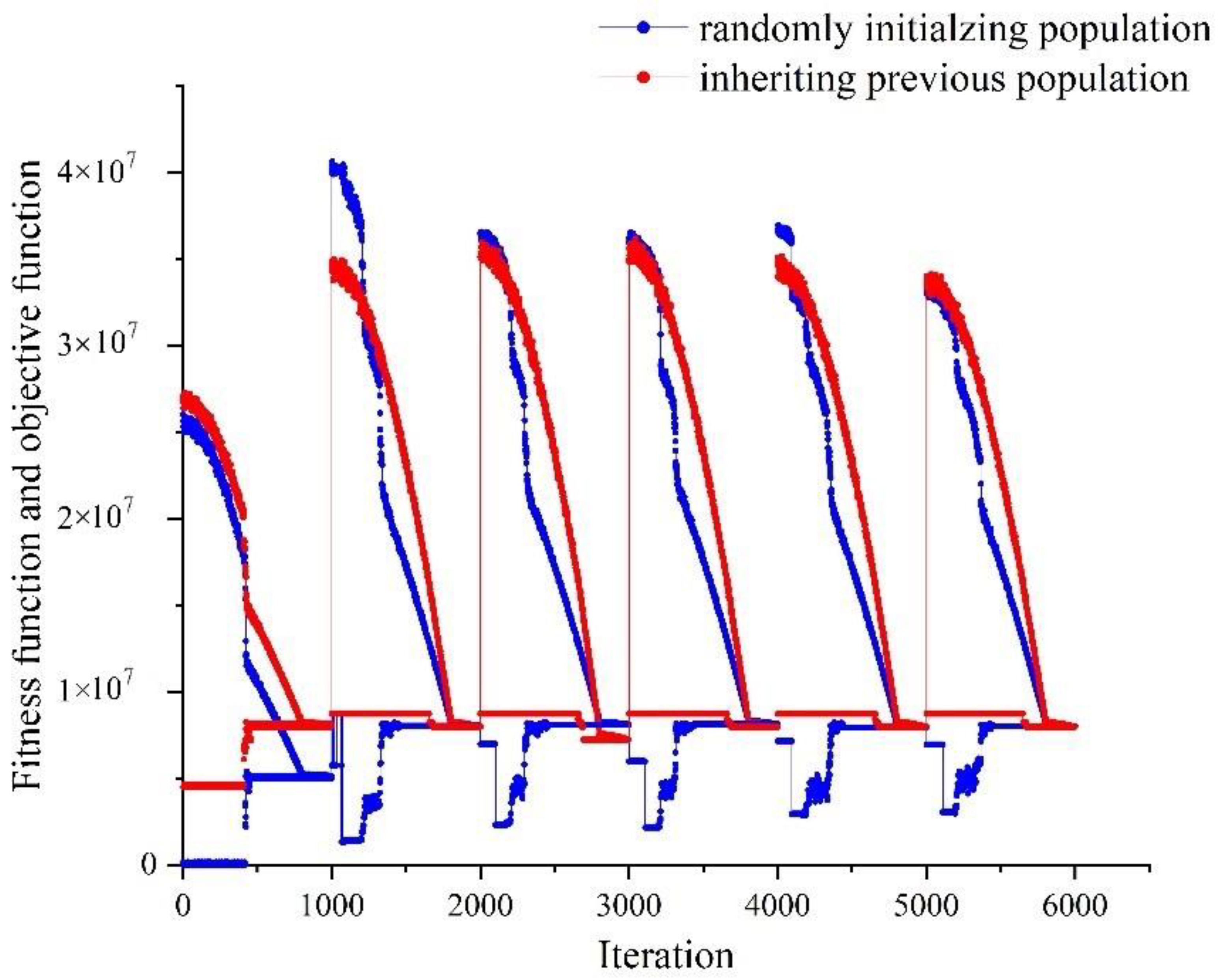
5.4.3. Response Strategy

This section is dedicated to performing algorithm efficiency analyses for comparing two different response strategies. The environment response strategy was determined by the characteristics of dynamic optimization problems. Hence, randomly initializing the population strategy (strategy 1) and the inheriting of a previous population strategy (strategy 2) were utilized to investigate the validity and suitability of different response strategies. For avoiding early local convergence, a self-adaptive nonlinear migrating strategy was utilized to improve the population diversity after detecting the environmental change. The obtained results are shown in Figure 11. Figure 11 depicts that the algorithm with two response strategies could be converged to the global optimal solutions. However, in the case of inheriting the previous population, after progressing to the next period, the algorithm could rapidly search for the optimal solution.

6. Conclusions

This research addresses a multi-period multi-echelon spare part supply chain network optimization problem under the (T, s, S) inventory control policy. A period review with a variable order quantity strategy was utilized to determine the supply time, amount of spare part demand, and lead time. Based on the (T, s, S) inventory control policy and three-echelon spare part supply chain network, a joint optimization model of inventory and supply was proposed. However, the model is a nonlinear, non-convex, and multi-period dynamic problem, so it is difficult to seek a traditional method to solve it. An improved PSO named SDMPSO with a novel environment change detection strategy was proposed. For improving the convergence velocity, a self-adaptive nonlinear decreasing inertia weight strategy was adopted into an improved PSO algorithm. For balancing the population diversity and convergence efficiency, a self-adaptive nonlinear migrating strategy was adopted. The proposed model and improved algorithm were validated by a numerical case study. The parameter sensitivity analyses can provide a reference for real-world spare part management, such as reasonable maximum stock levels and reorder stock points. The algorithm efficiency analyses proved the improved SDMPSO’s superiority and correctness.
In this paper, the equipment was considered to be subject to exponential distribution. Future research can focus on different lifetime distributions, such as the Weibull distribution. Furthermore, some spare part demand may be emergent, so emergency distribution from suppliers to customers and the lateral transition between customers can be taken into consideration in designing a spare part supply chain network.

Author Contributions

Conceptualization, Y.G. and Q.S.; methodology, Y.G.; software, Y.G.; validation, Q.S.; formal analysis, Y.G.; investigation, Y.G.; resources, C.G.; data curation, C.G.; writing—original draft preparation, Y.G.; writing—review and editing, C.G.; visualization, Y.G.; supervision, Q.S.; project administration, Q.S.; funding acquisition, C.G. All authors have read and agreed to the published version of the manuscript.

Funding

This research was funded by The National Natural Science Foundation of China, grant number 71871220.

Data Availability Statement

The data presented in this study are available on request from the corresponding author.

Acknowledgments

Our deepest gratitude goes to the anonymous referees for detailed reviews and insightful comments that have helped improve this research substantially. This study was supported by The National Natural Science Foundation of China under grant number 71871220. This support is gratefully appreciated.

Conflicts of Interest

The authors declare no conflict of interest.

Abbreviations

i Index of SP supplier, where i = 1 , 2 , , I
j Index of SP distribution centers, where j = 1 , 2 , , J
k Index of customers, where k = 1 , 2 , , K
T The SP ordering interval
τ The SP supply period
H The entire SP supply planning horizon
s k The reorder stock level of a customer k
S k The maximum stock level of a customer k
n k Amount of equipment with a customer k
F h The cumulative failure distribution function of a spare part
f h The probability density function of spare part failure
C i j t r a n s Transport cost of a unit in kg of spare parts from SP supplier i to SP distribution center j
C j k t r a n s Transport cost of a unit in kg of spare parts from SP distribution center j to customer k
C k i n v e n t Inventory cost of a unit of spare parts for customer k
C i o r d e r Ordering cost of a unit of spare parts for SP supplier i
C k d o w n Downtime loss cost of a unit of equipment for customer k
C a p j Maximum capacity of SP distribution center j
I k τ Spare part inventory level of a customer k at τ moment
T T i j t r a n s Transport time of a unit of spare parts from SP supplier i to SP distribution center j
T T j k t r a n s Transport time of a unit of spare parts from SP distribution center j to customer k
L k 0 Leadtime of period zero
d k τ Spare part demand of customer k in period τ
i X i j τ Number of spare parts transported from SP supplier i to SP distribution center j in period τ
k X j k τ Number of spare parts transported from SP distribution center j to customer k in period τ

Appendix A

Table A1. Parameters of spare part lifetime distribution.
Failure   Rate   ( λ ) 2 × 1 0 - 4
Cumulative distribution function F t = 1 e λ t
N convolution of cumulative distribution function F s t = n s 1 1 n ! λ t n e λ t
Table A2. Parameters of spare part supply network and inventory control policy.
n k s k S k P k μ k C k i n v e n t C k d o w n
Customer 111308599.60%2.6520017,500
Customer 210308899.95%3.2822018,000
Customer 35358599.83%2.9320020,000
Customer 48359099.77%2.8421012,000
Customer 512349698.87%2.2825010,000
Customer 610288099.96%3.3322515,000
Table A3. Transportation cost of unit spare parts.
SupplierCustomer 1Customer 2Customer 3Customer 4Customer 5Customer 6
Distribution center 18008555951008580
Distribution center 210008075857585105
Distribution center 39501008090808095
Table A4. Transportation time between two echelons of facilities.
SupplierCustomer 1Customer 2Customer 3Customer 4Customer 5Customer 6
Distribution center 1U(1450,1500)U(45,50)U(15,20)U(25,30)U(35,40)U(45,50)U(25,30)
Distribution center 2U(1550,1600)355025202540
Distribution center 3U(1650,1700)154040304045
U indicates that this parameter is subject to the uniform distribution.
Table A5. Results for different equipment failure rates.
λ Total CostExpected CostConsumptionLead TimeDown Loss
12,703,64923,796,103 [54, 50, 25, 40, 60, 50] [1705, 1705, 1694, 1694, 1705, 1704] [0, 0, 0, 0, 0, 0]
3,738,404 [45, 51, 25, 30, 49, 50] [1713, 1712, 1702, 1701, 1711, 1713] [0, 0, 0, 0, 0, 0]
4,965,303 [44, 50, 25, 31, 49, 48] [1722, 1718, 1709, 1711, 1720, 1718] [0, 0, 0, 0, 0, 0]
3,384,491 [43, 49, 25, 31, 47, 50] [1719, 1715, 1708, 1708, 1715, 1715] [0, 0, 0, 0, 0, 0]
3,924,143 [43, 50, 25, 33, 48, 51] [1699, 1696, 1688, 1687, 1696, 1696] [0, 0, 0, 0, 0, 0]
5,080,113 [44, 51, 25, 32, 47, 50] [1713, 1715, 1704, 1701, 1713, 1716] [0, 0, 0, 0, 0, 0]
1.255,721,33331,687,145 [56, 61, 25, 40, 61, 61] [1701, 1702, 1691, 1690, 1704, 1701] [0, 0, 0, 0, 0, 0]
5,230,245 [55, 51, 25, 39, 49, 50] [1720, 1719, 1713, 1709, 1720, 1722] [0, 0, 0, 0, 0, 0]
6,277,729 [56, 49, 25, 40, 48, 50] [1742, 1743, 1731, 1730, 1741, 1744] [0, 0, 0, 0, 0, 0]
4,646,364 [57, 49, 25, 40, 50, 51] [1734, 1732, 1723, 1724, 1734, 1732] [0, 0, 0, 0, 0, 0]
6,059,167 [56, 51, 25, 40, 48, 51] [1742, 1747, 1733, 1736, 1747, 1747] [0, 0, 0, 0, 0, 0]
3,752,307 [54, 50, 25, 40, 46, 49] [1699, 1699, 1689, 1687, 1700, 1696] [0, 0, 0, 0, 0, 0]
1.51,319,57222,641,861 [66, 59, 30, 48, 61, 60] [1721, 1721, 1708, 1707, 1718, 1721] [0, 0, 0, 0, 0, 0]
1,977,966 [55, 50, 25, 41, 61, 51] [1732, 1736, 1723, 1727, 1736, 1735] [0, 0, 0, 0, 0, 0]
4,454,049 [55, 48, 25, 39, 61, 51] [1737, 1737, 1732, 1728, 1740, 1741] [0, 0, 0, 0, 0, 0]
5,993,321 [57, 49, 25, 40, 60, 50] [1735, 1735, 1729, 1726, 1738, 1736] [0, 0, 0, 0, 0, 0]
5,668,622 [57, 51, 25, 41, 59, 49] [1699, 1704, 1692, 1694, 1700, 1700] [0, 0, 0, 0, 0, 0]
3,228,331 [54, 51, 25, 40, 61, 50] [1739, 1736, 1729, 1728, 1739, 1737] [0, 0, 0, 0, 0, 0]
24,993,06445,154,757 [66, 80, 35, 55, 73, 79] [1721, 1720, 1707, 1711, 1719, 1718] [0, 0, 0, 0, 0, 0]
8,023,943 [55, 71, 35, 41, 59, 68] [1718, 1717, 1705, 1705, 1717, 1716] [0, 0, 0, 0, 0, 0]
8,102,537 [53, 68, 35, 48, 60, 69] [1743, 1744, 1736, 1735, 1747, 1744] [0, 0, 0, 0, 0, 0]
8,135,761 [56, 71, 35, 49, 59, 71] [1734, 1734, 1722, 1725, 1731, 1730] [0, 0, 0, 0, 0, 0]
7,907,696 [55, 71, 34, 39, 60, 70] [1712, 1711, 1699, 1701, 1713, 1709] [0, 0, 0, 0, 0, 0]
7,991,756 [57, 70, 34, 39, 60, 70] [1722, 1720, 1713, 1713, 1721, 1720] [0, 0, 0, 0, 0, 0]
48,574,06350,582,426 [98, 109, 54, 89, 109, 108] [1732, 1732, 1721, 1721, 1731, 1730] [192,500, 180,000, 0, 0, 120,000, 150,000]
5,468,600 [89, 97, 45, 71, 85, 100] [1712, 1714, 1706, 1705, 1713, 1716] [192,500, 180,000, 0, 0, 0, 150,000]
9,179,877 [90, 99, 46, 72, 84, 102] [1733, 1730, 1723, 1723, 1733, 1733] [192,500, 180,000, 0, 0, 0, 150,000]
9,192,362 [88, 98, 45, 72, 86, 100] [1702, 1700, 1692, 1690, 1699, 1703] [192,500, 180,000, 0, 0, 0, 150,000]
9,084,593 [88, 98, 45, 72, 86, 100] [1709, 1712, 1701, 1702, 1712, 1710] [192,500, 180,000, 0, 0, 0, 150,000]
9,082,931 [86, 101, 46, 71, 84, 102] [1733, 1729, 1719, 1720, 1732, 1732] [192,500, 180,000, 0, 0, 0, 150,000]
68,648,92548,814,486 [131, 141, 66, 97, 131, 141] [1721, 1722, 1710, 1710, 1722, 1717] [192,500, 180,000, 0, 96,000, 120,000, 150,000]
8,447,030 [107, 122, 55, 82, 120, 123] [1708, 1711, 1701, 1699, 1708, 1708] [192,500, 180,000, 0, 0, 120,000, 150,000]
8,513,053 [112, 117, 58, 81, 123, 123] [1744, 1746, 1737, 1733, 1743, 1745] [192,500, 180,000, 0, 0, 120,000, 150,000]
6,172,042 [113, 122, 55, 79, 122, 119] [1698, 1701, 1688, 1691, 1698, 1698] [192,500, 180,000, 0, 0, 120,000, 150,000]
8,524,459 [111, 119, 61, 80, 123, 118] [1736, 1738, 1727, 1727, 1735, 1736] [192,500, 180,000, 0, 0, 120,000, 150,000]
8,508,977 [112, 119, 59, 79, 121, 121] [1742, 1740, 1734, 1731, 1745, 1744] [192,500, 180,000, 0, 0, 120,000, 150,000]
Table A6. Results for different reorder stock levels.
ScenariosTotal CostExpected CostConsumptionLead TimeDown Loss
1241,379,85440,677,712 [67, 81, 35, 56, 73, 80] [1732, 1729, 1721, 1722, 1729, 1732] [0, 0, 0, 0, 0, 0]
247,540,815 [55, 70, 35, 46, 59, 72] [1716, 1718, 1707, 1707, 1714, 1715] [0, 0, 0, 0, 0, 0]
297,937,264 [54, 69, 35, 47, 59, 70] [1743, 1741, 1729, 1733, 1739, 1742] [0, 0, 0, 0, 0, 0]
297,900,374 [56, 72, 35, 41, 62, 72] [1703, 1699, 1690, 1689, 1704, 1702] [0, 0, 0, 0, 0, 0]
287,800,607 [55, 73, 35, 48, 60, 71] [1724, 1722, 1712, 1715, 1723, 1725] [0, 0, 0, 0, 0, 0]
228,118,798 [53, 71, 36, 41, 59, 68] [1707, 1709, 1696, 1698, 1709, 1711] [0, 0, 0, 0, 0, 0]
2271,394,75441,265,287 [66, 81, 35, 48, 72, 81] [1712, 1714, 1704, 1704, 1714, 1712] [0, 0, 0, 0, 0, 150,000]
278,056,886 [56, 69, 34, 48, 62, 71] [1743, 1744, 1732, 1732, 1743, 1744] [0, 0, 0, 0, 0, 0]
327,894,050 [54, 71, 35, 48, 61, 70] [1734, 1736, 1726, 1726, 1738, 1736] [0, 0, 0, 0, 0, 0]
328,093,624 [56, 69, 35, 41, 62, 68] [1710, 1706, 1698, 1698, 1708, 1706] [0, 0, 0, 0, 0, 0]
317,799,119 [55, 69, 35, 42, 58, 70] [1716, 1715, 1707, 1705, 1718, 1714] [0, 0, 0, 0, 0, 0]
258,026,854 [55, 68, 35, 48, 62, 71] [1740, 1740, 1731, 1729, 1739, 1741] [0, 0, 0, 0, 0, 0]
3304,993,06445,154,757 [66, 80, 35, 55, 73, 79] [1721, 1720, 1707, 1711, 1719, 1718] [0, 0, 0, 0, 0, 0]
308,023,943 [55, 71, 35, 41, 59, 68] [1718, 1717, 1705, 1705, 1717, 1716] [0, 0, 0, 0, 0, 0]
358,102,537 [53, 68, 35, 48, 60, 69] [1743, 1744, 1736, 1735, 1747, 1744] [0, 0, 0, 0, 0, 0]
358,135,761 [56, 71, 35, 49, 59, 71] [1734, 1734, 1722, 1725, 1731, 1730] [0, 0, 0, 0, 0, 0]
347,907,696 [55, 71, 34, 39, 60, 70] [1712, 1711, 1699, 1701, 1713, 1709] [0, 0, 0, 0, 0, 0]
287,991,756 [57, 70, 34, 39, 60, 70] [1722, 1720, 1713, 1713, 1721, 1720] [0, 0, 0, 0, 0, 0]
4333,359,52943,781,900 [66, 81, 35, 57, 72, 79] [1735, 1735, 1726, 1729, 1736, 1739] [0, 0, 0, 0, 0, 0]
338,205,035 [56, 72, 36, 47, 59, 72] [1739, 1736, 1726, 1727, 1739, 1740] [0, 0, 0, 0, 0, 0]
388,020,794 [56, 72, 36, 48, 59, 71] [1721, 1716, 1708, 1711, 1718, 1717] [0, 0, 0, 0, 0, 0]
388,096,057 [55, 72, 36, 48, 59, 71] [1738, 1735, 1724, 1725, 1738, 1739] [0, 0, 0, 0, 0, 0]
378,137,908 [56, 69, 36, 39, 59, 71] [1698, 1699, 1689, 1688, 1699, 1698] [0, 0, 0, 0, 0, 0]
317,962,577 [55, 70, 34, 49, 58, 70] [1746, 1748, 1736, 1739, 1745, 1745] [0, 0, 0, 0, 0, 0]
5361,105,30041,191,579 [67, 79, 34, 48, 71, 79] [1705, 1707, 1696, 1697, 1707, 1704] [0, 0, 0, 0, 0, 0]
368,005,950 [53, 70, 35, 39, 60, 69] [1697, 1697, 1690, 1687, 1698, 1699] [0, 0, 0, 0, 0, 0]
417,897,627 [55, 68, 35, 39, 60, 72] [1743, 1740, 1729, 1731, 1744, 1744] [0, 0, 0, 0, 0, 0]
418,126,206 [55, 69, 37, 48, 61, 69] [1746, 1743, 1733, 1733, 7147, 1743] [0, 0, 0, 0, 0, 0]
408,086,314 [54, 71, 35, 47, 60, 69] [1732, 1731, 1722, 1723, 1733, 1729] [0, 0, 0, 0, 0, 0]
347,970,182 [56, 68, 35, 49, 61, 71] [1732, 1731, 1722, 1723, 1733, 1729] [0, 0, 0, 0, 0, 0]
Table A7. Results for maximum stock levels.
ScenariosTotal CostExpected CostConsumptionLead TimeDown Loss
1752,777,86543,128,475 [67, 80, 34, 48, 73, 80] [1703, 1702, 1695, 1691, 1702, 1703] [0, 180,000, 0,
0, 0, 150,000]
787,930,217 [56, 70, 34, 48, 58, 70] [1732, 1729, 1720, 1722, 1732, 1730] [0, 0, 0, 0, 0, 0]
758,128,201 [55, 70, 35, 49, 58, 70] [1742, 1738, 1728, 1730, 1740, 1741] [0, 0, 0, 0, 0, 0]
808,033,662 [54, 70, 34, 47, 61, 70] [1716, 1716, 1704, 1707, 1714, 1716] [0, 0, 0, 0, 0, 0]
768,098,571 [53, 70, 34, 47, 58, 68] [1731, 1733, 1719, 1720, 1733, 1731] [0, 0, 0, 0, 0, 0]
708,159,959 [56, 71, 37, 49, 61, 69] [1730, 1733, 1719, 1720, 1733, 1731] [0, 0, 0, 0, 0, 0]
2804,417,90144,859,695 [67, 79, 36, 56, 71, 79] [1727, 1726, 1714, 1716, 1725, 1724] [0, 0, 0, 0, 0, 150,000]
838,105,266 [53, 72, 35, 49, 61, 69] [1718, 1716, 1708, 1710, 1716, 1719] [0, 0, 0, 0, 0, 0]
808,201,193 [57, 68, 36, 48, 60, 69] [1723, 1721, 1714, 1712, 1722, 1723] [0, 0, 0, 0, 0, 0]
858,068,988 [53, 68, 36, 47, 60, 70] [1728, 1728, 1719, 1721, 1727, 1728] [0, 0, 0, 0, 0, 0]
817,915,142 [57, 70, 36, 48, 61, 71] [1741, 1740, 1733, 1732, 1743, 1745] [0, 0, 0, 0, 0, 0]
758,151,205 [55, 70, 34, 48, 60, 69] [1745, 1742, 1734, 1734, 1742, 1742] [0, 0, 0, 0, 0, 0]
3854,993,06445,154,757 [66, 80, 35, 55, 73, 79] [1721, 1720, 1707, 1711, 1719, 1718] [0, 0, 0, 0, 0, 0]
888,023,943 [55, 71, 35, 41, 59, 68] [1718, 1717, 1705, 1705, 1717, 1716] [0, 0, 0, 0, 0, 0]
858,102,537 [53, 68, 35, 48, 60, 69] [1743, 1744, 1736, 1735, 1747, 1744] [0, 0, 0, 0, 0, 0]
908,135,761 [56, 71, 35, 49, 59, 71] [1734, 1734, 1722, 1725, 1731, 1730] [0, 0, 0, 0, 0, 0]
867,907,696 [55, 71, 34, 39, 60, 70] [1712, 1711, 1699, 1701, 1713, 1709] [0, 0, 0, 0, 0, 0]
807,991,756 [57, 70, 34, 39, 60, 70] [1722, 1720, 1713, 1713, 1721, 1720] [0, 0, 0, 0, 0, 0]
4905,458,99743,542,228 [65, 80, 35, 55, 72, 79] [1747, 1746, 1733, 1737, 1744, 1745] [0, 0, 0, 0, 0, 0]
936,361,138 [55, 69, 35, 47, 59, 70] [1740, 1740, 1727, 1730, 1742, 1737] [0, 0, 0, 0, 0, 0]
907,619,712 [53, 72, 36, 48, 61, 70] [1743, 1738, 1731, 1730, 1739, 1742] [0, 0, 0, 0, 0, 0]
958,101,852 [54, 68, 34, 50, 59, 70] [1730, 1733, 1722, 1719, 1732, 1734] [0, 0, 0, 0, 0, 0]
918,039,743 [54, 70, 35, 38, 60, 70] [1708, 1706, 1694, 1694, 1708, 1706] [0, 0, 0, 0, 0, 0]
857,960,786 [56, 69, 35, 47, 58, 68] [1735, 1731, 1723, 1720, 1735, 1731] [0, 0, 0, 0, 0, 0]
5951,226,95939,496,342 [66, 79, 35, 48, 71, 81] [1700, 1699, 1687, 1689, 1698, 1699] [0, 0, 0, 0, 0, 0]
988,079,507 [57, 71, 35, 48, 60, 70] [1719, 1715, 1708, 1710, 1720, 1719] [0, 0, 0, 0, 0, 0]
958,027,801 [54, 72, 36, 48, 60, 69] [1727, 1732, 1721, 1722, 1728, 1728] [0, 0, 0, 0, 0, 0]
1006,023,231 [56, 71, 35, 48, 61, 68] [1732, 1733, 1723, 1725, 1732, 1732] [0, 0, 0, 0, 0, 0]
968,092,317 [56, 71, 35, 50, 60, 70] [1716, 1720, 1709, 1710, 1720, 1719] [0, 0, 0, 0, 0, 0]
908,046,527 [54, 69, 34, 47, 61, 71] [1733, 1735, 1723, 1721, 1733, 1734] [0, 0, 0, 0, 0, 0]

References

  1. Narayanan, A.; Seshadri, S. Dockomo Heavy Machinery Equipment Ltd.: Spare Parts Supply Chain Management. Counc. Supply Chain. Manag. Prof. Cases 2018, 11, 1–19. [Google Scholar] [CrossRef]
  2. Tapia-Ubeda, F.J.; Miranda, P.A.; Roda, I.; Macchi, M.; Durán, O. Modelling and solving spare parts supply chain network design problems. Int. J. Prod. Res. 2020, 58, 5299–5319. [Google Scholar] [CrossRef]
  3. Wagner, S.M.; Jönke, R.; Eisingerich, A.B. A Strategic Framework for Spare Parts Logistics. Calif. Manag. Rev. 2012, 54, 69–92. [Google Scholar] [CrossRef]
  4. Driessen, M.; Arts, J.; Houtum, G.; Rustenburg, W.D.; Huisman, B. Maintenance spare parts planning and control: A framework for control and agenda for future research. Prod. Plan. Control 2014, 26, 407–426. [Google Scholar] [CrossRef] [Green Version]
  5. Huiskonen, J. Maintenance spare parts logistics: Special characteristics and strategic choices. Int. J. Prod. Econ. 2001, 71, 125–133. [Google Scholar] [CrossRef]
  6. Martin, H.; Syntetos, A.A.; Parodi, A.; Polychronakis, Y.E.; Pintelon, L. Integrating the spare parts supply chain: An inter-disciplinary account. J. Manuf. Technol. Manag. 2010, 21, 226–245. [Google Scholar] [CrossRef]
  7. Li, Y.; Cheng, Y.; Hu, Q.; Zhou, S.; Ma, L.; Lim, M.K. The influence of additive manufacturing on the configuration of make-to-order spare parts supply chain under heterogeneous demand. Int. J. Prod. Res. 2019, 57, 3622–3641. [Google Scholar] [CrossRef]
  8. Liu, W.; Liu, K.; Deng, T. Modelling, analysis and improvement of an integrated chance-constrained model for level of repair analysis and spare parts supply control. Int. J. Prod. Res. 2020, 58, 3090–3109. [Google Scholar] [CrossRef]
  9. Cavalieri, S.; Garetti, M.; Macchi, M.; Pinto, R. A decision-making framework for managing maintenance spare parts. Prod. Plan. Control 2008, 19, 379–396. [Google Scholar] [CrossRef]
  10. Hu, Q.; Boylan, J.E.; Chen, H.; Labib, A. OR in spare parts management: A review. Eur. J. Oper. Res. 2018, 266, 395–414. [Google Scholar] [CrossRef]
  11. Wang, Y.; Shi, Q. Improved Dynamic PSO-Based Algorithm for Critical Spare Parts Supply Optimization Under (T, S) Inventory Policy. IEEE Access 2019, 7, 153694–153709. [Google Scholar] [CrossRef]
  12. Wang, Y.; Shi, Q.; You, Z.; Hu, Q. Integration Methodology of Spare Parts Supply Network Optimization and Decision-making. Promet-Traffic Transp. 2020, 32, 679–689. [Google Scholar] [CrossRef]
  13. Avdagić, Z.; Konjicija, S.; Omanović, S. Evolutionary Approach to Solving Non-stationary Dynamic Multi-Objective Problems. In Foundations of Computational Intelligence Volume 3: Global Optimization; Abraham, A., Hassanien, A., Siarry, P., Engelbrecht, A., Eds.; Springer: Berlin/Heidelberg, Germany, 2009; pp. 267–289. [Google Scholar]
  14. Ali, M.; Siarry, P.; Pant, M. An efficient Differential Evolution based algorithm for solving multi-objective optimization problems. Eur. J. Oper. Res. 2012, 217, 404–416. [Google Scholar] [CrossRef]
  15. Axsäter, S. Exact analysis of continuous review (R, Q) policies in two-echelon inventory systems with compound poisson demand. Oper. Res. 2000, 48, 686–696. [Google Scholar] [CrossRef]
  16. Deng, H.; Shi, Q.; Wang, Y. A Joint Optimization Model of (s, S) Inventory and Supply Strategy Using an Improved PSO-Based Algorithm. Wirel. Commun. Mob. Comput. 2021, 2021, 7621692. [Google Scholar] [CrossRef]
  17. Krishnamoorthy, A.; Varghese, R.; Lakshmy, B. An (s; Q) Inventory System with Positive Lead Time and Service Time Under N-Policy. Calcutta Stat. Assoc. Bull. 2014, 66, 241–260. [Google Scholar] [CrossRef]
  18. Miranda, P.A.; Garrido, R.A. A Simultaneous Inventory Control and Facility Location Model with Stochastic Capacity Constraints. Netw. Spat. Econ. 2006, 6, 39–53. [Google Scholar] [CrossRef]
  19. Al-Rifai, M.H.; Rossetti, M.D. An efficient heuristic optimization algorithm for a two-echelon (R, Q) inventory system. Int. J. Prod. Econ. 2007, 109, 195–213. [Google Scholar] [CrossRef]
  20. Tagaras, G.; Vlachos, D. A Periodic Review Inventory System with Emergency Replenishments. Manag. Sci. 2001, 47, 415–429. [Google Scholar] [CrossRef]
  21. Bashyam, S.; Fu, M.C. Optimization of (s, S) Inventory Systems with Random Lead Times and a Service Level Constraint. Manag. Sci. 1998, 44, S243–S256. [Google Scholar] [CrossRef]
  22. Rao, U. Properties of the Periodic Review (R, T) Inventory Control Policy for Stationary, Stochastic Demand. Manuf. Serv. Oper. Manag. 2003, 5, 37–53. [Google Scholar] [CrossRef]
  23. Cabrera, G.; Miranda, P.A.; Cabrera, E.; Soto, R.; Crawford, B.; Rubio, J.M.; Paredes, F.; Bhatnaga, V. Solving a Novel Inventory Location Model with Stochastic Constraints and (R, s, S) Inventory Control Policy. Math. Probl. Eng. 2013, 2013, 670528. [Google Scholar] [CrossRef] [Green Version]
  24. Francisco, J.T.; Pablo, A.M.; Irene, R.; Marco, M.; Orlando, D. An Inventory-Location Modeling Structure for Spare Parts Supply Chain Network Design Problems in Industrial End-User Sites. IFAC-Pap. 2018, 51, 968–973. [Google Scholar] [CrossRef]
  25. Jiao, B.; Lian, Z.; Gu, X. A dynamic inertia weight particle swarm optimization algorithm. Chaos Solitons Fractals 2008, 37, 698–705. [Google Scholar] [CrossRef]
  26. Olsson, F. Emergency lateral transshipments in a two-location inventory system with positive transshipment leadtimes. Eur. J. Oper. Res. 2015, 242, 424–433. [Google Scholar] [CrossRef]
  27. Axsäter, S. Optimization of order-up-to-s policies in two-echelon inventory systems with periodic review. Nav. Res. Logist. 1993, 40, 245–253. [Google Scholar] [CrossRef]
  28. Lee, Y.C.E.; Chan, C.K.; Langevin, A.; Lee, H.W.J. Integrated inventory-transportation model by synchronizing delivery and production cycles. Transp. Res. Part E Logist. Transp. Rev. 2016, 91, 68–89. [Google Scholar] [CrossRef]
  29. Zhao, Q.; Chang, R.; Ma, J.; Wu, C. System dynamics simulation-based model for coordination of a three-level spare parts supply chain. Int. Trans. Oper. Res. 2017, 26, 2152–2178. [Google Scholar] [CrossRef]
  30. Kang, J.; Kim, Y. Coordination of inventory and transportation managements in a two-level supply chain. Int. J. Prod. Econ. 2010, 123, 137–145. [Google Scholar] [CrossRef]
  31. Shu, J.; Teo, C.; Shen, Z.M. Stochastic Transportation-Inventory Network Design Problem. Oper. Res. 2005, 53, 48–60. [Google Scholar] [CrossRef]
  32. Miranda, P.A.; Garrido, R.A. Valid inequalities for Lagrangian relaxation in an inventory location problem with stochastic capacity. Transp. Res. Part E Logist. Transp. Rev. 2008, 44, 47–65. [Google Scholar] [CrossRef]
  33. Schuster Puga, M.; Tancrez, J. A heuristic algorithm for solving large location–inventory problems with demand uncertainty. Eur. J. Oper. Res. 2017, 259, 413–423. [Google Scholar] [CrossRef]
  34. Zhou, A.; Jin, Y.; Zhang, Q. A Population Prediction Strategy for Evolutionary Dynamic Multiobjective Optimization. IEEE Trans. Cybern. 2014, 44, 40–53. [Google Scholar] [CrossRef] [PubMed]
  35. Zou, J.; Li, Q.; Yang, S.; Bai, H.; Zheng, J. A prediction strategy based on center points and knee points for evolutionary dynamic multi-objective optimization. Appl. Soft Comput. 2017, 61, 806–818. [Google Scholar] [CrossRef]
  36. Muruganantham, A.; Tan, K.C.; Vadakkepat, P. Evolutionary Dynamic Multi-objective Optimization Via Kalman Filter Prediction. IEEE Trans. Cybern. 2016, 46, 2862–2873. [Google Scholar] [CrossRef]
  37. Grefenstette, J.J. Evolvability in dynamic fitness landscapes: A genetic algorithm approach. In Proceedings of the 1999 Congress on Evolutionary Computation-CEC99 1999, Washington, DC, USA, 6–9 July 1999; pp. 2031–2038. [Google Scholar] [CrossRef]
  38. Liu, R.; Li, J.; Fan, J.; Mu, C.; Jiao, L. A coevolutionary technique based on multi-swarm particle swarm optimization for dynamic multi-objective optimization. Eur. J. Oper. Res. 2017, 261, 1028–1051. [Google Scholar] [CrossRef]
  39. Wei, J.; Jia, L.P. A novel particle swarm optimization algorithm with local search for dynamic constrained multi-objective optimization problems. In Proceedings of the 2013 IEEE Congress on Evolutionary Computation, Cancun, Mexico, 20–23 June 2013; pp. 2436–2443. [Google Scholar] [CrossRef]
  40. Jensi, R.; Jiji, G.W. An Enhanced Particle Swarm Optimization with Levy Flight for global optimization. Appl. Soft Comput. 2016, 43, 248–261. [Google Scholar] [CrossRef]
  41. Yahya, M.; Saka, M.P. Construction site layout planning using multi-objective artificial bee colony algorithm with Levy flights. Autom. Constr. 2014, 38, 14–29. [Google Scholar] [CrossRef]
  42. Raposo, E.P.; Buldyrev, S.; Luz, M.; Viswanathan, G.; Stanley, H. Lévy flights and random searches. J. Phys. A Math. Theor. 2009, 42, 434003. [Google Scholar] [CrossRef]
  43. Dhiman, G.; Kaur, A. STOA: A bio-inspired based optimization algorithm for industrial engineering problems. Eng. Appl. Artif. Intell. 2019, 82, 148–174. [Google Scholar] [CrossRef]
  44. Dhiman, G.; Kumar, V. Seagull optimization algorithm: Theory and its applications for large-scale industrial engineering problems. Knowl.-Based Syst. 2019, 165, 169–196. [Google Scholar] [CrossRef]
  45. Du, Y.; Xu, F. A Hybrid Multi-Step Probability Selection Particle Swarm Optimization with Dynamic Chaotic Inertial Weight and Acceleration Coefficients for Numerical Function Optimization. Symmetry 2020, 12, 922. [Google Scholar] [CrossRef]
Figure 1. The basic spare part supply chain network.
Electronics 11 03454 g001
Figure 2. (T, s, S) inventory control policy.
Electronics 11 03454 g002
Figure 3. The flow chart of traditional PSO.
Electronics 11 03454 g003
Figure 4. Collision avoidance of wolves.
Electronics 11 03454 g004
Figure 5. Wolves moving toward the direction of the best particle.
Electronics 11 03454 g005
Figure 6. Wolves updating close to the best particle.
Electronics 11 03454 g006
Figure 7. The flow chart of SDMPSO.
Electronics 11 03454 g007
Figure 8. Convergence curves of fitness function, objective function, and constraint violation.
Electronics 11 03454 g008
Figure 9. Convergence curve in the case of three migrating strategies.
Electronics 11 03454 g009
Figure 10. Convergence curve in the case of three inertia weight strategies.
Electronics 11 03454 g010
Figure 11. Convergence curve in the case of two different response strategies.
Electronics 11 03454 g011
Table 1. Comparison of inventory control strategies.
Inventory StrategyInventory InspectionProduct Application TimeNumber of Product ApplicationsProduct Application Volume Characteristics
(s, Q)Continuous inspection I s Q Constant
(s, S)Continuous inspection I s Q = S I Variable
(T, S)Periodic inspections I S Q = S I Variable
(T, s, S)Periodic inspections I s Q = S I Variable
Table 2. Obtained results for optimal solution.
CostTotal CostConsumptionLead TimeDown Loss
Period 14,993,06445,154,756 [66, 80, 35, 55, 73, 79] [1721, 1720, 1707, 1711, 1719, 1718] [0, 0, 0, 0, 0, 0]
Period 28,023,943 [55, 71, 35, 41, 59, 68] [1718, 1717, 1705, 1705, 1717, 1716] [0, 0, 0, 0, 0, 0]
Period 38,102,537 [53, 68, 35, 48, 60, 69] [1743, 1744, 1736, 1735, 1747, 1744] [0, 0, 0, 0, 0, 0]
Period 48,135,761 [56, 71, 35, 49, 59, 71] [1734, 1734, 1722, 1725, 1731, 1730] [0, 0, 0, 0, 0, 0]
Period 57,907,696 [55, 71, 34, 39, 60, 70] [1712, 1711, 1699, 1701, 1713, 1709] [0, 0, 0, 0, 0, 0]
Period 67,991,756 [57, 70, 34, 47, 62, 70] [1722, 1720, 1713, 1713, 1721, 1720] [0, 0, 0, 0, 0, 0]
Table 3. Related works on sensitivity analyses.
DimensionObjectSection
Model parametersImproved and traditional (T, s, S) inventory policySection 5.3.1
Failure rateSection 5.3.2
Reorder stock levelSection 5.3.3
Maximum stock levelSection 5.3.4
Improved algorithm strategiesMigrating strategySection 5.4.1
Inertia weightSection 5.4.2
Response strategySection 5.4.3
Table 4. Results of two inventory policies.
CostConsumptionLead TimeDown Loss
Model 14,993,064 [66, 80, 35, 55, 73, 79] [1721, 1720, 1707, 1711, 1719, 1718] [0, 0, 0, 0, 0, 0]
8,023,943 [55, 71, 35, 41, 59, 68] [1718, 1717, 1705, 1705, 1717, 1716] [0, 0, 0, 0, 0, 0]
8,102,537 [53, 68, 35, 48, 60, 69] [1743, 1744, 1736, 1735, 1747, 1744] [0, 0, 0, 0, 0, 0]
8,135,761 [56, 71, 35, 49, 59, 71] [1734, 1734, 1722, 1725, 1731, 1730] [0, 0, 0, 0, 0, 0]
7,907,696 [55, 71, 34, 39, 60, 70] [1712, 1711, 1699, 1701, 1713, 1709] [0, 0, 0, 0, 0, 0]
7,991,756 [57, 70, 34, 47, 62, 70] [1722, 1720, 1713, 1713, 1721, 1720] [0, 0, 0, 0, 0, 0]
Model 26,822,275 [66, 80, 35, 55, 71, 79] [1741, 1737, 1728, 1729, 1738, 1739] [192,500, 180,000, 100,000,
96,000, 120,000, 150,000]
10,130,735 [55, 70, 34, 47, 60, 69] [1737, 1737, 1727, 1729, 1736, 1738] [192,500, 180,000, 100,000,
96,000, 120,000, 150,000]
7,787,486 [54, 70, 35, 48, 60, 69] [1748, 1744, 1738, 1735, 1744, 1746] [192,500, 180,000, 100,000,
96,000, 120,000, 150,000]
8,890,965 [54, 70, 35, 41, 60, 69] [1706, 1704, 1694, 1692, 1705, 1702] [192,500, 180,000, 100,000,
960,00, 120,000, 150,000]
7,000,357 [55, 71, 36, 40, 60, 69] [1713, 1711, 1705, 1702, 1714, 1712] [0, 0, 0, 0, 0, 0]
8,265,603 [55, 69, 34, 47, 59, 71] [1728, 1731, 1719, 1719, 1730, 1727] [192,500, 180,000, 100,000,
960,00, 120,000, 150,000]
Table 5. CPU times of different migrating strategies.
StrategyCPU Time (s)
Self-adaptive nonlinear migrating369.330884
Self-adaptive linear migrating393.003963
Without migrating401.182240
Table 6. CPU times of different inertia weight strategies.
StrategyCPU Time (s)
Nonlinear decreasing inertia weight + nonlinear migrating369.330884
Linear decreasing inertia weight + nonlinear migrating382.907530
Fixed inertia weight + nonlinear migrating371.413884
Publisher’s Note: MDPI stays neutral with regard to jurisdictional claims in published maps and institutional affiliations.

