Author Contributions
Conceptualization, H.S. and N.B.; methodology, H.S.; software, A.R. and R.M.; validation, H.S., N.B. and A.R.; formal analysis, H.S.; investigation, A.R. and R.M.; resources, N.B., L.M.I. and A.G.M.; data curation, N.B., L.M.I. and A.G.M.; writing—original draft preparation, A.R.; writing—review and editing, H.S. and N.B.; visualization, A.R.; supervision, H.S. and N.B.; project administration, H.S.; funding acquisition, N.B., L.M.I. and A.G.M. All authors have read and agreed to the published version of the manuscript.
Figure 1.
General scheme of the system under study.
Figure 1.
General scheme of the system under study.
Figure 2.
Block diagram of the lumped EVs model.
Figure 2.
Block diagram of the lumped EVs model.
Figure 3.
General scheme of the master-slave controlling.
Figure 3.
General scheme of the master-slave controlling.
Figure 4.
The proposed master-slave controller block diagram.
Figure 4.
The proposed master-slave controller block diagram.
Figure 5.
Block diagram of the system under study and the controller design process.
Figure 5.
Block diagram of the system under study and the controller design process.
Figure 6.
The best convergence curves in the five-time running of the optimization algorithms, (a) JAYA, (b) PSO.
Figure 6.
The best convergence curves in the five-time running of the optimization algorithms, (a) JAYA, (b) PSO.
Figure 7.
Applied load disturbances in case 1 Solid: Area1, dashed: Area2.
Figure 7.
Applied load disturbances in case 1 Solid: Area1, dashed: Area2.
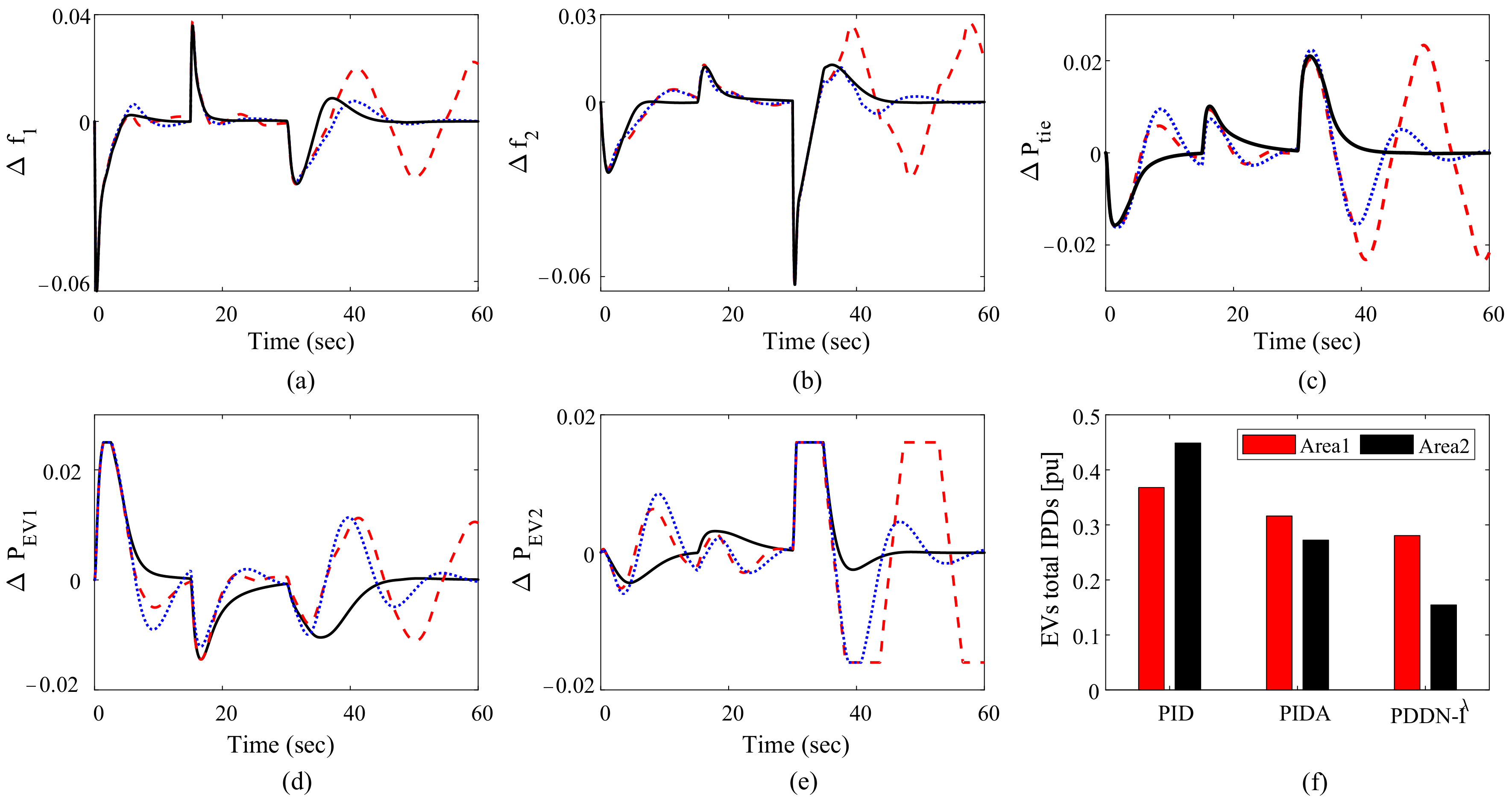
Figure 8.
Dynamic response of the system in case 1: (a) frequency deviations of area 1, (b) frequency deviations of area 2, (c) tie-line power fluctuations, and (d) IPD of the EVs. (e) area 2 EVs ouput, and (f) IPD of the EVs. Solid: Proposed controller, dashed: PID controller, and dotted PIDA.
Figure 8.
Dynamic response of the system in case 1: (a) frequency deviations of area 1, (b) frequency deviations of area 2, (c) tie-line power fluctuations, and (d) IPD of the EVs. (e) area 2 EVs ouput, and (f) IPD of the EVs. Solid: Proposed controller, dashed: PID controller, and dotted PIDA.
Figure 9.
Performance indexes improvements using proposed PDDN-I compared to two other controllers.
Figure 9.
Performance indexes improvements using proposed PDDN-I compared to two other controllers.
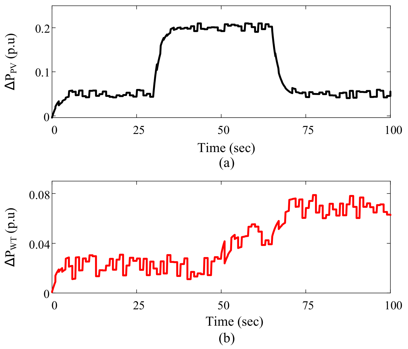
Figure 10.
RESs output power deviations in case 2 (a) PV and (b) WTG.
Figure 10.
RESs output power deviations in case 2 (a) PV and (b) WTG.
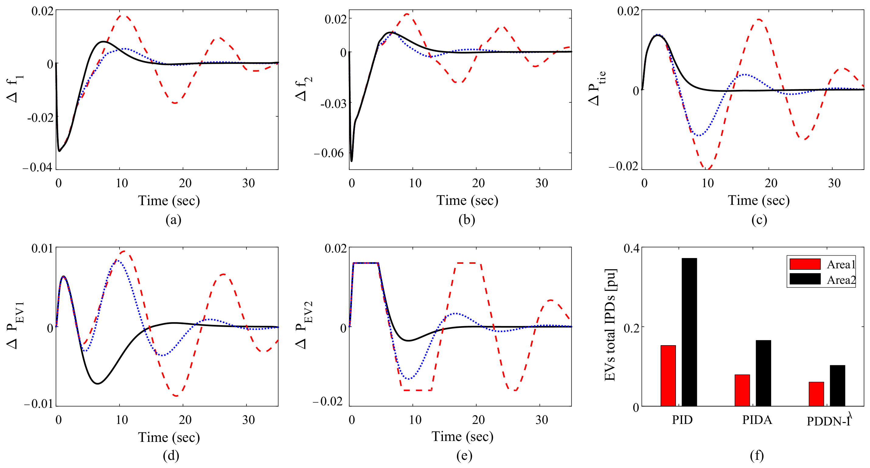
Figure 11.
Dynamic response of the system in Case 2: (a) frequency deviations of area 1, (b) frequency deviations of area 2, (c) tie-line power fluctuations, (d) area 1 EVs ouput, (e) area 2 EVs ouput, and (f) IPD of the EVs. Solid: Proposed controller, dashed: PID controller, and dotted PIDA.
Figure 11.
Dynamic response of the system in Case 2: (a) frequency deviations of area 1, (b) frequency deviations of area 2, (c) tie-line power fluctuations, (d) area 1 EVs ouput, (e) area 2 EVs ouput, and (f) IPD of the EVs. Solid: Proposed controller, dashed: PID controller, and dotted PIDA.
Figure 12.
Dynamic response of the system and IPDs of the EVs in Case 3: (a) frequency deviations of area 1, (b) frequency deviations of area 2, (c) tie-line power fluctuations, (d) area 1 EVs ouput, (e) area 2 EVs ouput, and (f) IPD of the EVs. Solid: Proposed controller, dashed: PID controller, and dotted PIDA.
Figure 13.
Dynamic response of the system in Case 4. (a) frequency deviations of area 1, (b) frequency deviations of area 2, (c) tie-line power fluctuations. Solid: PDDN-I, dotted: PIDA, and dashed: PID controller.
Figure 13.
Dynamic response of the system in Case 4. (a) frequency deviations of area 1, (b) frequency deviations of area 2, (c) tie-line power fluctuations. Solid: PDDN-I, dotted: PIDA, and dashed: PID controller.
Figure 14.
Applied RES’s perturbations to the system in Case V: (a) Load perturbations, (b) PV unit fluctuations, and (c) WTG unit fluctuations.
Figure 14.
Applied RES’s perturbations to the system in Case V: (a) Load perturbations, (b) PV unit fluctuations, and (c) WTG unit fluctuations.
Figure 15.
Dynamic response of the system in Case 5: (a) frequency deviations of area 1, (b) frequency deviations of area 2, (c) tie-line power fluctuations. Solid: PDDN-I, dotted: PIDA, and dashed: PID controller.
Figure 15.
Dynamic response of the system in Case 5: (a) frequency deviations of area 1, (b) frequency deviations of area 2, (c) tie-line power fluctuations. Solid: PDDN-I, dotted: PIDA, and dashed: PID controller.
Figure 16.
Applied disturbances in (a) PV unit, (b) WTG unit, and (c) power demand, in Case 6.
Figure 16.
Applied disturbances in (a) PV unit, (b) WTG unit, and (c) power demand, in Case 6.
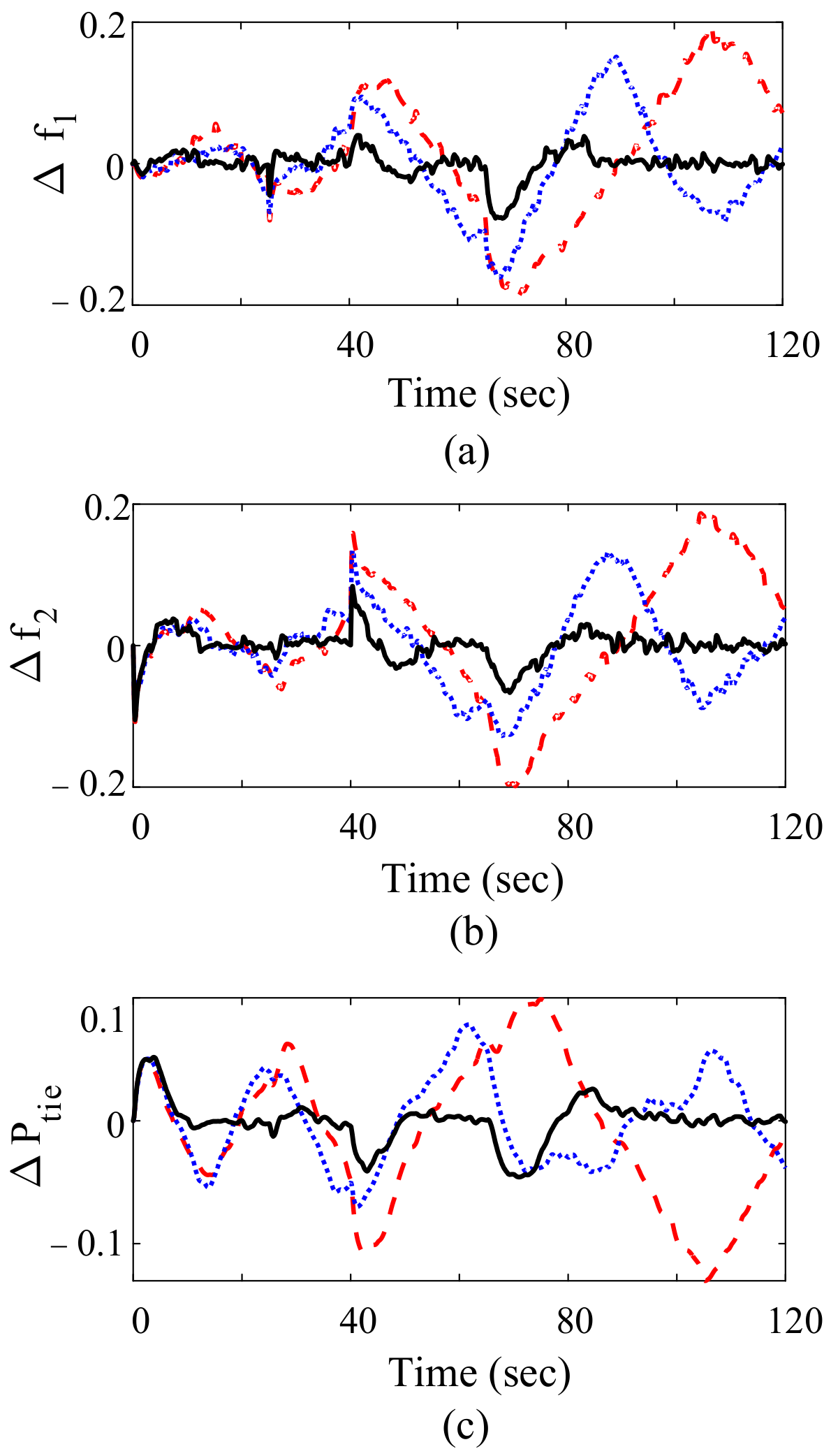
Figure 17.
Dynamic response of the system in Case 6. (a) frequency deviations of area 1, (b) frequency deviations of area 2, (c) tie-line power fluctuations. Solid: PDDN-I, dotted: PIDA, and dashed: PID controller.
Figure 17.
Dynamic response of the system in Case 6. (a) frequency deviations of area 1, (b) frequency deviations of area 2, (c) tie-line power fluctuations. Solid: PDDN-I, dotted: PIDA, and dashed: PID controller.
Figure 18.
Dynamic behavior of the closed-loop test system with different controllers. Solid: Proposed controller, dashed: PID controller, and dashed&dotted: PI Controller.
Figure 18.
Dynamic behavior of the closed-loop test system with different controllers. Solid: Proposed controller, dashed: PID controller, and dashed&dotted: PI Controller.
Figure 19.
System configuration for RCP test.
Figure 19.
System configuration for RCP test.
Figure 20.
Output voltage waveform (capacitor voltage) in closed-loop system with different controllers. (a) PDDN-I, (b) PI, (c) PID, and (d) All-in-one plot using extracted real-time data in MATLAB.
Figure 20.
Output voltage waveform (capacitor voltage) in closed-loop system with different controllers. (a) PDDN-I, (b) PI, (c) PID, and (d) All-in-one plot using extracted real-time data in MATLAB.
Table 1.
Assumptions of system operating conditions in each scenario.
Table 1.
Assumptions of system operating conditions in each scenario.
| Cases | Evaluation Conditions |
|---|
| EVs | Load Changes | M and D Changes | [ms] | and |
|---|
| Design | ✓ | ✓ | ✗ | 20 ms | ✗ |
| Case I | ✓ | ✓ | ✗ | 20 ms | ✗ |
| Case II | ✓ | ✓ | ✗ | 20 ms | ✓ |
| Case III | ✓ | ✓ | ✗ | 20 ms | ✓ |
| Case IV | ✓ | ✓ | ✓ | 60 ms | ✗ |
| Case V | ✓ | ✓ | ✓ | 20 ms | ✗ |
| Case VI | ✗ | ✓ | ✓ | 40 ms | ✓ |
Table 2.
OC values after five-time algorithm execution.
Table 2.
OC values after five-time algorithm execution.
| Algorithm | Index | PDDN-I | PID | PIDA |
|---|
| JAYA | Best | 0.008079 | 0.020552 | 0.009950 |
| Worst | 0.016775 | 0.039585 | 0.091644 |
| Mean | 0.009985 | 0.034585 | 0.015949 |
| PSO | Best | 0.009990 | 0.026790 | 0.010590 |
| Worst | 0.230817 | 0.510817 | 0.329790 |
| Mean | 0.017908 | 0.179790 | 0.067908 |
Table 3.
Optimal parameters of the controllers.
Table 3.
Optimal parameters of the controllers.
| Controller | Control Area | Parameters |
|---|
| PIDN | Area 1 | |
| Area 2 | |
| PIDA | Area 1 | |
| Area 2 | |
| PDDN-I | Area 1 | |
| Area 2 | |
Table 4.
Performance indexes of controllers in different cases.
Table 4.
Performance indexes of controllers in different cases.
| Cases | Controller | Indexes |
|---|
| IAE | ITSE | OC |
|---|
| | PID | 1.6882 | 1.0778 | 55.9232 |
| Case I | PIDA | 0.9419 | 0.3030 | 19.9681 |
| | PDDN-I | 0.7708 | 0.2580 | 15.2861 |
| | PID | 3.1361 | 2.5425 | 109.5704 |
| Case II | PIDA | 5.6585 | 7.1840 | 229.5071 |
| | PDDN-I | 2.7840 | 2.5402 | 104.6916 |
| | PID | 1.0202 | 0.1531 | 12.3856 |
| Case III | PIDA | 0.4561 | 0.0205 | 2.3427 |
| | PDDN-I | 0.3920 | 0.0165 | 1.4971 |
| | PID | 4.1843 | 4.7589 | 107.5937 |
| Case IV | PIDA | 1.7884 | 0.5403 | 25.3235 |
| | PDDN-I | 1.0524 | 0.1792 | 10.4981 |
| | PID | 22.9511 | 189.9002 | 1618.5702 |
| Case V | PIDA | 9.5728 | 33.1450 | 579.6402 |
| | PDDN-I | 3.9377 | 4.5510 | 175.0161 |
| | PID | 4.1843 | 422.5592 | 3036.1002 |
| Case VI | PIDA | 22.0120 | 132.9727 | 1731.7251 |
| | PDDN-I | 3.4430 | 2.4325 | 178.4224 |
Table 5.
Controller optimal parameters for RCP test on first-order system.
Table 5.
Controller optimal parameters for RCP test on first-order system.
| Controller | Parameters | |
|---|
| | | N | |
|---|
| PI | 2 | 3.9 | - | - | - |
| PID | 5 | 5 | 0.0010 | 0.018 | - |
| PDDN-I | 1.3 | 1.12 | 0.9007 | 0.001 | 0.9899 |

 ,
, 


