
Synthetic Infra-Red Image Evaluation Methods by Structural Similarity Index Measures

Department of Aerospace Engineering, Chosun University, Gwangju 61452, Korea
*
Author to whom correspondence should be addressed.
Electronics 2022, 11(20), 3360; https://doi.org/10.3390/electronics11203360
Submission received: 11 September 2022
/
Revised: 6 October 2022
/
Accepted: 13 October 2022
/
Published: 18 October 2022
(This article belongs to the Special Issue Guidance, Navigation, and Fault-Tolerant Control of Autonomous Systems)
Abstract
:For synthetic infra-red (IR) image generation, a new approach using CycleGAN based on the structural similarity index measure (SSIM) is addressed. In this study, how window sizes and weight parameters of SSIM would affect the synthetic IR image constructed by CycleGAN is analyzed. Since it is focused on the acquisition of a more realistic synthetic image, a metric to evaluate similarities between the synthetic IR images generated by the proposed CycleGAN and the real images taken from an actual UAV is also considered. For image similarity evaluations, the power spectrum analysis is considered to observe the extent to which synthetic IR images follow the actual image distribution. Furthermore, the representative t-SNE analysis as a similarity measure is also conducted. Finally, the synthetic IR images generated by the CycleGAN suggested is investigated by the metrics proposed in this paper.
1. Introduction
When performing guided pilot simulations or flight test simulations required for various purposes, the quality of dynamic and synthetic sensor images generated from the sensor models in the given simulation environment is highly important for target recognition, tracking, and behavior for various reconnaissance missions. Due to the fact that testing a modern-guided control system based on such virtual image generation is relatively cost-effective, many relevant studies have been continued consistently. In particular, the generation of synthetic infra-red (IR) images has an important role in evaluating various control algorithms for simulated flight tests, search and reconnaissance missions, and so on. Unfortunately, synthetic IR images generated using numerical methods or algorithms developed so far are still different from actual images [1,2], and it is even difficult and boring to obtain such images in the actual complex environment. It is essential to have real sensor images or very realistic synthetic images in order to evaluate ultra-precise IR image-seeker algorithms. If the difference between the synthetic sensor image and the real sensor image can be analyzed and regenerated properly, it is possible for the synthetic sensor image to replace the actual sensor image. Therefore, the major purpose of this paper is to design an algorithm suitable for generating a more realistic synthetic sensor image and to provide a metric by which the image similarity with actual IR images can be evaluated.
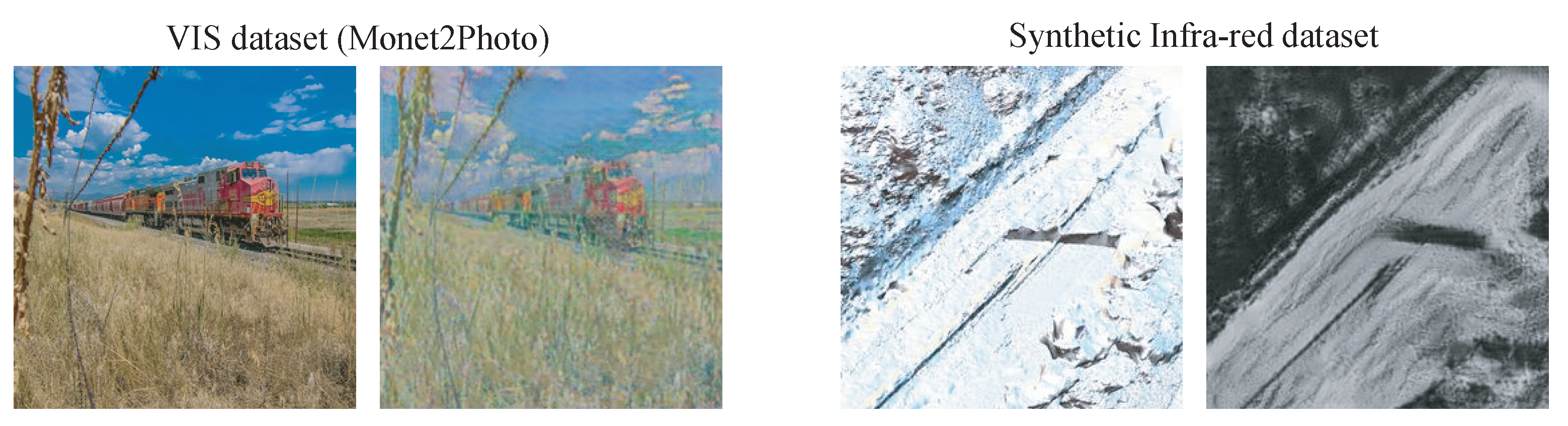
One of the successful techniques for image generation is computer vision based on a convolution neural network (CNN) [3]. It focuses on whether it is possible to learn, classify, and recognize patterns of image data. On the other hand, an exceptional technique using a generative adversarial network (GAN) [4] has been observed for image generation and transformation. GAN is the generative model, where the generator and the discriminator learn adversarial to construct a similar data distribution between latent vectors and the target set. Furthermore, the synthetic image generation close to the target set is possible even in a situation where training data are scarce. However, due to the inherent characteristics of GAN, it is quite hard to adjust constructed synthetic images. DCGAN [5] improves the stability of learning by replacing the non-differentiable part with convolution. DCGAN is divided into two branches; unconditional GAN and conditional GAN. The notable modification in unconditional GAN is PGGAN [6], which detailed functions by gradually building a network layer, and styleGAN [7,8], which enables scale-specific controls in high-resolution images. They reconstructed the structure of the generator by applying the concept of style transfer [9] in the PGGAN. Conditional GAN (cGAN) [10] has been observed to facilitate image adjustments that are difficult in unconditional GAN. Therefore, applications using modified GAN have been observed. Phillip and Isola proposed Pix2pix to learn from paired images [11]. This presented a method of learning by replacing the noise vector of GAN with a sketch figure. This produces improved results in image conversion processes. CycleGAN [12], a type of cGAN, is suitable for this study, and it learns from unpaired data and maps images from one domain to another domain. The loss function used for image generation in the generic CycleGAN proceeds in the direction of minimizing the mean square error (MSE), but it has a limitation in that it cannot catch the details of high-resolution textures, resulting in lower image quality. Many researchers improved the network and loss function of CycleGAN to improve performance [13,14,15,16,17]. In contrast, it is quite difficult (as there is a lack of precedents) and not intuitive to reconstruct a synthetic IR image. As a single example, Figure 1 shows the results of learning the visible (VIS) image and synthetic IR image with CycleGAN. It works well in the VIS domain, but the conversion of the IR image is not good enough. To facilitate image adjustments by humans, the proper index for learning is highly required.
In this study, the structural similarity index measure (SSIM) [18,19] is addressed as a metric to measure the similarity between two images. This is a measure designed to evaluate human visual differences and not numerical errors. It is derived from the fact that human vision is specialized in deriving structural information of images, so the distortion of structural information has a great effect on perception. Thus, by investigating SSIM parameters, a detailed characteristic of this loss function can be observed Some of the literature has succeeded in applying SSIM to the loss function [20,21,22,23]. Therefore, it is believed that applying the SSIM metric to the loss function of CycleGAN can provide a insights in controlling image adjustments. Crossing the two domains CycleGAN creates a synthetic IR image from the virtual image. It is examined in this work how SSIM is applied to loss function to overcome the limitations of traditional network methods.
One of the key issues in this paper is to evaluate output images constructed by each modified GAN. The notable indices that can be quantitative and qualitative evaluation techniques can include the inception score (IS) [24,25,26] and Fréchet inception distance (FID) [27,28]. These methods deeply rely on a pre-existing classifier, that is, InceptionNet, trained on ImageNet. The basic idea of IS is to calculate the Kullback–Leibler divergence between the conditional class distribution and the marginal class distribution over the generated image. However, it is also known that IS is quite sensitive to the prior distribution over labels and the inception models applied. Next, FID computes the Fréchet distance between multivariate Gaussians from the Inception-v3 network. FID has been widely applied to evaluate the performance of GAN due to its consistency with human inspection and sensitivity to small changes in the real distribution. However, as these indices rely on a pre-existing classifier, it is quite difficult to define the similarity for the different class of images, that is, IR images.
In this paper, the similarity between actual IR image sets and synthetic IR images generated by learning is also inspected by defining two indices. A popular method to perform similarity analysis is the t-distributed stochastic neighbor-embedding (t-SNE) technique [29,30,31,32] learning a low-dimensional embedding of the data. That is, each high-dimensional image is represented by a low-dimensional point in such a way that nearby points correspond to similar images and that distant points correspond to dissimilar images. Since the t-SNE technique visualizes the similarity in high-dimensional space in two dimensions, it can be determined that the two data distributions are similarly generated. In this study, real IR images gathered by the actual environment for training, latent vectors extracted from the virtual model, and synthetic IR images generated by CycleGAN are analyzed by using t-SNE. Next, it is also known that the log power spectra of real natural images containing objects with an exponential size distribution are an approximately linear pattern with spatial frequency [33,34,35]. In this study, by analyzing the log power spectrum of the IR actual images and the synthetic image generated by CycleGAN proposed, the similarity between them can be investigated. It is believed that the log power spectra can be a new index to evaluate how similar the synthetic IR image is with the natural IR image.
The main contributions of this paper can be summarized as follows:
- A modified network based on CycleGAN is proposed for realistic synthetic IR image generation by applying the SSIM loss function.
- Various parametric analyses are performed for adjusting synthetic image details generated by the generative model according to the window size and weighting parameters of the SSIM loss.
- The t-SNE and power spectral density (PSD) are proposed as evaluation metrics for image similarity analysis.
This paper is organized as follows. A brief review of GAN is provided in Section 2. The loss function containing the human visual information in this study is addressed, and it is implemented in the CycleGAN proposed. The detailed analysis is conducted according to the change of the weighting parameter and the window size of the SSIM loss function. Next, to demonstrate the effectiveness of SSIM loss on learning by comparing it with the loss, CycleGAN is implemented, particularly in an IR image domain. This process is discussed in Section 3. Then, two techniques, which are t-SNE and power spectra analysis, used as evaluation metrics for the similarity between two images are introduced and applied to the IR images generated by GAN. Implementation results and image evaluation metrics are provided in Section 4. Then, it is concluded in Section 5.
2. Theoretical Background
2.1. Generative Adversarial Network
In this section, let us briefly review the generative adversarial networks. It is well known that one of the AI technologies focusing on the image generation is the GAN. GAN is a generation model that generates fake data close to target images. This trains two different adversarial networks and generates realistic fake data. The problem to be solved in the GAN model is to interpret an image in one domain into another domain. At this time, in the case of a model, such as pix2pix [11], in which the correct answer exists, a pair of images corresponding to both domains must exist in order to be correctly interpreted. However, it is quite hard to construct the datasets. This means that it is difficult to construct the paired image in a real environment.
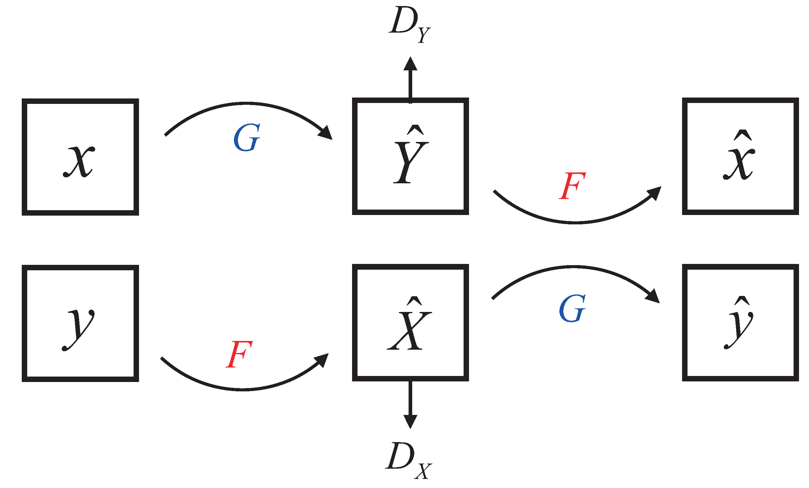
There is an effort on resolving this problem by using the unpaired two image sets. The successful method of resolving this problem can be the CycleGAN approach, which belongs to cGAN and learns with unpaired images. This is a type of unsupervised learning, and the generator learns the image feature of the real image domain rather than learning using correct answers and mapping the image according to their features. In this, two generators illustrated in Figure 2 learn together simultaneously. G function maps from the X domain to the Y domain, F function maps from the Y domain to the X domain, and and are discriminators for each domain X and Y. Each of them learns to deceive the discriminator for the opposite domain. One of the well-known training issues is that if there is no correct answer to image generation, a mode collapse problem may appear in which the model to be trained does not cover the real data distribution and loses diversity. In order to solve this problem, cycle consistency loss [12] was introduced so that domain maintenance can be performed stably. For more consistency, the U-Net [36] structure is utilized as a default framework, and the ResNet [37] structure to the transformer between encoder and decoder is also applied. The residual block can be added to the existing convolution structure since the risk of gradient vanishing/exploding problem is very high as the layer deepens.
2.2. Structural Similarity Index Measure
Structured images have strong correlations between pixels, and these correlations convey visually important information. Error-based image quality evaluation metrics such as MSE and peak signal-to-noise ratio (PSNR) [38] use a linear transformation to calculate an index without including this correlation. The drawback of error-based image quality evaluation metrics is that they often show different results from the human visual system. For these reasons, the structural similarity index measure is considered in this paper. It is a method designed to evaluate human visual differences rather than to only compute numerical errors. By using this approach, the image quality is evaluated with respect to three diimensions: brightness, contrast, and structure. These three factors are derived from the fact that they have the greatest impact on human visual system. Each value is calculated as follows [18,19]:
where , and represent brightness, contrast, and the structure of an image, respectively. , , and are weighting constants to prevent denominators from being zero. It is in general expressed as and , and the nominal values are given by , , and , respectively. Moreover, and denote the mean value and standard deviation defined as follows, respectively:
where N is the total number of pixels, and and are the mean value and the standard deviation of x, respectively. Furthermore, is the covariance between x and y, defined as follows.
Note that . Then, the structural similarity index measure is defined as follows.
2.3. Evaluation Metrics
As mentioned in the Introduction briefly, some studies on how to evaluate the images generated by GAN have been observed. IS evaluates the quality and diversity of generated images using entropy calculation. One of the useful metrics is the FID, which evaluates the image by comparing the real dataset and the generated dataset of the target domain. However, the two techniques are not only difficult to be a quantitative standard metric in image evaluation but also cannot explain the difference between the real image and the fake image perceived by the human visual system. As these evaluation matrices rely on a pre-existing classifier, it is quite difficult to define similarity as a metric between the synthetic images generated by GAN and real images.
Thus, it is necessary to evaluate how close the fake image generated by the GAN is to the real natural image. Thus, data similarity analysis is examined in this paper. Principal component analysis (PCA) [31,39] is basically used to visualize the data vectors. This is a method of analyzing covariance between data to obtain a linear transformation matrix and to reduce the dimension. However, since PCA uses a linear transformation, characteristic extraction is difficult for nonlinear data of high dimensions. Stochastic neighbor embedding (SNE) [40] is a type of dimension-reduction technique that uses a nonlinear method. A similarity of points in a high-dimensional space can be preserved even in a low-dimensional space and learned to minimize the difference between the similarities in order to express the high-dimensional data distribution in a low-dimensional form. By visualizing this, similar data structures in the high-dimensional correspond closely to low-dimensional data structures. This calculates the Euclidean distance and is converted into a conditional probability indicating similarity. Let us assume that x is high-dimensional data, and y is low-dimensional data. Then, the conditional probabilities for x and y are given by the following, respectively.
Furthermore, the distance between points i and j are symmetrically used to solve the crowding problem in which SNE cannot express long distances in higher dimensions as substantially as it can in low dimensions when embedding data utilizes a t-distribution with a larger variance than the normal distribution. Finally, the low-dimension conditional probability of t-SNE [29,30] is expressed as follows.
It is known that this technique provides more stable embedding results than other algorithms for vector visualization. The relationship between the fake image and the real image generated using t-SNE can be identified and used as an evaluation metric in this paper.
Another useful metric for measuring a natural image is the PSD [33,34,35], which is a visualization technique of the spatial frequency of an image using the Fourier transform. This divides the entire time series into short intervals and displays the values obtained by the fast Fourier transform on a logarithmic scale within the mean. The Fourier transform for the image is given by the following:
where u and v are the coordinates of spatial frequency. is the weighted mean intensity defined as follows.
Note that the PSD of natural images tends to have a linear distribution. By inspecting the result of the PSD of the generated image, it is possible to evaluate properly the similarity between real natural images and the fake images generated by GAN. The related studies developed so far on image generation and evaluation are summarized in Table 1.
3. Materials and Method
3.1. CycleGAN Network Architecture
Let us first set up domain A as a virtual environment and domain B as an actual IR environment. Therefore, an image generated using CycleGAN proposed in this study can also be regarded as domain B for this simulation study. One of the main purposes of this study is to generate a synthetic IR image that is much closer to the real IR image. To meet this purpose, the SSIM function is applied to the loss function of CycleGAN by analyzing various deformations.
The proposed architecture of the learning process is explained in detail. The CycleGAN proposed in this study also learns two generators , and discriminators and that can switch between two domains. The generator receives unpaired images of one domain as input and maps them to another domain. At this time, considering that it is unsupervised learning, the cycle consistency loss is added to the adversarial loss to increase the learning stability. Moreover, the generator consists of an encoder, a transformer, and a decoder. Note that the encoder and decoder follow the U-Net structure. The encoder utilizes three convolution layers, and the transformer is based on ResNet 9-block. The decoder consists of three deconvolution layers, and this structure is paired to form two pairs of networks. The 70 × 70 Patch GAN proposed in [12] is also applied to the discriminator. It performs a regional comparison with patches of a specific size instead of the entire image.
3.2. Loss Function for CycleGAN Training
The popular MSE loss function, sometimes called loss, applied to CycleGAN is in general given by the following.
However, in the case of a grayscale image dataset in which the color map consists of a single channel, the generator could not recover the specific characteristics or structures of original features. As it is necessary to change only the domain style while maintaining original image features as much as possible for more realistic image generation, a parameter for the image additionally controllable by the generator is required. To make this possible, SSIM loss, as a feasible option, is augmented to the existing loss of CycleGAN. Therefore, the total loss function for the cycleGAN proposed is given by the following:
where , and are the weighting constants, and the loss functions are expressed as folows:
where is the adversarial loss, and is the cycle consistency loss. When using adversarial loss alone, it is difficult to ensure the proper learning of mapping functions and mode collapse. Therefore, reducing the space of the mapping function is proposed, which is learned to minimize the difference from the original X when reconstructed back to X in the cyclic mapping. is the identity loss introduced to prevent excessive changes in color or mood. , identical with Equation (7) of G and F, instead of x and y, denotes SSIM losses. Note that the statistical characteristics of the image, such as mean and variance, depend on the region of interest (ROI), and the effect of local computation is superior to that of global computations.
It is important to understand the way the human visual system focuses with respect to distinguishing between real IR and fake IR images. It is known that when people look at an image, they focus on parts rather than the overall image. Actually, many people tend to provide a lower quality score for the image with partial distortions. Therefore, it is believed that much-improved image quality can be provided via local-scale image processing rather than overall image or pixel processing. As mentioned in the previous subsection, SSIM basically can make measurements by using convolution operations in units of regions. When comparing images on a region-by-region basis using SSIM, the boundary of the region called window in this work should be first defined. Thus, the pre-defined window determines the region for comparison of the convolution layer. Within the defined window, the mean, standard deviation, and covariance are computed to estimate the brightness, contrast, and structure, respectively. The image metric evaluation by SSIM is conducted based on window size, not pixel-by-pixel, so that the learning is carried out firstly in an 11 × 11 window without considering the viewing condition. Additionally, the multi-window SSIM loss function proposed in this study is expressed as follows:
where is the SSIM loss function with a window size of , and is the weight parameter for each . For the parametric analysis of the multi-scale window size [41], a case for two-windows posessing the sizes of and is examined in this work.
As mentioned before, the human visual system compares brightness, contrast, and structure between two images to figure out the image quality. These values are simply calculated using Equations (1)–(3). However, the three factors can be evaluated differently depending on the human visual system. For a more structural analysis, a new weighting parameter for SSIM is also suggested in this work. The previous statistical values are augmented as follows:
where and are the weight parameters for and in Equations (4)–(6), respectively. It is possible to inspect how the image is changed by controlling each weight parameter in SSIM. The weight parameters are calculated by applying Equation (7).
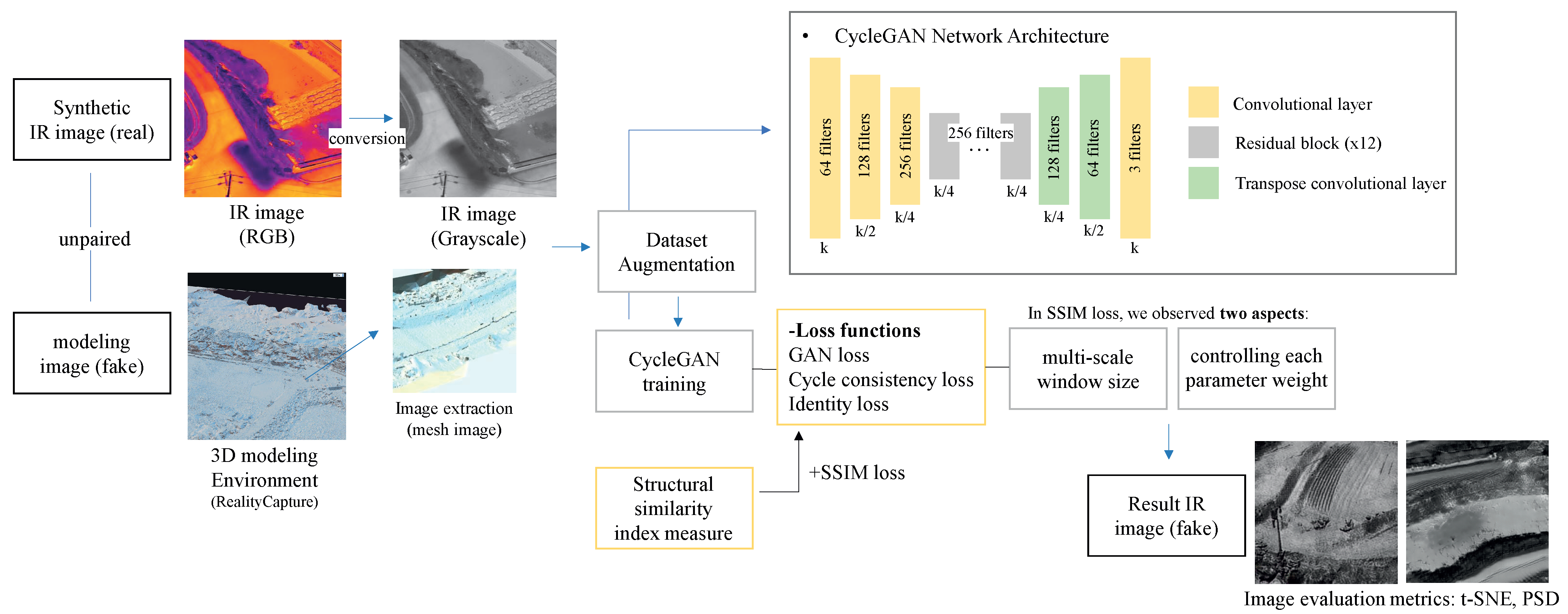
Meanwhile, in most cases, the data for GAN training is obtained based on the visual camera so that temperature deviation cannot be considered. Meanwhile, in the case of IR images, the brightness and structure of the image imply a temperature deviation. It is true by inspecting the actual IR image taken in the real environment. For example, the contrast of IR images is relatively high when the temperature deviation is large. Within the case of information restriction, it is believed that the SSIM suggested can provide much flexibility for IR image generation. In other words, it means that there would be an image change if the weight for each element proposed in this work is adjusted. It will be shown whether different results could be shown for one image by parameter adjustment in the next section. More specifically, image changes can be observed after giving weight variations of the mean, standard deviation, and covariance, respectively. Figure 3 provides a overall methodological flowchart of the research suggested in this paper.
4. Simulation Results
4.1. Dataset and Training Details
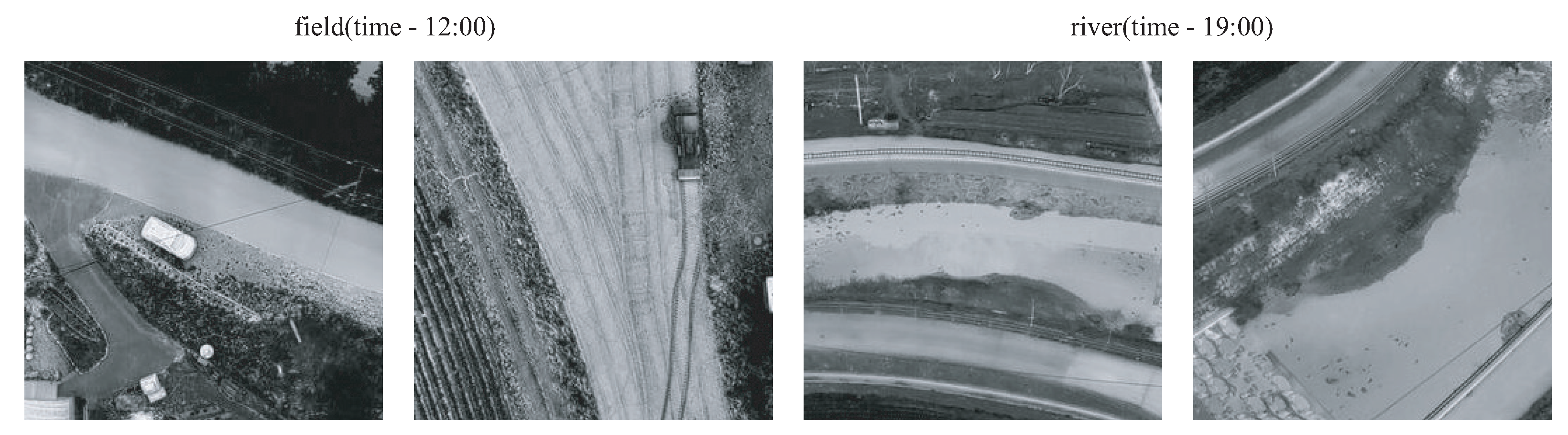
In this section, a numerical simulation study using collected IR images is conducted. Since the dataset for GAN learning requires two different domains, aerial IR images are collected using a drone system equipped with a thermal imaging camera. The specifications of the UAV system and camera used are provided in Table 2 and Table 3. In the experiment, two sets of IR data are collected: a field image taken at 12:00 and an image taken around the small stream at 19:00. In actual implementation, most cases of IR sensors are based on the graycale rather than RGB. Therefore, collected images are converted into the grayscale. Figure 4 shows sample pictures converted to the grayscale from RGB images. In order to build a different domain image that pretends it is generated from a virtual IR environment, 3D modeling by using a commercial software tool was performed from the images taken from the UAV visual camera. Then, from the model, a set of virtual IR images named mesh image in this paper is constructed. At this time, the quantity of image data can be increased by adjusting the contrast and so on. All images are converted to the size of 256 × 256. In addition, for data extension, images rotated 270 degrees are also included in the dataset.
The CycleGAN with the proposed loss function in this study is trained with two NVIDIA GeForce RTX 3090s. The specifications of the learning machine used are provided in Table 4. Total 2480 real field IR images are utilized for the target image set and 940 images are extracted from the virtual model and 1900 IR images to train the network. Next, 430 images are ready for test data. Moreover, a total of 1417 images taken from the small stream dataset are used in this experiment. Images numbering at 659 are extracted from the virtual model, in addition to 812 IR images. Furthermore, 209 images in this case are supposed to be used as the test data.
4.2. Experimental Study
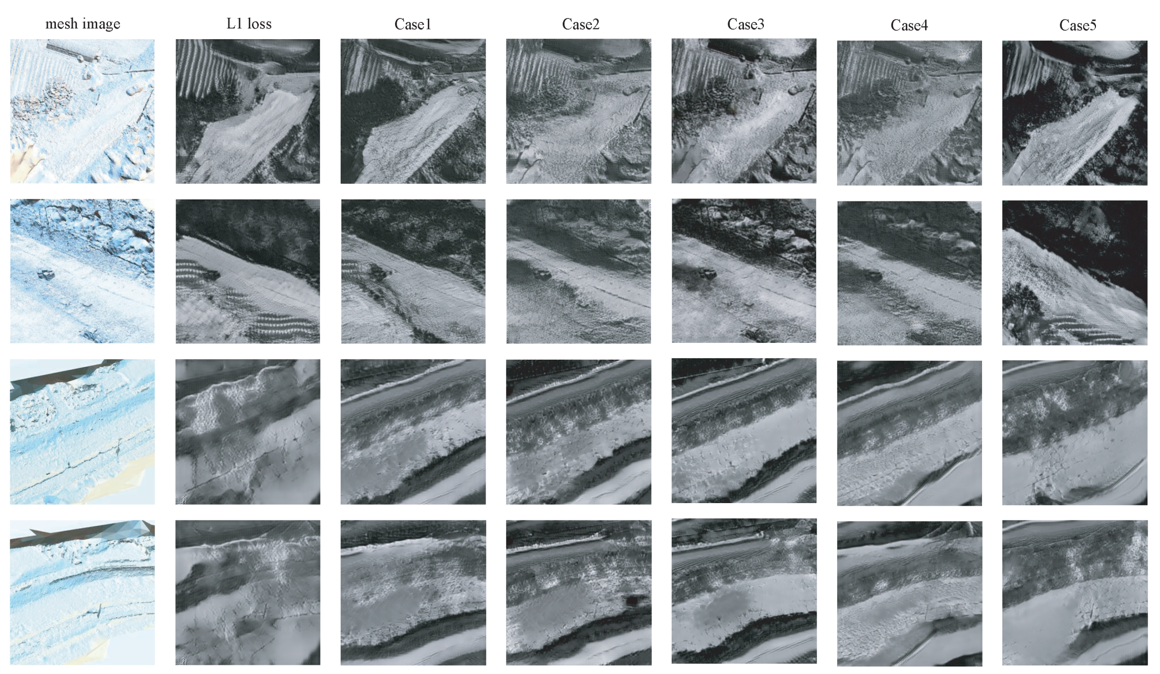
With the collected two domain datasets examined in the previous subsection, the proposed network is trained. The purpose of this study is not only to retain the features of the original image as much as possible but also to change the domain to the realistic IR domain. To evaluate the function of the modified loss function of CycleGAN with respect to the given weight parameters and window size shown in Table 5, several network-learning procedures are performed by adjusting each parameter. Note that , and of Equation (14) are set to 10, 0.1, and 1, respectively. In this study, two different window sizes of and are considered. They operate independently and learns with respect to the weight parameters of the two windows as listed in Table 5. Note that is the weight value for and is the weight values for in Equation (15). For example, Case 1 in Table 5 is only related to the SSIM loss for a single window of , since the weight parameter is determined to be zero. The equally contributed case for the two windows can be Case 3, since the value of weighting parameters is equally chosen. Note that the SSIM loss is calculated as Equation (15) according to the weight for each window. For these case studies, the SSIM parameter weighting parameters of , , and are all chosen as an identical value of 20. Lastly, the proposed synthetic IR image generation network suggested for improving reality is compared with the conventional loss network.
Now, let us inspect the image comparison shown in Figure 5 with respect to window sizes and parameter variations. It is clearly seen in Figure 5 that when only loss is only implemented, images constructed are sometimes damaged and meaningless patterns are generated repeatably, and certain important original features are destroyed. Next, let us examine the remaining cases provided by the suggested method. It is seen that an almost identical image restoration is performed without a loss of the original image feature. According to the window size, the amount of restoration to the original image decreased or increased. Furthermore, it is also revealed in the most cases except the case that the objects in the different domains are not blurred while the domain style of the object is transformed. The image feature (Case 1) with a single window of is rather recovered better than Case 5 of a single , which is the default setting value in this study. Case 3 in which an identical weight value is chosen as 0.5 provides the best image generation without blurring original features.
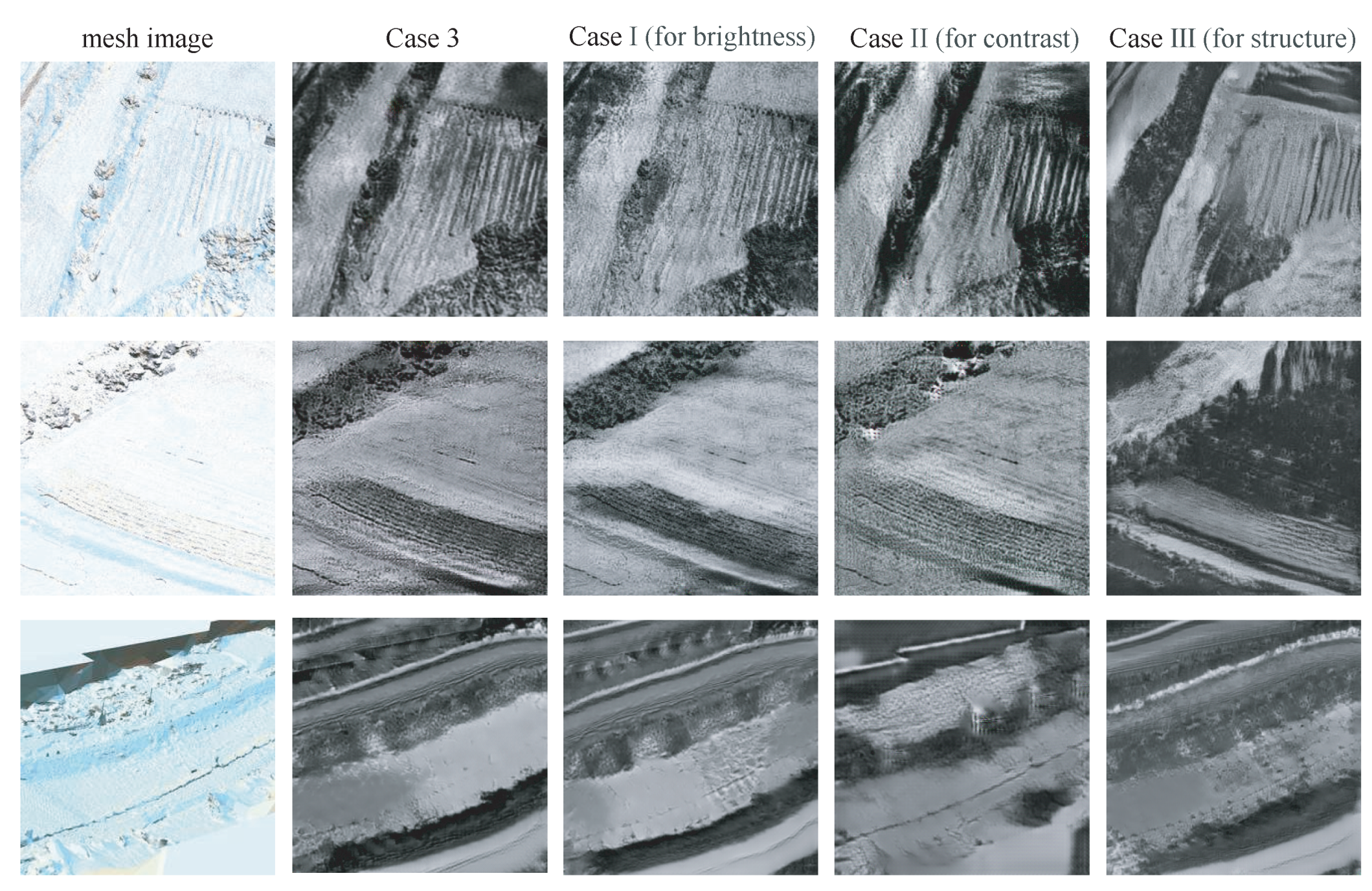
From now on, let us examine the network trained according to the variation of the weight parameters of SSIM for brightness (Case I), contrast (Case II), and structure (Case III). A default sample (Case3) is determined by setting all weighting parameters to an identical value. To highlight the importance of each visual information, it is observed in Table 6 that the weight parameters are assigned dramatically. Case studies are shown in Figure 6. When the weight for brightness increased, for example, the overall brightness of the image generated increased while the contrast and structure features of the image weakened (Case I). Likewise, when the weight related to contrast increased, the contrast of the image clearly increased (Case II). Lastly, when the weight for structure increased, the distortion rate of the image increased (Case III). From these facts, it can concluded that image generation can be controlled by adjusting the weighting parameters of SSIM.
4.3. IR Image Similarity Analysis
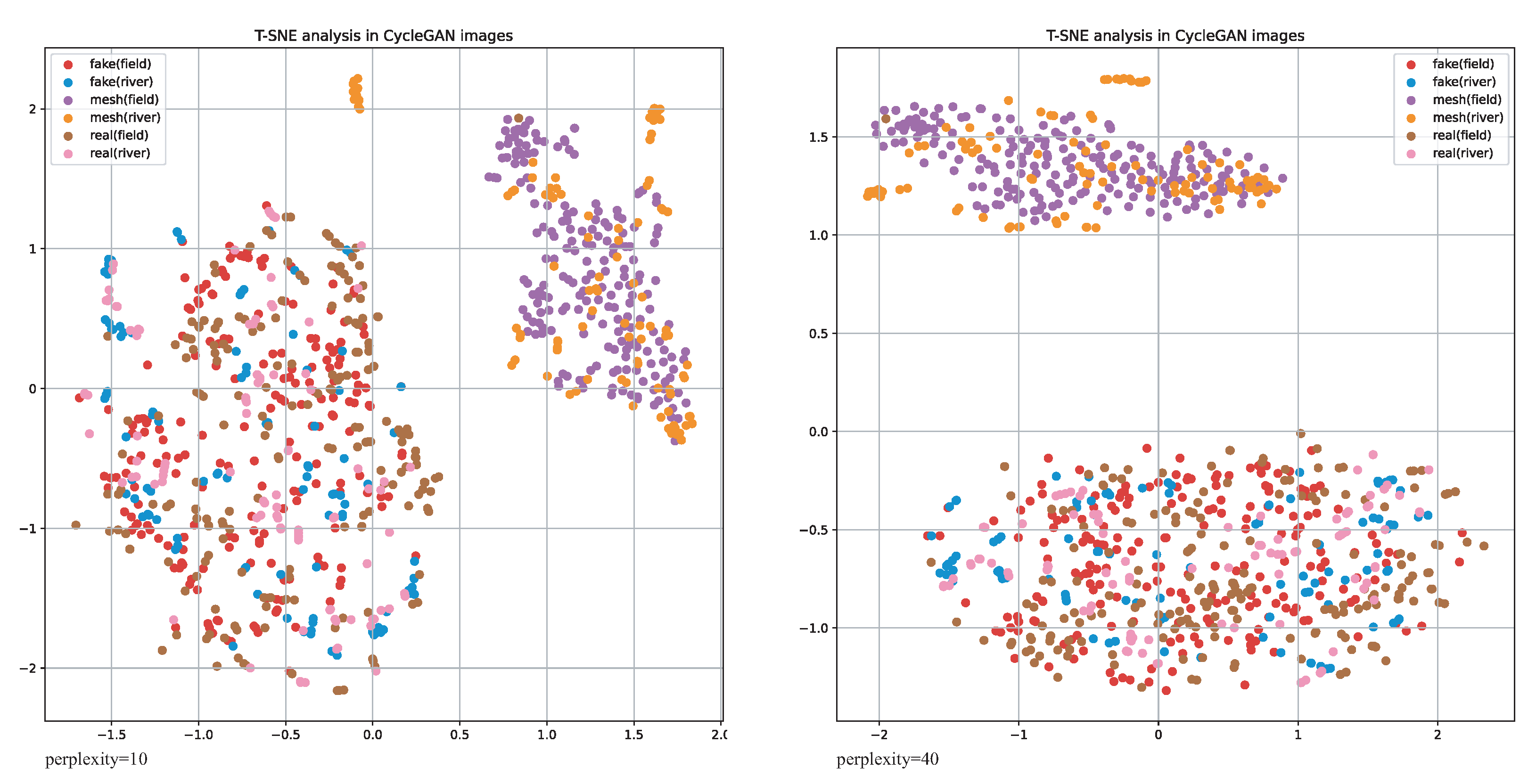
For evaluating the similarity between several images, the t-SNE data visualization technique is applied to three types of IR images inspected in this study. The images are the IR data used for training, the mesh data extracted from the virtual model, and the fake IR data generated by CycleGAN. To visualize the data in a two-dimensional graph, PCA is needed to be subjected to high-dimensional pre-treatment before t-SNE is applied. Figure 7 shows the result of graphs according to the complexity. It is seen that the virtual IR images generated by 3D modeling in the mesh data domain are grouped far from the real IR images. On the other hand, the points representing the real IR image and the synthetic IR fake image generated by the proposed CycleGAN are all scattered together within certain boundaries. Since the t-SNE technique visualizes similarities in high-dimensional space in two dimensions, it can be determined that the two data distributions are very similar.
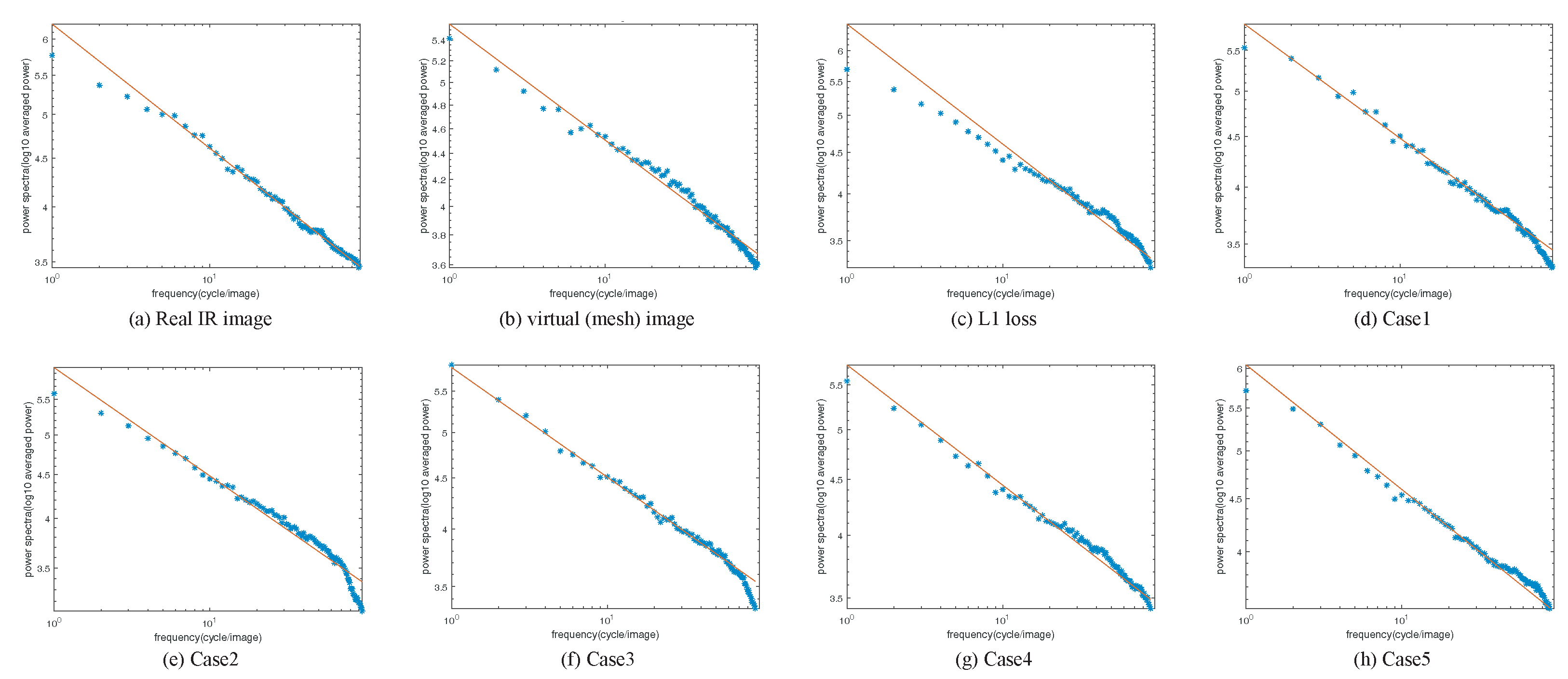
Next, the power spectrum density analysis is applied to various cases simulated in this study. Figure 8 shows the results of power spectrum density for both of the real image and the generated IR images. Figure 8a is of the spectrum for a real IR image. It is seen that the frequency distribution in a log sale of the natural image maintains linearity. Image (b) is an image extracted from the virtual model, and it is seen that the spectrum distribution dropped in the high frequency section. Furthermore, the spectrum is relatively curved. Thus, if the spectrum is similar to (a), it can be regarded that the image is closer to the natural image. That is, if the magnitude of the spectrum does not maintain linearity, it might be regarded as a fake image. The spectrum of (c) is the case of using the loss alone. It is shown that the overall plot of the graph is similar to (b), which is the unnatural case. The spectra of (d)–(h) for the fake images generated are related to the case of using SSIM loss with a variety of weight parameters. It can be concluded that the magnitude of the low-frequency band increased so that the linearity of the graph improved. That is, it is seen that the fake IR image (d)–(h) learned by the SSIM loss complies with the spectral distribution of the actual image rather than the image using the loss of (c).
5. Discussion and Conclusions
Synthetic images generated using various models rely on simple environments rather than specific information. In general, since acquiring an IR image in a complex environment is expensive, technologies for acquiring a synthetic image hvae been studied by composing a 3D target model with software and developing various IR radiation models. However, since the IR synthetic image created by the current generative model is not good enough, a new approach to create IR images that are likely similar to the class of real IR images is addressed by using CycleGAN in this study.
A substantial amount of data are required for good results when training generative model networks. However, it is in general not easy to obtain the IR sensor image required for the network training. In this paper, a technique to generate synthetic IR images using a modified CycleGAN augmented by the structural similarity measure (SSIM) is proposed. The network suggested with the SSIM loss provides much improved performances in synthetic IR image generation, while the existing CycleGAN with loss is not satisfactorily trained. As seen in the previous section, the specific characteristics of the image that disappeared or blurred when using loss were restored when using SSIM loss. The quality of the IR image indicates improved performance when the network is trained with two windows rather than with a single window. Therefore, it provides a clear fact that there is a difference in image generation depending on the window size and weight parameters representing brightness (Case I), contrast (Case II), and structure (Case III) of the SSIM. By controlling the brightness, structure, and contrast parameters of SSIM, it is possible to evaluate these effects on synthetic IR images. It is revealed that these weight variations provide different image generation results. It is observed that contrast and structure are involved in image distortion, and brightness is involved in the domain change with less distortion. Thus, it is expected that more flexible synthetic images are possible by controlling SSIM parameters.
Lastly, the possibility of PSD and t-SNE as image evaluation metrics for similarity analysis between synthetic images and real images was investigated successfully. The PSD analysis for generated images by the proposed network was also performed. It is clearly known from the investigation conducted in this paper when creating a synthetic image that the magnitude of the high-frequency bands tends to be lower than that of the actual image. By conducting numerical experiments using the proposed learning technique, the construction of a realistic synthetic IR image generation was accomplished successfully. In addition, it is believed that two evaluation measures, t-SNE and power spectral density, are very suitable for IR image similarity analysis.
Author Contributions
Conceptualization, S.H.L. and H.L.; methodology, S.H.L. and H.L.; software, S.H.L.; validation, S.H.L. and H.L.; formal analysis, S.H.L.; investigation, H.L.; resources, S.H.L. and H.L.; data curation, S.H.L.; writing—original draft preparation, S.H.L.; writing—review and editing, H.L.; visualization, S.H.L.; supervision, H.L.; project administration, H.L.; funding acquisition, H.L. All authors have read and agreed to the published version of the manuscript.
Funding
This work was supported by AI based Flight Control Research Laboratory funded by Defense Acquisition Program Administration under Grant UD200045CD.
Data Availability Statement
No new data were created or analyzed in this study. Data sharing is not applicable to this article.
Conflicts of Interest
The authors declare no conflict of interest.
Abbreviations
| 3D | Three-dimensional |
| AI | Artificial intelligence |
| cGAN | Conditional generative adversarial network |
| FID | Fréchet inception distance |
| CNN | Convolution neural network |
| GAN | Generative adversarial network |
| IR | Infra-red |
| IS | Inception score |
| MSE | Mean square error |
| PCA | Principal component analysis |
| PSD | Power spectrum density |
| PSNR | Peak signal-to-noise ratio |
| ROI | Region of Interest |
| SNE | Stochastic neighbor embedding |
| SSIM | Structural similarity index measure |
| t-SNE | t-distributed stochastic neighbor embedding |
| VIS | Visible |
References
- Zhang, R.; Mu, C.; Xu, M.; Xu, L.; Shi, Q.; Wang, J. Synthetic IR image refinement using adversarial learning with bidirectional mappings. IEEE Access 2019, 7, 153734–153750. [Google Scholar] [CrossRef]
- Kniaz, V.V.; Gorbatsevich, V.S.; Mizginov, V.A. Thermalnet: A deep convolutional network for synthetic thermal image generation. Int. Arch. Photogramm. Remote. Sens. Spat. Inf. Sci. 2017, 42, 41. [Google Scholar] [CrossRef] [Green Version]
- Krizhevsky, A.; Sutskever, I.; Hinton, G.E. ImageNet Classification with Deep Convolutional Neural Networks. Adv. Neural Inf. Process. Syst. 2012, 25, 84–90. [Google Scholar] [CrossRef] [Green Version]
- Goodfellow, I.J.; Pouget-Abadie, J.; Mirza, M.; Xu, B.; Warde-Farley, D.; Ozair, S.; Courville, A.; Bengio, Y. Generative adversarial networks. arXiv 2014, arXiv:1406.2661. [Google Scholar] [CrossRef]
- Radford, A.; Metz, L.; Chintala, S. Unsupervised representation learning with deep convolutional generative adversarial networks. arXiv 2015, arXiv:1511.06434. [Google Scholar]
- Karras, T.; Aila, T.; Laine, S.; Lehtinen, J. Progressive growing of gans for improved quality, stability, and variation. arXiv 2017, arXiv:1710.10196. [Google Scholar]
- Karras, T.; Laine, S.; Aila, T. A style-based generator architecture for generative adversarial networks. In Proceedings of the IEEE/CVF Conference on Computer Vision and Pattern Recognition, Long Beach, CA, USA, 16–20 June 2019; pp. 4401–4410. [Google Scholar]
- Karras, T.; Aittala, M.; Hellsten, J.; Laine, S.; Lehtinen, J.; Aila, T. Training generative adversarial networks with limited data. In Proceedings of the IEEE/CVF Conference on Computer Vision and Pattern Recognition, Seattle, WA, USA, 13–19 June 2020; Volume 33, pp. 12104–12114. [Google Scholar]
- Huang, X.; Belongie, S. Arbitrary style transfer in real-time with adaptive instance normalization. In Proceedings of the IEEE International Conference on Computer Vision, Venice, Italy, 22–29 October 2017; pp. 1501–1510. [Google Scholar]
- Mirza, M.; Osindero, S. Conditional Generative Adversarial Nets. arXiv 2014, arXiv:1411.1784. [Google Scholar]
- Phillip, I.; Jun-Yan, Z.; Tinghui, Z.; Alexei, A.E. Image-to-Image Translation with Conditional Adversarial Networks. In Proceedings of the IEEE Conference on Computer Vision and Pattern Recognition, Honolulu, HI, USA, 21–26 July 2017; pp. 1125–1134. [Google Scholar]
- Zhu, J.-Y.; Park, T.; Isola, P.; Efros, A.A. Unpaired Image-to-Image Translation using Cycle-Consistent Adversarial Networks. In Proceedings of the IEEE International Conference on Computer Vision, Venice, Italy, 22–29 October 2017; pp. 2223–2232. [Google Scholar]
- Li, W.; Wang, J. Residual learning of cycle-GAN for seismic data denoising. IEEE Access 2021, 9, 11585–11597. [Google Scholar] [CrossRef]
- Maniyath, S.R.; Vijayakumar, K.; Singh, L.S.; Sudhir, K.; Olabiyisi, T. Learning-based approach to underwater image dehazing using CycleGAN. IEEE Access 2021, 14, 1–11. [Google Scholar] [CrossRef]
- Engin, D.; Genç, A.; Kemal Ekenel, H. Cycle-dehaze: Enhanced cyclegan for single image dehazing. In Proceedings of the IEEE Conference on Computer Vision and Pattern Recognition Workshops, Salt Lake City, UT, USA, 18–22 June 2018; pp. 825–833. [Google Scholar]
- Teng, L.; Fu, Z.; Yao, Y. Interactive translation in echocardiography training system with enhanced cycle-GAN. IEEE Access 2020, 8, 106147–106156. [Google Scholar] [CrossRef]
- Hammami, M.; Friboulet, D.; Kéchichian, R. Cycle GAN-based data augmentation for multi-organ detection in CT images via Yolo. In Proceedings of the 2020 IEEE International Conference on Image Processing (ICIP), Negombo, Sri Lanka, 6–8 March 2020; pp. 390–393. [Google Scholar]
- Wang, Z.; Bovik, A.C.; Sheikh, H.R.; Simoncelli, E.P. Image quality assessment: From error visibility to structural similarity. IEEE Trans. Image Process. 2004, 13, 600–612. [Google Scholar] [CrossRef] [PubMed] [Green Version]
- Zhao, H.; Gallo, O.; Frosio, I.; Kautz, J. Loss Functions for Image Restoration With Neural Networks. IEEE Trans. Comp. Imaging 2016, 3, 47–57. [Google Scholar] [CrossRef]
- Hwang, J.; Yu, C.; Shin, Y. SAR-to-optical image translation using SSIM and perceptual loss based cycle-consistent GAN. In Proceedings of the IEEE Conference on Computer Vision and Pattern Recognition Workshops, Seattle, WA, USA, 14–19 June 2020; pp. 191–194. [Google Scholar]
- Tao, L.; Zhu, C.; Xiang, G.; Li, Y.; Jia, H.; Xie, X. LLCNN: A convolutional neural network for low-light image enhancement. In Proceedings of the 2017 IEEE Visual Communications and Image Processing (VCIP), St. Petersburg, FL, USA, 10–13 December 2017; pp. 1–4. [Google Scholar]
- Shi, H.; Wang, L.; Zheng, N.; Hua, G.; Tang, W. Loss functions for pose guided person image generation. Pattern Recognit. 2022, 122, 108351. [Google Scholar] [CrossRef]
- Yu, J.; Wu, B. Attention and hybrid loss guided deep learning for consecutively missing seismic data reconstruction. IEEE Trans. Geosci. Remote Sens. 2021, 60, 1–8. [Google Scholar] [CrossRef]
- Salimans, T.; Goodfellow, I.; Zaremba, W.; Cheung, V.; Radford, A.; Chen, X. Improved techniques for training gans. Adv. Neural Inf. Process. Syst. 2016, 29, 2234–2242. [Google Scholar]
- Brock, A.; Donahue, J.; Simonyan, K. Large scale GAN training for high fidelity natural image synthesis. arXiv 2018, arXiv:1809.11096. [Google Scholar]
- Barratt, S.; Sharma, R. Robust Backstepping Control of Robotic Systems Using Neural Networks. arXiv 2018, arXiv:1801.01973. [Google Scholar]
- Martin, H.; Hubert, R.; Thomas, U.; Bernhard, N.; Sepp, H. Gans trained by a two time-scale update rule converge to a local nash equilibrium. Adv. Neural Inf. Process. Syst. 2017, 30, 6626–6637. [Google Scholar]
- Obukhov, A.; Krasnyanskiy, M. Quality assessment method for GAN based on modified metrics inception score and Fréchet inception distance. In Proceedings of the Computational Methods in Systems and Software, Online, 14–17 October 2020; pp. 102–114. [Google Scholar]
- Van der Maaten, L.; Hinton, G. Visualizing data using t-SNE. J. Mach. Learn. Res. 2008, 9, 2579–2695. [Google Scholar]
- Van Der Maaten, L. Accelerating t-SNE using tree-based algorithms. J. Mach. Learn. Res. 2014, 15, 3221–3245. [Google Scholar]
- Anowar, F.; Sadaoui, S.; Selim, B. Conceptual and empirical comparison of dimensionality reduction algorithms (pca, kpca, lda, mds, svd, lle, isomap, le, ica, t-sne). Comput. Sci. Rev. 2021, 40, 100378. [Google Scholar] [CrossRef]
- Spiwok, V.; Kříž, P. Time-lagged t-distributed stochastic neighbor embedding (t-SNE) of molecular simulation trajectories. Front. Mol. Biosci. 2020, 7, 132. [Google Scholar] [CrossRef] [PubMed]
- Van der Schaaf, A.; van Hateren, J.H. Modelling the Power Spectra of Natural Images: Statistics and Information. Vision Res. 1996, 36, 2759–2770. [Google Scholar] [CrossRef] [Green Version]
- Koch, M.; Denzler, J.; Redies, C. 1/f2 Characteristics and isotropy in the fourier power spectra of visual art, cartoons, comics, mangas, and different categories of photographs. PLoS ONE 2010, 5, e12268. [Google Scholar] [CrossRef]
- Pamplona, D.; Triesch, J.; Rothkopf, C.A. Power spectra of the natural input to the visual system. Vision Res. 2013, 83, 66–75. [Google Scholar] [CrossRef] [Green Version]
- Ronneberger, O.; Fischer, P.; Brox, T. U-Net: Convolutional Networks for Biomedical Image Segmentation. In Proceedings of the International Conference on Medical Image Computing and Computer-Assisted Intervention, Munich, Germany, 5–9 October 2015; pp. 234–241. [Google Scholar]
- He, K.; Zhang, X.; Sun, J. Deep Residual Learning for Image Recognition. In Proceedings of the IEEE Conference on Computer Vision and Pattern Recognition, Las Vegas, NV, USA, 27–30 June 2016; pp. 770–778. [Google Scholar]
- Hore, A.; Ziou, D. Image quality metrics: PSNR vs. SSIM. In Proceedings of the 2010 20th International Conference on Pattern Recognition, Washington, DC, USA, 23–26 August 2010; pp. 2366–2369. [Google Scholar]
- Jolliffe, I.T.; Cadima, J. Principal component analysis: A review and recent developments. R. Soc. Publ. 2016, 374, 20150202. [Google Scholar] [CrossRef]
- Hinton, G.E.; Roweis, S. Stochastic neighbor embedding. Adv. Neural Inf. Process. Syst. 2002, 15, 749–756. [Google Scholar]
- Wang, Z.; Simoncelli, E.P.; Bovik, A.C. Multiscale structural similarity for image quality assessment. In Proceedings of the Thrity-Seventh Asilomar Conference on Signals, Systems & Computers, Pacific Grove, CA, USA, 9–12 November 2003; Volume 2, pp. 1398–1402. [Google Scholar]
Figure 1.
A single example of learning general dataset (Monet2Photo) and synthetic infra-red dataset. Compared to the VIS data, synthetic IR data were not learned well.
Figure 1.
A single example of learning general dataset (Monet2Photo) and synthetic infra-red dataset. Compared to the VIS data, synthetic IR data were not learned well.

Figure 2.
CycleGAN network diagram.

Figure 3.
Flowchart to illustrate the methodological steps of the study.

Figure 4.
Real IR images taken with a drone system with IR camera (ZENMUSE H20T): the left two images were taken in the field at 12:00, and the right two images were taken around small stream at 19:00.
Figure 4.
Real IR images taken with a drone system with IR camera (ZENMUSE H20T): the left two images were taken in the field at 12:00, and the right two images were taken around small stream at 19:00.

Figure 5.
Constructed image comparison due to multi-window weighting parameters.

Figure 6.
Image construction with respect to the variation of SSIM weight parameters.

Figure 7.
t-SNE analysis for various types of IR images, including the images generated by CycleGAN proposed.
Figure 7.
t-SNE analysis for various types of IR images, including the images generated by CycleGAN proposed.

Figure 8.
Power spectrum analysis for the constructed image by CycleGAN proposed and a natural IR image.
Figure 8.
Power spectrum analysis for the constructed image by CycleGAN proposed and a natural IR image.


Table 1.
The previous literature for image generation and evaluation techniques.
| Items | References | Year of Publish | Description |
|---|---|---|---|
| Generative adversarial network | [4] | 2014 | Generator and discriminator learn adversarial and estimate generative models |
| [11] | 2017 | Image-to-Image translation, adding traditional loss () to improve image quality using conditional GAN | |
| [12] | 2017 | Transformation between unpaired images using cGAN, adding cycle consistency loss to cover the real data distribution | |
| Image quality evaluation metrics | [38] | 2010 | Information on loss of quality of images generated or compressed with a signal-to-noise ratio |
| [18] | 2004 | A method designed to evaluate human visual quality differences and not numerical errors | |
| Image evaluation metrics | [24] | 2016 | GAN performance evaluation in terms of sharpness and diversity |
| [27] | 2017 | The image evaluation by comparing the real dataset and the generated dataset of the target domain | |
| [29] | 2008 | Similarity visualization in high-dimensional space in two dimensions via low-dimensional embedding learning | |
| [33] | 1996 | Visualization technique of the spatial frequency of an image using the Fourier transform |
Table 2.
UAV specification.
| Attribute | Value |
|---|---|
| Description | DJI MATRICE 300 RTK |
| Weight | 6.3 kg (Including two TB60 batteries) |
| Diagonal length | 895 mm |
Table 3.
Camera specification.
| Attribute | Camera Specification |
|---|---|
| Description | DJI ZENMUSE H20T |
| Sensor | Vanadium Oxide (VOx) microwave bolometer |
| Lens | DFOV: 40.6 |
| Focal length: 13.5 mm | |
| Aperture: f/1.0 | |
| Focus: 5 m∼∞ |
Table 4.
Training machine specification.
| Attribute | Training Machine Specification |
|---|---|
| CPU | 1 × Intel i9 X-series Processor |
| GPU | 2 × NVIDIA RTX 3090 (24 GB) |
| Mem. | 192 GB |
Table 5.
Weight parameters in different cases of window size.
| Weight Parameter | Case 1 | Case 2 | Case 3 | Case 4 | Case 5 |
|---|---|---|---|---|---|
| 1.0 | 0.6 | 0.5 | 0.4 | 0.0 | |
| 0.0 | 0.4 | 0.5 | 0.6 | 1.0 |
Table 6.
Weight parameters for the brightness, contrast, and structure of SSIM.
| Weight Parameter | Case I (for Brightness) | Case II (for Contrast) | Case III (for Structure) |
|---|---|---|---|
| 20 | 1 | 1 | |
| 1 | 20 | 1 | |
| 1 | 1 | 20 |
Publisher’s Note: MDPI stays neutral with regard to jurisdictional claims in published maps and institutional affiliations. |
© 2022 by the authors. Licensee MDPI, Basel, Switzerland. This article is an open access article distributed under the terms and conditions of the Creative Commons Attribution (CC BY) license (https://creativecommons.org/licenses/by/4.0/).
Share and Cite
MDPI and ACS Style
Lee, S.H.; Leeghim, H. Synthetic Infra-Red Image Evaluation Methods by Structural Similarity Index Measures. Electronics 2022, 11, 3360. https://doi.org/10.3390/electronics11203360
AMA Style
Lee SH, Leeghim H. Synthetic Infra-Red Image Evaluation Methods by Structural Similarity Index Measures. Electronics. 2022; 11(20):3360. https://doi.org/10.3390/electronics11203360
Chicago/Turabian StyleLee, Sky H., and Henzeh Leeghim. 2022. "Synthetic Infra-Red Image Evaluation Methods by Structural Similarity Index Measures" Electronics 11, no. 20: 3360. https://doi.org/10.3390/electronics11203360
Note that from the first issue of 2016, this journal uses article numbers instead of page numbers. See further details here.