Leveraging a Heterogeneous Ensemble Learning for Outcome-Based Predictive Monitoring Using Business Process Event Logs

Abstract

Outcome-based predictive process monitoring concerns predicting the outcome of a running process case using historical events stored as so-called process event logs. This prediction problem has been approached using different learning models in the literature. Ensemble learners have been shown to be particularly effective in outcome-based business process predictive monitoring, even when compared with learners exploiting complex deep learning architectures. However, the ensemble learners that have been used in the literature rely on weak base learners, such as decision trees. In this article, an advanced stacking ensemble technique for outcome-based predictive monitoring is introduced. The proposed stacking ensemble employs strong learners as base classifiers, i.e., other ensembles. More specifically, we consider stacking of random forests, extreme gradient boosting machines, and gradient boosting machines to train a process outcome prediction model. We evaluate the proposed approach using publicly available event logs. The results show that the proposed model is a promising approach for the outcome-based prediction task. We extensively compare the performance differences among the proposed methods and the base strong learners, using also statistical tests to prove the generalizability of the results obtained.

1. Introduction

Business process monitoring is concerned with extracting previously unknown and valuable insights about business processes from historical data, usually available as so-called event logs [1]. Event logs contain events. Each event is characterized by information regarding the process execution to which it belongs, a.k.a. process case, the activity that was executed, a timestamp capturing the time instant at which an activity was executed, and other domain-specific attributes, such as the human resource that executed the activity. We refer to the sequence of events belonging to the process case as a trace. For instance, in a process about granting building permits by a public administration, a trace collects the events regarding the processing of one specific building permit application.

Predictive process monitoring of business processes has emerged in the last ten years and aims at extracting insights about business processes by building predictive models using event log data [2]. There are several aspects of a process that can be predicted, such as the timestamp of next events [3], the future activities that will be executed in a process case [4,5,6], or the outcome of a process case [7]. Predictive monitoring enables proactive decision making, such as informing customers that their request may be processed later than expected or addressing the possible occurrence of an unfavorable exception by implementing protective measures.

Predictive process monitoring models are developed using classification and regression techniques. Predicting future activities in a case or the outcome of process cases entail the use of classification techniques, whereas predicting timestamps requires regression techniques. In this paper, we focus on outcome-based predictive monitoring, where normally the aim is to predict a binary label capturing the outcome of process cases, e.g., positive vs. negative or regular vs. deviant.

The research on process-outcome-based predictive monitoring has evolved along two main lines. On the one hand, recently, one objective has been to devise more advanced features that can improve the predictive power of the models. Examples are features capturing the load level of the system in which business processes are executed [8] or features capturing the experience of the human resources involved in a process [9]. On the other hand, the objective of researchers historically has been to develop more accurate predictive models. Classifier ensembles have demonstrated some advantages over individual classifiers when they are used in outcome-based predictive monitoring. Teinemaa et al. [7] have reported that XGB emerged as the best overall performer in over 50% of datasets considered in their extensive benchmark. However, its success is assessed in the benchmark against a restricted alternative ensemble architecture.

In this paper, we leverage an advanced heterogeneous ensemble learning method for outcome-based predictive process monitoring. Specifically, we propose to adopt a stacking ensemble technique involving strong learners [10]. In many classification problems, in fact, only weak classifiers such as decision trees or feed-forward neural networks are chosen as base classifiers. Rather than utilizing a weak classifier, we consider in this paper the potential of constructing a classifier ensemble using strong learners. We build an ensemble scheme based on the stacking algorithm, where the base learners are other ensemble learners, i.e., extreme gradient boosting machine (XGB), random forest (RF), and gradient boosting machine (GBM). While XGB and RF have been considered already in previous benchmarks on outcome-based predictive monitoring, GBM has not been considered by previous research in this particular classification problem.

We carried out an extensive experiment considering 25 event log datasets publicly available. Moreover, to provide a fair assessment, we consider an extensive set of performance measures—i.e., F1, F2, MCC, accuracy, area under ROC curve (AUC), and area under precision recall (AUCPR) indices—and use statistical tests to assess the significance of the performance levels and rankings obtained in the experiment. The results show that the proposed model generally outperforms the baselines, i.e., the strong learners used as base models for the ensemble. The performance difference is significant, particularly when considering measures that are more appropriate for imbalanced datasets, such as MCC and AUCPR. Note, in fact, that most outcome labels in most publicly available real-world event logs are strongly imbalanced.

The paper is organized as follows. Section 2 discusses the related work. Section 3 formally defines the problem of outcome-based predictive process monitoring and introduces the stacked ensemble learning method to address it. The evaluation of the proposed method is presented in Section 4 and conclusions are drawn in Section 5.

2. Related Work

Di Francescomarino et al. [11] provided a qualitative value-driven analysis of various predictive process monitoring techniques to assist decision-makers in selecting the best predictive technique for a given task. The review presented by Marquez-Chamorro et al. [2] considers standard criteria for classifying predictive monitoring approaches in the literature, such as the prediction task or technique used. Furthermore, it categorizes approaches in the literature based on their process-awareness, i.e., whether or not an approach employs an explicit representation of process models. Santoso [12] specified a language for properly defining the prediction task, enabling researchers to express various types of predictive monitoring problems while not relying on any particular machine learning techniques.

As far as outcome-oriented predictive monitoring is concerned, Teinemaa et al. [7] developed a comprehensive analysis and quantitative benchmark of different encoding techniques and models using real-world event logs. In this benchmark, RF and XGB are the only ensemble models considered. XGB emerges as the top-performing classifier in the majority of the prediction tasks.

Verenich et al. [13] proposed a transparent approach for predicting quantitative performance indicators of business process performance. The predicted indicators could be more explainable since they were decomposed into elementary components. The explainability of process outcome predictions was addressed recently by Galanti et al. [14] using the SHAP method.

Recently, researchers have increasingly focused on applying deep learning techniques to solve the problem of process outcome prediction. Rama-Maneiro et al. [15] provided a systematic literature review of deep learning techniques for predictive monitoring of business process, discussing an in-depth analysis and experimental evaluation of 10 approaches involving 12 event log datasets. Similarly, in Neu et al. [16], a systematic literature review was carried out to capture the state-of-the-art deep learning methods for process prediction. The literature is classified along the dimensions of neural network type, prediction type, input features, and encoding methods.

Kratsch et al. [17] compared the performance of deep learning, e.g., feed forward neural networks and LSTM networks, and machine learning algorithms, i.e., random forests and support vector machines using five publicly available event logs. Metzger et al. [18] proposed an ensemble of deep learning models that can produce outcome predictions at arbitrary points during process executions. Wang et al. [19] proposed a real-time, outcome-oriented predictive process monitoring method based on bidirectional LSTM networks and attention mechanisms. Better performance could be achieved as the features having a decisive effect on the outcome were identified and optimized.

To address the issue of inaccurate or overfitting prediction models, a fine-tuned deep neural network that learns general-enough trace representations from unlabeled log traces was proposed in [20]. Pasquadibisceglie et al. [21] leveraged a convolutional neural network (CNN) architecture to classify the outcome of an ongoing trace, showing that the proposed technique could be integrated as an intelligent assistant to support sales agents in their negotiations.

Generally, the deep learning approaches in the literature do not always necessarily outscore other more traditional techniques, such as ensembles (e.g., XGB and RF). Therefore, devising novel architectures based on such traditional techniques is still relevant in this prediction context, in particular, to avoid the high training costs (time and computational resources) of deep-learning-based architectures.

3. Problem Definition and Method

In this section, we first formalize the problem of outcome-based process predictive monitoring. Then, we present in detail the proposed stacking ensemble method using strong learners.

3.1. Problem Definition

In an event log, a trace represents the sequence of events recorded during the execution of a business process instance (i.e., a case). Each event in a trace records the information about a specific activity that occurs during the execution of a process case.

We denote the collection of all event identifiers (event universe) by $\mathcal{E}$ and the universe of attribute names by $\mathcal{A}$. An event e is a tuple $e=\langle (c,a,t(d_1,v_1),\dots ,(d_m,v_m)\rangle )$, where c is the case id; a is the activity recorded by this event; t is the timestamp at which the event has been recorded; and $(d_1,v_1),\dots ,(d_m,v_m)$, with $m\ge 0$, are other domain-specific attributes and their values. For instance, the event $e=(5,check,2022.1.2,resource=Alice,amount$ $=1000,type=eligibility)$ captures the fact that, in a process case associated with loan request number 5, the human resource Alice has executed an eligibility check of a loan request of 1000 USD on 2 January 2022. The value of attribute $d_m$ of an event e is denoted by the symbol ${\#}_m\left(e\right)$. The timestamp of the event e, for example, can be represented as ${\#}_t\left(e\right)$. Whenever an event e does not have a value for an attribute $d_i$, we write $v_i=\perp$ (where ⊥ is the undefined value). For instance, the human resource associated with an event may have not been recorded.

We denote a finite series over $\mathcal{E}$ of length m by the mapping $\omega :\{1,...,m\}\to \mathcal{E}$, and we denote this sequence by the tuple of elements of $\mathcal{E}$ denoted by the symbols $\omega =\langle e_1,e_{2,}...,e_m\rangle$, where $e_j=\omega \left(j\right)$ for each of the integers $j\in \{1,...,m\}$. ${\mathcal{E}}^{*}$ is used to represent the set of all finite sequences over $\mathcal{E}$, whereas $\left|\omega \right|$ is used to express the length of a sequence $\omega$.

An event trace $\tau$ is a finite sequence over $\mathcal{E}$ such that each event $e\in \mathcal{E}$ occurs only once in $\tau$, i.e., $\tau \in {\mathcal{E}}^{*}$, and for $1\le j<k\le \left|\tau \right|$, we have $\tau \left(j\right)\ne \tau \left(k\right)$, where $\tau \left(j\right)$ refers to the event of the trace $\tau$ at the index j. We assume $\tau =\langle e_1,e_2,...,e_m\rangle$ to be a trace, and let ${\tau }^l=\langle e_1,e_2,...,e_l\rangle$ be the l-length trace prefix of $\tau$ (for $1\le l<m$). Lastly, an event log $\mathcal{L}$ is a set of traces such that each event occurs at most once in the entire log—i.e., for each ${\tau }_1,{\tau }_2\in \mathcal{L}$ such that ${\tau }_1\ne {\tau }_2$, we have that ${\tau }_1\cap {\tau }_2=⌀$, where ${\tau }_1\ne {\tau }_2=\{e\in \mathcal{E}\}\exists j,k\in {\mathbb{Z}}^{+}. {\tau }_1\left(j\right)={\tau }_2\left(k\right)=e$.

Outcome-oriented predictive process monitoring seeks to make predictions concerning the outcome of a trace given a series of completed traces (i.e., event log) with their known outcomes. Let $\mathcal{S}$ be the universe of all possible traces. A labeling function $y:\mathcal{S}\to \mathcal{Y}$ maps the trace $\tau$ to its class label (outcome), $y\left(\tau \right)\in \mathcal{Y}$. For making predictions about what might happen, $\mathcal{Y}$ is a finite collection of distinct categorical outcomes. In this work, and normally in the outcome-based predictive monitoring literature, we consider a binary outcome label, i.e., $\mathcal{Y}=\{-1,+1\}$. The classification model uses independent variables (referred to as features) and learns a formula to estimate the dependent variable (i.e., the class label). Hence, it is necessary to encode every event log trace as a feature vector in order to train a classification model to learn the class label.

We formally specify a trace encoder and a classification model as follows. A trace encoder $f:\mathcal{S}\to {\mathcal{X}}_1\times \dots {\mathcal{X}}_q$ is a function that transforms a trace $\tau$ and coverts it into a feature vector in the q-dimensional vector space ${\mathcal{X}}_1\times \dots {\mathcal{X}}_q$, where ${\mathcal{X}}_r\subseteq \mathbb{R},1\le r\le q$ denotes the domain of the r-th feature. A classification model is a function that classifies a feature vector based on class labels. A classification model $cls:{\mathcal{X}}_1\times \dots {\mathcal{X}}_q\to \mathcal{Y}$ is a function that converts an encoded q-dimensional trace and estimates its class label.

3.2. Proposed Prediction Model

We propose a stacking model for combining strong learners in an ensemble for outcome-based predictive monitoring of business process. In this work, we consider the following strong learners: XGB, RF, and GBM. XGB and RF have been successfully employed in outcome-based predictive monitoring in the past (Teinemaa et al. [7]), whereas GBM is acknowledged to be a high-performing learner in many different classification scenarios.

The stacking is based on the super learner technique [10], in which each base classifier is trained using an internal k-fold cross validation. Stacking ensemble, or stacked generalization [10,22], entails training a second-level metalearner to determine the best mixture of constituent learners. The aim of our stacking ensemble model is to blend together strong and varied groups of learners.

Algorithm 1 outlines the procedures required to build a stacked generalization ensemble in the case of outcome-based predictive process monitoring. Let $\mathcal{D}$ be an event log training subset with i instances and j features. Each constituent learning algorithm $\mathcal{C}$ undergoes a 10-fold cross-validation ($10cv$) on the training set. The same type of $10cv$ (e.g., stratified in our case) must be specified. The cross-validated prediction outcomes ${\mathcal{R}}_1,{\mathcal{R}}_2,...,{\mathcal{R}}_{\mathcal{C}}$ are aggregated to form a new matrix $\mathcal{T}$. Together with the initial response vector $\mathcal{Y}$, they train and cross-validate the metalearner, which in our case is a generalized linear model. Once the metalearning model is constructed, the proposed ensemble model that is composed of constituent learning models and the metalearning model are employed to generate predictions on the event log testing subset.

Algorithm 1 Procedure to construct a stacked generalization ensemble with an internal $10cv$ for outcome-based predictive monitoring of business process

Preparation: Event log training dataset, $\mathcal{D}$ with i rows and j columns, depicted as input matrix $\mathcal{X}$ and response matrix $\mathcal{Y}$. $i\{\stackrel{\stackrel{j}{⏞}}{\left[\mathcal{X}\right]}\left[\mathcal{Y}\right]$ Set tuned $\mathcal{C}$ constituent learning algorithms, i.e., RF, GBM, and XGB. Set the metalearner, e.g., generalized linear model. Training phase: Train each $\mathcal{C}$ on the training set using stratified $10cv$. Gather the prediction results, ${\mathcal{R}}_1,{\mathcal{R}}_2,...,{\mathcal{R}}_{\mathcal{C}}$ Gather $\mathcal{P}$ prediction values from $\mathcal{C}$ models and construct a new matrix $\mathcal{T}=\mathcal{P}\times \mathcal{C}$ Along with original response vector $\mathcal{Y}$, train and cross-validate metalearner: $\mathcal{Y}=f\left(\mathcal{T}\right)$. $i\{\left[{\mathcal{R}}_1\right]\cdots \left[{\mathcal{R}}_{\mathcal{C}}\right]\left[\mathcal{Y}\right]\to \mathcal{P}\{\stackrel{\stackrel{\mathcal{C}}{⏞}}{\left[\mathcal{T}\right]}\left[\mathcal{Y}\right]$ Prediction phase: Collect the prediction results from $\mathcal{C}$ models and feed into metalearner. Collect the final stacked generalization ensemble prediction.

The hyperparameters of each constituent learner are tuned using random search [23]. The details of hyperparameters’ search space as well as the best values obtained to train each constituent learner on each dataset are reported in Appendix A. For the implementation, we utilize the $H2O$ machine learning framework, which provides an interface in R to run the experiment.

More details about the base learners utilized in this study along with details regarding the hyperparameter settings to tune are presented next.

(a)

Random forest (RF) [24]

A variant of bagging ensemble, in which a decision tree is employed as the base classifier. It is composed of a set of tree-structured weak classifiers, each of which is formed in response to a random vector ${\Theta }_k$, where ${\Theta }_k$, $k=1,...,L$ are all mutually independent and distributed. Each single tree votes a single unit, voting for the most popular class represented by the input x. The hyperparameters to specify to build a random forest model are the number of trees ($ntrees$), minimum number of samples for a leaf ($min\_rows$), maximum tree depth ($max\_depth$), number of bins for the histogram to build ($nbins$ and $nbins\_cats$), row sampling rate ($sample\_rate$), column sampling rate as a function of the depth in the tree ($col\_sample\_rate\_level$), column sample rate per tree ($col\_sample\_rate\_tree$), minimum relative improvement in squared error reduction in order for a split to occur ($min\_split\_imprv$), and type of histogram to use for finding optimal split ($histogram\_type$).

(b)

Gradient boosting machine (GBM) [25]

A forward learning ensemble, where a classification and regression tree (CART) is used as the base classifier. It develops trees in a sequential fashion, with subsequent trees relying on the outcomes of the preceding trees. For a particular sample S, the final estimate $h\left(x\right)$ is the total of the estimates from each tree. The hyperparameters to specify to build a gradient boosting machine model are the number of trees ($ntrees$), minimum number of samples for a leaf ($min\_rows$), maximum tree depth ($max\_depth$), number of bins for the histogram to build ($nbins$ and $nbins\_cats$), learning rate ($learn\_rate$), column sampling rate ($col\_sample\_rate$), row sampling rate ($sample\_rate$), column sampling rate as a function of the depth in the tree ($col\_sample\_rate\_level$), column sample rate per tree ($col\_sample\_rate\_tree$), minimum relative improvement in squared error reduction in order for a split to occur ($min\_split\_imprv$), and type of histogram to use for finding the optimal split ($histogram\_type$).

(c)

Extreme gradient boosting machine (XGB) [26]

One of the most popular gradient boosting machine frameworks that implements a process called boosting to produce accurate models. Both gradient boosting machine and extreme gradient boosting machine operate on the same gradient boosting concept. XGB, specifically, employs a more regularized model to prevent overfitting, which is intended to improve the performance. In addition, XGB utilizes sparse matrices with a sparsity-aware algorithm that allows more efficient use of the processor’s cache. Similar to previous classifiers, there are hyperparameters that must be specified when creating an XGB model such as number of trees ($ntrees$), minimum number of samples for a leaf ($min\_rows$), maximum tree depth ($max\_depth$), learning rate ($learn\_rate$), column sampling rate ($col\_sample\_rate$), row sampling rate ($sample\_rate$), column sample rate per tree ($col\_sample\_rate\_tree$), and minimum relative improvement in squared error reduction in order for a split to happen ($min\_split\_imprv$).

4. Evaluation

This section presents the evaluation of the proposed predictive model. We first introduce the datasets considered in the evaluation. Then, we discuss in detail the settings of the experiments and the performance metrics considered in the experimental evaluation.

4.1. Datasets

To compare how the proposed classification model performs in different situations, we considered 7 real-world event logs. The event logs are publicly available: four of them are available at the 4TU Centre for Research Data https://data.4tu.nl/info/en/, accessed on 6 July 2022, whereas the oth er three have been made available by the ISA Group at the University of Seville (https://www.isa.us.es/predictivemonitoring/ea/#datasets, accessed on 6 July 2022).

For each event log, one or more labeling functions y can be defined. Each labeling function, depending on the process owner’s objectives and requirements, defines a different outcome for the cases recorded in an event log. From the experimental evaluation standpoint, each outcome corresponds to a separate predictive process monitoring task. A total of 25 separate outcome prediction tasks were defined based on the 7 original event logs.

Table 1. The characteristics of event log datasets employed in this study. A severely imbalanced dataset occurs when $I_R<0.5$.

Dataset	Event Log	${\varsigma }_T$	${\varsigma }^{+}$	${\varsigma }^{-}$	#Input Features	$I_R$
BPIC 2011	$bpi11.f1$	67,480	53,841	13,639	22	0.253
	$bpi11.f2$	149,730	50,051	99,679	22	0.502
	$bpi11.f3$	70,546	62,981	7565	22	0.120
	$bpi11.f4$	93,065	71,301	21,764	22	0.305
BPIC 2012	$bpi12.ac$	186,693	86,948	99,745	14	0.872
	$bpi12.cc$	186,693	129,890	56,803	14	0.437
	$bpi12.cd$	186,693	156,548	30,145	14	0.193
BPIC 2013	$bpi13.2$	33,861	30,452	3409	23	0.112
	$bpi13.3$	35,548	32,140	3408	34	0.106
	$bpi13.4$	7301	3893	3408	45	0.875
	$bpi13.5$	30,916	27,508	3408	56	0.124
	$bpi13wup.2$	65,530	61,659	3871	23	0.063
	$bpi13wup.3$	65,530	61,659	3871	34	0.063
	$bpi13wup.4$	65,529	61,659	3871	45	0.063
	$bpi13wup.5$	65,528	61,659	3871	56	0.063
	$bpi13pp.2$	61,135	59,619	1516	45	0.025
	$bpi13pp.3$	61,135	59,619	1516	67	0.025
BPIC 2015	$bpi15.1$	28,775	20,635	8140	31	0.394
	$bpi15.2$	41,202	31,653	9549	31	0.302
	$bpi15.3$	57,488	43,667	13,821	32	0.317
	$bpi15.4$	24,234	19,878	4356	29	0.219
	$bpi15.5$	54,562	34,948	19,614	33	0.561
BPIC 2017	$bpi17.a$	1,198,366	665,182	533,184	25	0.802
	$bpi17.c$	1,198,366	677,682	520,684	25	0.768
	$bpi17.r$	1,198,366	1,053,868	144,498	25	0.137

shows the characteristics of each dataset used in this work, such as the total number of samples (${\varsigma }_T$); the number of samples labeled positive (${\varsigma }^{+}$); the number of samples labeled negative (${\varsigma }^{-}$); the number of attributes; and the imbalance ratio ($I_R$), which is calculated as the ratio between the number of samples of the minority class (i.e., the least frequent class) and the number of samples of the majority class (i.e., the most frequent class). Significantly imbalanced datasets have a low $I_R$ value and vice versa. Normally, datasets with an $I_R$ lower than 0.5 are considered strongly imbalanced. Note that only 6 of the datasets considered in this evaluation have $I_R$ greater than 0.5. Therefore, this evaluation considers mostly data that are strongly imbalanced. This can be expected since companies normally strive to achieve a positive process outcome. Hence, in a normal situation, negative outcomes should be a small fraction of the total number of outcomes—i.e., cases—recorded in an event log.

The event logs and the labeling functions to create the datasets are discussed in detail next.

1.

BPIC 2011

This log records the events of a process in a Dutch academic hospital over a three-year period. Each process case compiles a patient’s medical history, where operations and therapies are recorded as activities. There are four labeling functions defined for this event log. Each label records whether a trace $\tau$ violates or fulfills linear temporal logic constraints defined over the order and occurrence of specific activities in a trace $\phi$ [27]:

• $bpi11.f1:\phi =\mathbf{F}(“\mathrm{tumor}\mathrm{marker}\mathrm{CA}\text{-}19.9”)\vee \mathbf{F}(“\mathrm{ca}\text{-}125\mathrm{using}\mathrm{meia}”)$
• $bpi11.f2:\phi =\mathbf{G}(“\mathrm{CEA}\text{-}\mathrm{tumor}\mathrm{marker}\mathrm{using}\mathrm{meia}”\to$
  $\mathbf{F}(“\mathrm{squamous}\mathrm{cell}\mathrm{carcinoma}\mathrm{using}\mathrm{eia}”\left)\right)$
• $bpi11.f3:\phi =\neg (“\mathrm{histological}\mathrm{examination}\text{-}\mathrm{biopsies}\mathrm{nno}”)\cup$(“ca-125 using meia”)
• $bpi11.f4:\phi =\mathbf{F}(“\mathrm{histological}\mathrm{examination}\text{-}\mathrm{bug}\mathrm{resectiep}”)$

2.

BPIC 2012

Each case in this event log records the events that occurred in connection with a loan application at a financial institution. Three different labeling functions are defined for this event log, depending on the final result of a case, i.e., whether an application is accepted, rejected, or canceled. In this work, we treat each labeling function as a separate one, which leads us to consider three datasets ($bpi12.ac$, $bpi12.cc$, and $bpi12.dc$) with a binary label.

3.

BPIC 2013

This event log records events of an incident management process at a large European manufacturer in the automotive industry. For each IT incident, a solution should be created in order to restore the IT services with minimal business disruption. An incident is closed after a solution to the problem has been found and the service restored. In this work, we use the same datasets already considered by Marquez et al. [2]. In their work, the authors consider three distinct prediction tasks, depending on the risk circumstances to be predicted. In the first one, a push-to-front scenario considers the situation in which first-line support personnel are responsible for handling the majority of occurrences. A binary label is assigned to each incident depending on whether it was resolved using only the 1st line support team or if it required the intervention of the 2nd or 3rd line support team. As in the original publication [2], for this binary label, a sliding window encoding is considered, leading to five datasets ($bpi13.i$, with $i=2,...,5$), where i specifies the number of events. Another situation in this event log concerns the abuse of the wait-user substatus, which should not be utilized by action owners unless they are truly waiting for an end-user, according to company policy. Further in this case, five datasets $bpi13wup.i$ are available, where i is the size—i.e., number of events—of the window chosen for the encoding. A third situation concerns anticipating the ping-pong behavior, in which support teams repeatedly transfer incidents to one another, increasing the overall lifetime of the incident. Two datasets are defined ($bpi13pp.2$ and $bpi13pp.3$) for the window size $i=2,3$.

4.

BPIC 2015

This dataset contains event logs from five Dutch municipalities regarding the process of obtaining a building permit. We consider each municipality’s dataset as a distinct event log and use the same labeling function for each dataset. As with BPIC 2011, the labeling function is determined by the fulfillment/violation of an LTL constraint. The prediction tasks for each of the five municipalities are designated by the abbreviation $bpi15.k$, where $k=1,...,5$ denotes the municipality’s number. The LTL constraint that is utilized in the labeling functions is

$bpi15.k:\phi =\mathbf{G}(“\mathrm{send}\mathrm{confirmation}\mathrm{receipt}”\to \mathbf{F}(“\mathrm{retrieve}\mathrm{missing}\mathrm{data}”\left)\right)$

5.

BPIC 2017

This dataset is an updated version of the BPIC 2012 event log containing events captured after the deployment of a new information system in the same loan application request management process at a financial institution. Even for this event log, three labeling functions are defined based on the outcome of a loan application (accepted, canceled, rejected), which leads to the three datasets $bpi12.a$, $bpi12.c$, and $bpi12.r$.

4.2. Experimental Settings and Performance Metrics

The data preparation phase in outcome-based process predictive monitoring entails extracting the prefixes of the traces in an event log, defining the features, and encoding the prefixes [7]. For the BPIC 2013 datasets, we use the same encoding used in [2] and discussed in Section 4.1; the encoding used for the other datasets is presented next. For each trace in a dataset, we extracted prefixes until the second-last event. As far as the event log encoding is concerned, we used last-state encoding [7]—that is, for each prefix extracted, we encode the attributes of its last event and the case-level attributes, i.e., the attributes that are constant for all prefixes. We then use the index-based strategy to generate features, which creates a separate feature for every attribute in the encoded prefixes, with the only exception of the timestamp, for which we generate separate features for the time of day, day, and month. Categorical attributes are one-hot encoded, whereas numerical attributes are encoded as-is. Note that the aim of this experiment is not to compare different encoding and/or feature engineering techniques, but to establish the level of performance of the proposed stacking ensemble scheme in outcome-based process predictive monitoring. With this aim in mind, we argue that, on the one hand, the design choices that we made in this experimental evaluation are fairly standard in the literature while, on the other hand, they have allowed us to keep the number of experiments manageable within a reasonable timeframe.

In the experiments, we adopted a subsampling validation technique (five runs of 80/20 hold-out), where the final result for each model and dataset is the average of 5 runs. As previously stated, a total of 25 event log datasets (see Table 1) were considered, along with 4 classification algorithms (the proposed one and its three base models), giving a total of 100 classifier–dataset pairs. All experiments were conducted on a machine with an Intel Xeon processor, 32 GB of memory, and running the Linux operating system. The code to reproduce the experiment is publicly available at https://bit.ly/3tlZIIT (accessed on 7 July 2022).

The performance of a model on a dataset is evaluated based on six different metrics: accuracy, the area under the receiver operating characteristic curve (AUC), the area under the precision–recall curve (AUCPR), F1-score, F2-score, and Matthews Correlation Coefficient (MCC). Next, we briefly outline the definition of these metrics.

A classification algorithm predicts the class for each data sample, providing a predicted label (i.e., positive or negative) to each sample. As a result, each sample belongs to one of these four categories at the end of the classification process:

• $TP$: positive samples that are (correctly) predicted as positive (True Positives).
• $TN$: negative samples that are (correctly) predicted as negative (True Negatives).
• $FP$: negative samples that are (wrongly) predicted as positive (False Positives).
• $FN$: positive samples that are (wrongly) predicted as negative (False Negatives).

This categorization is typically displayed in a confusion matrix $T=\left(\begin{array}{cc}TP& FN\\ FP& TN\end{array}\right)$, which summarizes the outcome of a binary classification. Let us denote $FN+TP={\varsigma }^{+}$ and $FP+TN={\varsigma }^{-}$; then, a classifier has perfect performance if $T=\left(\begin{array}{cc}{\varsigma }^{+}& 0\\ 0& {\varsigma }^{-}\end{array}\right)$. From the confusion matrix T, several performance metrics can be derived as follows.

Accuracy is the ratio between the correctly predicted samples and the total samples (i.e., ${\varsigma }_T$) in the dataset:

$$Accuracy=\frac{TP+TN}{{\varsigma }_T}$$

(1)

The $F-\beta$ score is defined as the harmonic mean of precision and recall. Precision is the ratio of true positives ($TP$) on all the predicted positives ($TP+FP$), while recall is the ratio of the true positives on the actual positives (${\varsigma }^{+}$); $\beta$ is a parameter of the harmonic mean. The common formulation of the $F-\beta$ score is the following:

$$F_{\beta }=(1+{\beta }^2).\frac{\mathrm{precision}.\mathrm{recall}}{({\beta }^2.\mathrm{precision})+\mathrm{recall}},\{\beta \in \mathbb{R}\mid \beta >0\}$$

(2)

$AUC$ refers to the summarization of the area under the receiver operating characteristic (ROC) curve. It measures the probability of recall in the vertical axis against fallout in the horizontal axis at different thresholds. It is formally estimated as

$$AUC={\int }_0^1\mathrm{recall}\left(\mathrm{fallout}\right)d\mathrm{fallout}={\int }_0^1\mathrm{recall}\left({\mathrm{fallout}}^{-1}\left(x\right)\right)dx$$

(3)

where recall and fallout can be obtained by $\frac{TP}{{\varsigma }^{+}}$ and $\frac{FP}{{\varsigma }^{-}}$, respectively.

$AUCPR$ is a less common performance measure defined as the area under the precision–recall curve. Even though AUCPR is less common in usage, it is deemed to be more informative than AUC, particularly on the imbalanced classification task [28]. For the calculation of AUCPR, the interpolation between two points $\alpha$ and $\beta$ in the AUCPR space is specified as a function:

$$y=\frac{T{P}_{\alpha }+x}{\frac{T{P}_{\alpha }+x+F{P}_{\alpha }+((F{P}_{\beta }-F{P}_{\alpha })·x)}{T{P}_{\beta }-T{P}_{\alpha }}}$$

(4)

where x is any real value between $T{P}_{\alpha }$ and $T{P}_{\beta }$.

The $MCC$ is a contingency matrix approach of determining the Pearson product moment correlation coefficient between the actual and predicted samples:

$$MCC=\frac{TP.TN-FP.FN}{\sqrt{(TP+FP).{\varsigma }^{-}.(TN+FN).{\varsigma }^{+}}}$$

(5)

These abovementioned metrics were adopted to provide more realistic estimates on the behavior of the investigated classifiers. While accuracy and $F-\beta$ are two widely used measures in machine learning research, they may provide inaccurate findings when used with imbalanced datasets because they do not account for the ratio of positive to negative classes. Chicco and Jurman [29] have shown that the objective of MCC is obvious and concise: to obtain a high-quality score, the classifier must correctly predict the majority of negative examples and the majority of positive examples, regardless of their ratios in the entire dataset. F1 and accuracy, however, produce trustworthy estimates when applied to balanced datasets, but offer inaccurate results when applied to imbalanced data problems. In addition, Chicco and Jurman [29] proved that MCC is more informative and truthful than balanced accuracy, bookmaker informedness, and markedness metrics. We consider AUCPR for evaluating the performance of classifier since it has been found to be informative than AUC, particularly when dealing with imbalanced cases [28].

4.3. Results

The objectives of the experimental evaluation are to appraise whether the proposed approach outperforms the base models (RF, XGB, and GBM) and whether the performance difference, if any, is statistically significant. To address these objectives, we first analyze the performance obtained by the proposed method and the base models using the six performance metrics defined in the previous section. Note that, while presenting the results, to facilitate the comparison between the proposed model and the baselines, we always consider the performance aggregated across all the prefixes extracted from the datasets—that is, we do not breakdown the performance of the models by prefix length.

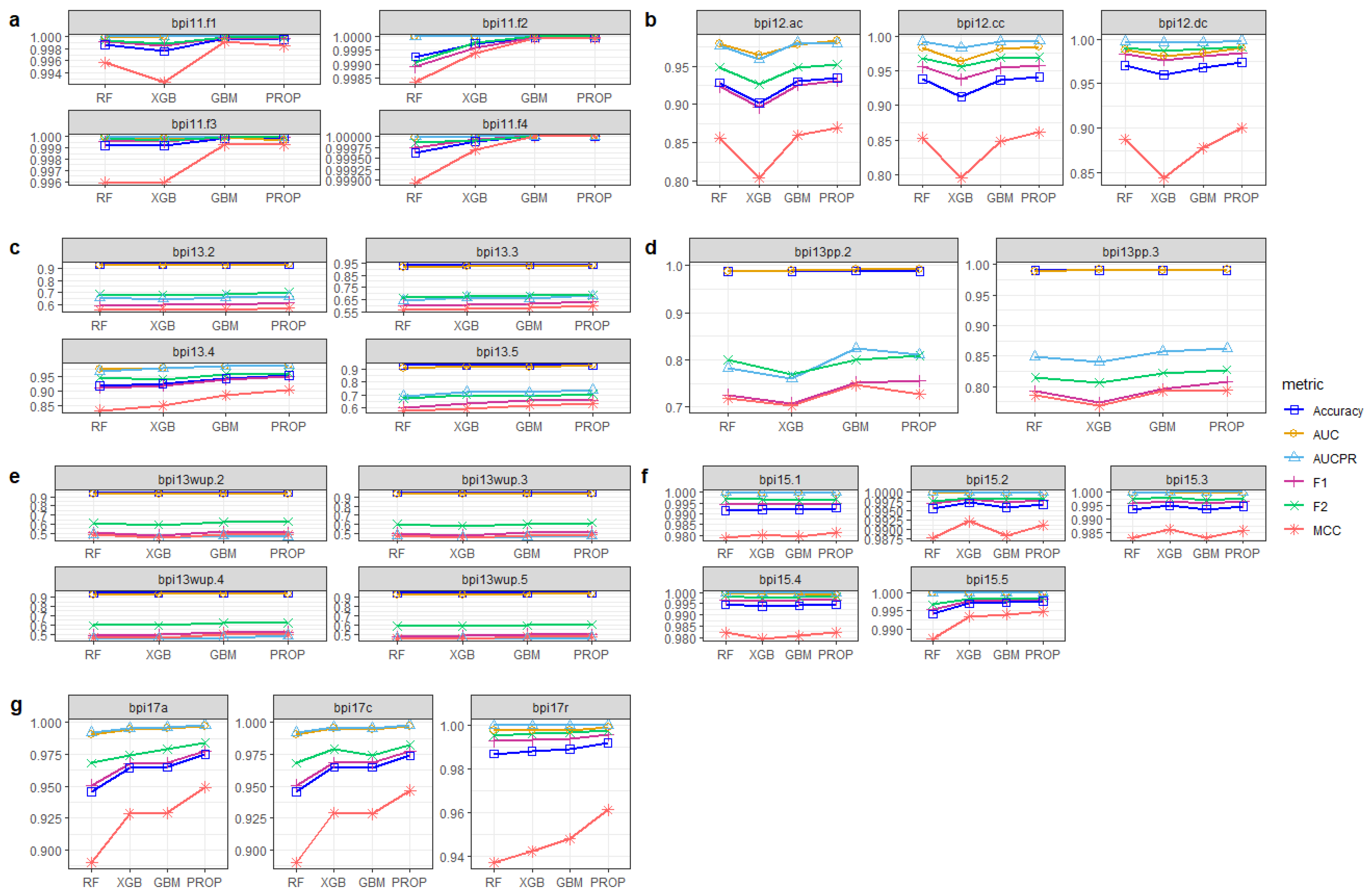
Figure 1 shows the average performance of the proposed and base models over different event logs. The proposed model (e.g., PROP) demonstrates its superiority over its base models, irrespective of the performance metrics considered. The performance increase obtained by the proposed model is more evident when the MCC metric is considered. Note that the MCC metric is an appropriate performance metric when the classes to be predicted are imbalanced, which is the case with most event logs considered in this paper (see Section 4.2). The relative performance increase in PROP with respect to the base models for each dataset and performance metric is reported numerically in

Table 2. Percentage improvement that the proposed model offers over base classifiers.

Dataset	Event Logs	Classifier $\mathcal{M}$	Classifier $\mathcal{N}$	F1	F2	MCC	Accuracy	AUCPR	AUC
BPIC11	bpi11.f1	PROP	RF	0.056	0.041	0.275	0.089	0.002	0.005
			XGB	0.121	0.099	0.597	0.193	0.001	0.002
			GBM	−0.014	−0.007	−0.069	−0.022	−0.001	−0.005
	bpi11.f2	PROP	RF	0.105	0.094	0.158	0.070	0.001	0.000
			XGB	0.035	0.020	0.053	0.023	0.000	0.000
			GBM	0.000	0.000	0.000	0.000	0.000	0.000
	bpi11.f3	PROP	RF	0.036	0.014	0.335	0.064	−0.008	−0.030
			XGB	0.036	0.027	0.335	0.064	−0.006	−0.019
			GBM	0.000	0.000	0.000	0.000	−0.008	−0.032
	bpi11.f4	PROP	RF	0.025	0.014	0.105	0.038	0.000	0.000
			XGB	0.007	0.008	0.030	0.011	0.000	0.000
			GBM	0.000	0.000	0.000	0.000	0.000	0.000
BPIC12	bpi12.ac	PROP	RF	0.813	0.398	1.570	0.697	0.361	0.308
			XGB	3.890	2.822	8.186	3.620	2.158	1.903
			GBM	0.575	0.399	1.149	0.505	−0.180	0.511
	bpi12.cc	PROP	RF	0.246	0.244	0.911	0.320	0.096	0.217
			XGB	2.176	1.509	8.233	3.084	1.041	2.161
			GBM	0.351	0.171	2.551	0.602	0.162	0.624
	bpi12.dc	PROP	RF	0.196	0.133	1.431	0.337	0.065	0.270
			XGB	0.861	0.478	6.651	1.499	0.192	0.947
			GBM	0.351	0.171	2.551	0.602	0.162	0.624
BPIC13	bpi13.2	PROP	RF	4.077	2.726	3.315	0.209	2.341	0.922
			XGB	3.465	3.379	0.722	0.177	3.804	0.752
			GBM	3.915	2.227	2.525	0.274	1.330	1.144
	bpi13.3	PROP	RF	5.452	3.014	6.289	0.691	5.522	1.365
			XGB	3.874	0.586	4.663	0.199	1.754	0.487
			GBM	0.287	2.366	1.551	0.016	1.074	0.232
	bpi13.4	PROP	RF	6.653	4.868	7.473	0.040	5.144	0.968
			XGB	6.157	4.549	7.712	0.024	6.809	0.746
			GBM	0.475	−0.326	−0.885	0.008	3.454	0.221
	bpi13.5	PROP	RF	4.707	2.702	3.450	−0.105	1.555	0.679
			XGB	3.168	3.513	4.121	−0.065	1.379	0.248
			GBM	−0.324	1.980	−1.052	0.016	2.424	0.226
	bpi13wup.2	PROP	RF	−0.494	2.428	1.012	−0.185	−4.976	0.517
			XGB	6.165	6.141	8.639	0.089	3.712	0.844
			GBM	−1.506	1.368	−0.431	−0.024	−2.088	0.094
	bpi13wup.3	PROP	RF	1.943	2.728	3.542	−0.201	−1.004	0.653
			XGB	6.612	5.765	8.989	0.024	5.328	0.834
			GBM	0.287	2.366	1.551	0.016	1.074	0.232
	bpi13wup.4	PROP	RF	6.653	4.868	7.473	0.040	5.144	0.968
			XGB	6.157	4.549	7.712	0.024	6.809	0.746
			GBM	0.475	−0.326	−0.885	0.008	3.454	0.221
	bpi13wup.5	PROP	RF	4.707	2.702	3.450	−0.105	1.555	0.679
			XGB	3.168	3.513	4.121	−0.065	1.379	0.248
			GBM	−0.324	1.980	−1.052	0.016	2.424	0.226
	bpi13pp.2	PROP	RF	4.136	1.087	1.315	0.075	3.654	0.498
			XGB	6.713	5.204	3.569	0.108	6.804	0.249
			GBM	0.459	1.010	−2.629	−0.058	−1.459	0.043
	bpi13pp.3	PROP	RF	1.850	1.544	1.012	−0.033	1.740	0.469
			XGB	4.380	2.657	3.299	0.025	2.689	0.128
			GBM	1.447	0.650	0.067	−0.058	0.697	0.320
BPIC15	bpi15.1	PROP	RF	0.073	−0.005	0.271	0.107	0.003	0.007
			XGB	0.039	0.009	0.119	0.053	0.007	0.015
			GBM	0.050	0.058	0.179	0.071	0.004	0.011
	bpi15.2	PROP	RF	0.080	0.061	0.351	0.123	−0.001	−0.003
			XGB	−0.024	−0.006	−0.102	−0.037	0.000	−0.001
			GBM	0.064	0.010	0.280	0.099	0.001	0.002
	bpi15.3	PROP	RF	0.070	0.041	0.285	0.105	0.002	0.006
			XGB	−0.011	−0.039	−0.051	−0.017	−0.001	−0.002
			GBM	0.069	0.071	0.286	0.105	0.001	0.004
	bpi15.4	PROP	RF	−0.001	−0.031	0.009	0.000	−0.021	−0.026
			XGB	0.052	0.083	0.281	0.085	−0.020	−0.024
			GBM	0.025	0.041	0.152	0.042	−0.017	−0.014
	bpi15.5	PROP	RF	0.275	0.179	0.762	0.350	0.005	0.009
			XGB	0.051	0.014	0.139	0.064	0.001	0.001
			GBM	0.029	0.032	0.080	0.037	0.003	0.004
BPIC17	bpi17a	PROP	RF	2.808	1.631	6.608	3.097	0.540	0.679
			XGB	0.967	0.989	2.244	1.069	0.206	0.262
			GBM	0.923	0.481	2.176	1.034	0.159	0.192
	bpi17c	PROP	RF	2.769	1.486	6.327	2.986	0.536	0.639
			XGB	0.928	0.846	1.975	0.960	0.201	0.223
			GBM	0.884	0.338	1.906	0.926	0.155	0.153
	bpi17r	PROP	RF	0.288	0.205	2.561	0.510	0.016	0.117
			XGB	0.227	0.143	2.011	0.403	0.015	0.112
			GBM	0.158	0.081	1.404	0.281	0.015	0.106

.

Among the base models, GBM emerges as the best-performing one. Teinemaa et al. [7], in their benchmark of outcome-based predictive model, reported XGB to be the superior classifier in this type of predictive problem. However, in their study, they did not consider GBM as a classifier, nor some of the performance metrics considered here, such as MCC and AUCPR. Our results show that the base model GBM generally outperforms XGB.

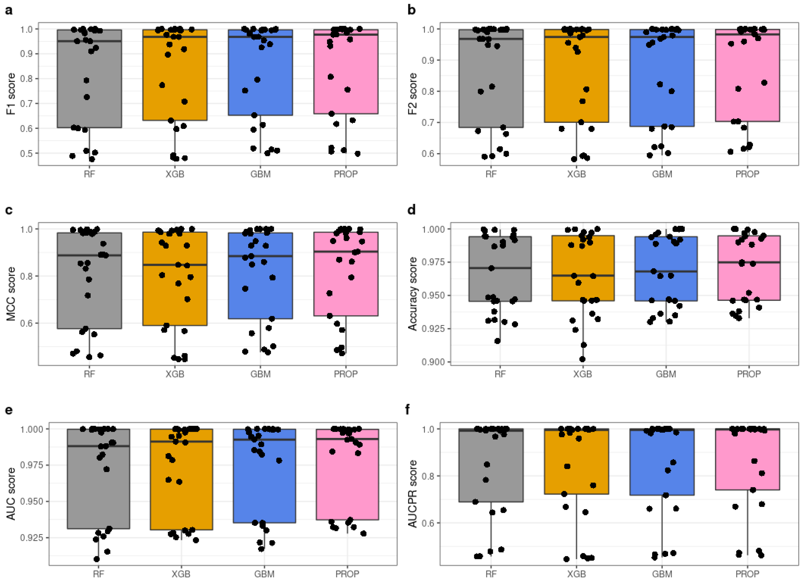
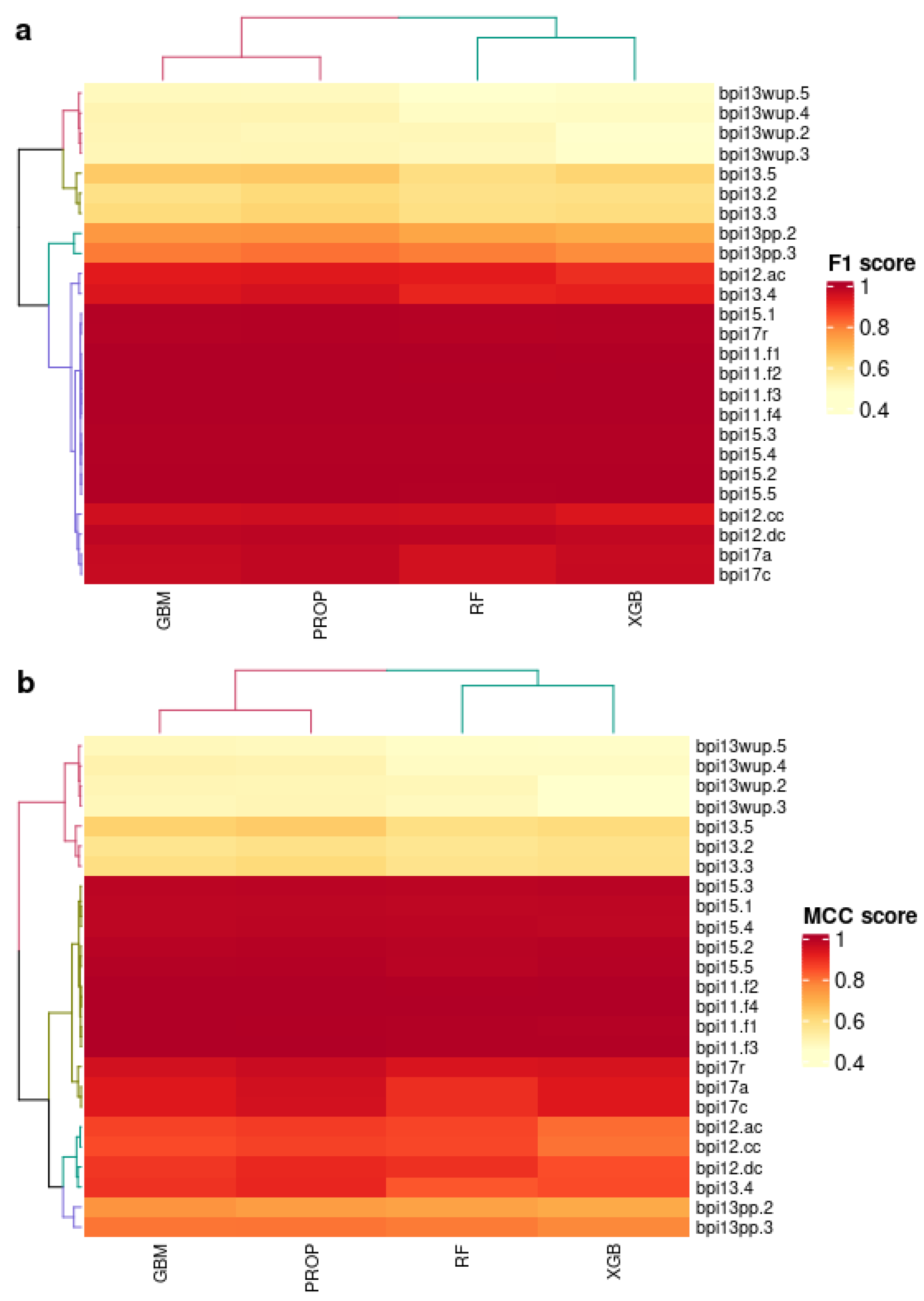
To better understand the superior performance of the proposed method, Figure 2 shows boxplots of the performance results achieved on all event logs. We can see that PROP is the best-performing model considering the median and the interquartile range on all the datasets considered in the experimental evaluation. Figure 3 shows the correlation plots for the F1-score and MCC performance metrics between the predictive models and all the datasets considered in the evaluation clustered using the performance achieved as a clustering measure. The performance achieved is indicated using a heatmap (the warmer the heatmap, the higher the performance achieved). We can see that the warmer colors are associated with the PROP model. More in detail, while all the classifiers achieve high performance on the BPI11 and BPI15 datasets, PROP shows better performance also on the other datasets, e.g., BPI17 and BPI12, where the performance achieved by the baseline models is normally lower.

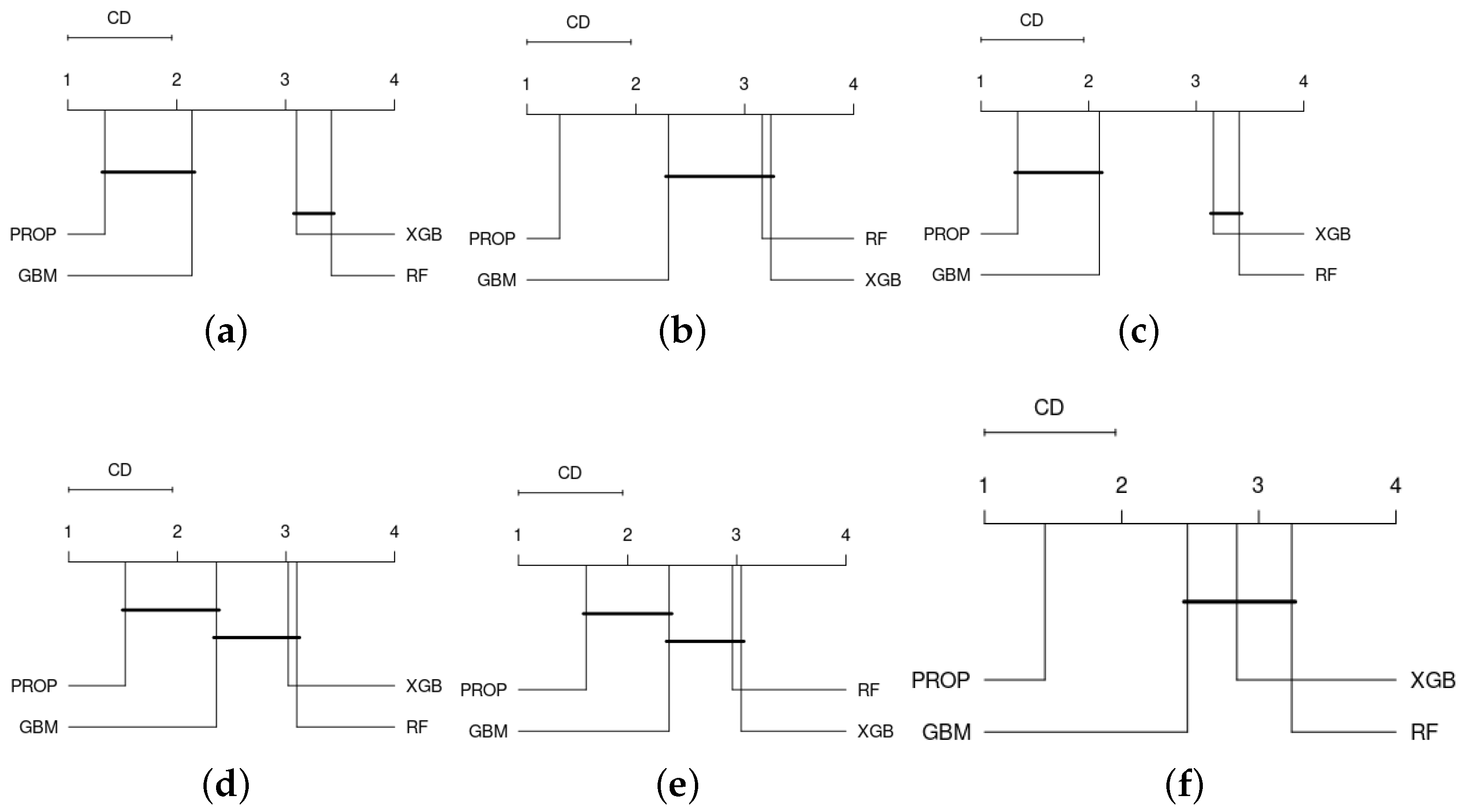
Finally, to assess whether the performance differences among the models considered in this evaluation are significant, Figure 4 shows the results of the Nemenyi test for different performance metrics. For each performance metric, the plot first ranks the models from best (on the left-hand side) to worst (on the right-hand side). Then, the models are grouped together if their average ranking falls below the critical distance CD—that is, the minimum distance in the test results indicating that the ranking differences are significant at the chosen level $\alpha$ of significance. While for the performance metrics F1-score, accuracy, and AUC the proposed model PROP is grouped with at least GBM—i.e., the ranking difference among the models, at least GBM, is not statistically significant—the model PROP remains alone and top-ranked for the performance metrics MCC and AUCPR. This indicates that, when considering MCC and AUCPR, not only is the performance achieved by PROP the highest among competing models, but also the performance difference is significant across the datasets considered.

In summary, the proposed method generally outperforms its base models. The performance increase of the proposed model appears to be higher for those datasets where predictive models normally achieve on average a lower performance. The performance increase achieved by the proposed model, particularly with respect to GBM, which emerges as the best-performing base model, is statistically significant when considering performance metrics more appropriate to evaluate the performance on imbalanced classification problems, e.g., MCC and AUCPR.

5. Conclusions

We have presented a stacked ensemble model using strong learners for addressing the problem of outcome-based predictive monitoring. The objective of the paper is to demonstrate that the proposed model outperforms the strong learners XGB, RF, and GBM that we have considered as base learners. The experimental evaluation, conducted on several publicly available event logs, demonstrated that this is the case: the proposed stacked ensemble generally outperforms the strong learners and this effect is more evident when performance metrics more suitable for classification using imbalanced datasets, such as AUCPR and MCC, are considered.

The research presented in this paper has several limitations. First, in the experimental evaluation, we considered only one specific combination of prefix encoding and bucketing. While this has been done to maintain the number of experiments manageable, we cannot assume that the results obtained considering different settings would suggest different conclusions. However, Teinemaa et al. [7] demonstrated in their extensive benchmark that the effect on the performance of different encoding and bucketing methods is lower in magnitude when compared to the choice of classifier. Second, in this work, we did not analyze the results obtained by prefix length. Our objective was to conduct a large number of experiments and to aggregate the results obtained in order to establish, with the support of statistical tests, whether the proposed stacking ensemble had a better overall performance than the baselines. To do so, we had to rely on standard performance measures on aggregated observations; so, we did not consider other measures of performance in outcome-based predictive monitoring, such as earliness or stability of the predictions.

The work presented here can be extended in several ways. First, event log datasets are typically imbalanced. Due to the fact that this might alter the effectiveness of the classification algorithm, it would be interesting to employ undersampling or oversampling approaches in order to better understand the pattern behavior of classification algorithms in those two distinct circumstances. Second, there has been significant progress in applying deep learning models for tabular data, with research often claiming that the models outperform the ensemble model—i.e., XGB—in some cases [30,31]. Additional research is very certainly necessary in this regard, especially to determine if deep learning models perform statistically better on tabular event log data.

References

- Van der Aalst, W.M. Process Mining: Data Science in Action; Springer: Berlin/Heidelberg, Germany, 2016. [Google Scholar]
- Márquez-Chamorro, A.E.; Resinas, M.; Ruiz-Cortés, A. Predictive monitoring of business processes: A survey. IEEE Trans. Serv. Comput. 2017, 11, 962–977. [Google Scholar] [CrossRef]
- Verenich, I.; Dumas, M.; Rosa, M.L.; Maggi, F.M.; Teinemaa, I. Survey and cross-benchmark comparison of remaining time prediction methods in business process monitoring. ACM Trans. Intell. Syst. Technol. 2019, 10, 1–34. [Google Scholar] [CrossRef]
- Evermann, J.; Rehse, J.R.; Fettke, P. Predicting process behaviour using deep learning. Decis. Support Syst. 2017, 100, 129–140. [Google Scholar] [CrossRef]
- Tama, B.A.; Comuzzi, M. An empirical comparison of classification techniques for next event prediction using business process event logs. Exp. Syst. Appl. 2019, 129, 233–245. [Google Scholar] [CrossRef]
- Tama, B.A.; Comuzzi, M.; Ko, J. An Empirical Investigation of Different Classifiers, Encoding, and Ensemble Schemes for Next Event Prediction Using Business Process Event Logs. ACM Trans. Intell. Syst. Technol. 2020, 11, 1–34. [Google Scholar] [CrossRef]
- Teinemaa, I.; Dumas, M.; Rosa, M.L.; Maggi, F.M. Outcome-oriented predictive process monitoring: Review and benchmark. ACM Trans. Knowl. Discov. Data 2019, 13, 17. [Google Scholar] [CrossRef]
- Senderovich, A.; Di Francescomarino, C.; Maggi, F.M. From knowledge-driven to data-driven inter-case feature encoding in predictive process monitoring. Inf. Syst. 2019, 84, 255–264. [Google Scholar] [CrossRef]
- Kim, J.; Comuzzi, M.; Dumas, M.; Maggi, F.M.; Teinemaa, I. Encoding resource experience for predictive process monitoring. Decis. Support Syst. 2022, 153, 113669. [Google Scholar] [CrossRef]
- Van der Laan, M.J.; Polley, E.C.; Hubbard, A.E. Super learner. Stat. Appl. Genet. Mol. Biol. 2007, 6. [Google Scholar] [CrossRef] [PubMed]
- Di Francescomarino, C.; Ghidini, C.; Maggi, F.M.; Milani, F. Predictive Process Monitoring Methods: Which One Suits Me Best? In Proceedings of the International Conference on Business Process Management, Sydney, Australia, 9–14 September 2018; Springer: Cham, Switzerland, 2018; pp. 462–479. [Google Scholar]
- Santoso, A. Specification-driven multi-perspective predictive business process monitoring. In Enterprise, Business-Process and Information Systems Modeling; Springer: Cham, Switzerland, 2018; pp. 97–113. [Google Scholar]
- Verenich, I.; Dumas, M.; La Rosa, M.; Nguyen, H. Predicting process performance: A white-box approach based on process models. J. Softw. Evol. Process 2019, 31, e2170. [Google Scholar] [CrossRef]
- Galanti, R.; Coma-Puig, B.; de Leoni, M.; Carmona, J.; Navarin, N. Explainable predictive process monitoring. In Proceedings of the 2020 2nd International Conference on Process Mining (ICPM), Padua, Italy, 5–8 October 2020; pp. 1–8. [Google Scholar]
- Rama-Maneiro, E.; Vidal, J.C.; Lama, M. Deep learning for predictive business process monitoring: Review and benchmark. arXiv 2020, arXiv:2009.13251. [Google Scholar] [CrossRef]
- Neu, D.A.; Lahann, J.; Fettke, P. A systematic literature review on state-of-the-art deep learning methods for process prediction. Artif. Intell. Rev. 2021, 55, 801–827. [Google Scholar] [CrossRef]
- Kratsch, W.; Manderscheid, J.; Röglinger, M.; Seyfried, J. Machine learning in business process monitoring: A comparison of deep learning and classical approaches used for outcome prediction. Bus. Inf. Syst. Eng. 2020, 63, 261–276. [Google Scholar] [CrossRef]
- Metzger, A.; Neubauer, A.; Bohn, P.; Pohl, K. Proactive Process Adaptation Using Deep Learning Ensembles. In Proceedings of the International Conference on Advanced Information Systems Engineering, Rome, Italy, 3–7 June 2019; Springer: Berlin/Heidelberg, Germany, 2019; pp. 547–562. [Google Scholar]
- Wang, J.; Yu, D.; Liu, C.; Sun, X. Outcome-oriented predictive process monitoring with attention-based bidirectional LSTM neural networks. In Proceedings of the 2019 IEEE International Conference on Web Services (ICWS), Milan, Italy, 8–13 June 2019; pp. 360–367. [Google Scholar]
- Folino, F.; Folino, G.; Guarascio, M.; Pontieri, L. Learning effective neural nets for outcome prediction from partially labelled log data. In Proceedings of the 2019 IEEE 31st International Conference on Tools with Artificial Intelligence (ICTAI), Portland, OR, USA, 4–6 November 2019; pp. 1396–1400. [Google Scholar]
- Pasquadibisceglie, V.; Appice, A.; Castellano, G.; Malerba, D.; Modugno, G. ORANGE: Outcome-oriented predictive process monitoring based on image encoding and cnns. IEEE Access 2020, 8, 184073–184086. [Google Scholar] [CrossRef]
- Wolpert, D.H. Stacked generalization. Neural Netw. 1992, 5, 241–259. [Google Scholar] [CrossRef]
- Bergstra, J.; Bengio, Y. Random search for hyper-parameter optimization. J. Mach. Learn. Res. 2012, 13, 281–305. [Google Scholar]
- Breiman, L. Random forests. Mach. Learn. 2001, 45, 5–32. [Google Scholar] [CrossRef]
- Friedman, J.H. Greedy function approximation: A gradient boosting machine. Ann. Stat. 2001, 29, 1189–1232. [Google Scholar] [CrossRef]
- Chen, T.; Guestrin, C. Xgboost: A scalable tree boosting system. In Proceedings of the 22nd ACM SIGKDD International Conference on Knowledge Discovery and Data Mining, San Francisco, CA, USA, 13–17 August 2016; pp. 785–794. [Google Scholar]
- Di Francescomarino, C.; Dumas, M.; Maggi, F.M.; Teinemaa, I. Clustering-based predictive process monitoring. IEEE Trans. Serv. Comput. 2016, 12, 896–909. [Google Scholar] [CrossRef]
- Saito, T.; Rehmsmeier, M. The precision-recall plot is more informative than the ROC plot when evaluating binary classifiers on imbalanced datasets. PLoS ONE 2015, 10, e0118432. [Google Scholar] [CrossRef] [PubMed]
- Chicco, D.; Jurman, G. The advantages of the Matthews correlation coefficient (MCC) over F1 score and accuracy in binary classification evaluation. BMC Genom. 2020, 21, 6. [Google Scholar] [CrossRef]
- Shwartz-Ziv, R.; Armon, A. Tabular data: Deep learning is not all you need. Inf. Fusion 2022, 81, 84–90. [Google Scholar] [CrossRef]
- Borisov, V.; Leemann, T.; Seßler, K.; Haug, J.; Pawelczyk, M.; Kasneci, G. Deep neural networks and tabular data: A survey. arXiv 2021, arXiv:2110.01889. [Google Scholar]
Figure 1.
(a–g) Performance comparison between the proposed ensemble (e.g., PROP) and its base learners across different datasets in terms of mean accuracy, AUC, AUCPR, F1, F2, and MCC scores.
Figure 2.
(a–f) Boxplots (center, median; box, interquartile range (IQR); whiskers, 1.5 × IQR) illustrating the average performance distribution of classification algorithms.
Figure 3.
(a,b) Correlation plot denoting clustered solution spaces. The color represents the performance score (e.g., low, yellow; high, red) of classifier, ranging from 0.4 to 1. For each performance metric, the datasets are roughly grouped based on the classification algorithms.
Figure 4.
Critical difference plot using Nemenyi Test (significant level, ) across performance metrics: F1 score (a), F2 score (b), Matthew correlation coefficient (MCC) score (c), accuracy score (d), area under ROC curve (AUC) score (e), and area under precision–recall curve (AUCPR) score (f).