Versatile Field-Programmable Analog Array Realizations of Power-Law Filters

Abstract

A structure suitable for implementing power-law low-pass and high-pass filter transfer functions is presented in this work. Through the utilization of a field-programmable analog array device, full programmability of the characteristics of the intermediate stages, as is required for realizing the rational integer-order transfer function that approximates the corresponding power-law function, was achieved, making the structure versatile. In addition, a comparison between power-law and fractional-order filters regarding the effect of the non-integer order was performed. The presented design examples are fully supported by experimental results.

1. Introduction

Integer-order analog signal processing requires the employment of fundamental filtering operations, such as the low-pass (LP) and high-pass (HP) filter functions described, respectively, by:

$$H_{LP}\left(s\right)=\frac{{\omega }_0}{s+{\omega }_0},$$

(1a)

$$H_{HP}\left(s\right)=\frac{s}{s+{\omega }_0}.$$

(1b)

The characteristic frequency ${\omega }_0$ is the pole frequency of the transfer function and determines the half-power frequency $\left({\omega }_h\right)$, where a $-3\mathrm{dB}$ deviation of the maximum value of the gain is observed.

Non-integer order signal processing has received significant research interest in the following fields [1,2,3,4,5,6]. The first field is electrical engineering, for implementing filters and oscillators [5,7,8,9,10,11,12,13,14,15], chaotic systems [16], sensor systems [17], and control systems [2,18,19,20,21]. This originates from the fact that both filters and oscillators offer additional degrees of freedom due to the non-integer order, which opens the door for scaling the characteristic frequencies of the filters/oscillators, as well as for precisely controlling the gradient of the transition from the pass-band to the stop-band. The first fact is very important in biomedical applications, where large time constants are required, while the second is a very attractive feature in acoustic applications (e.g., shelving filters) for implementing equalizers with fine tuning [22], as well as in control applications (e.g., mechatronic systems), where loop-shaping tuning is performed to achieve the required frequency domain specifications, such as gain, margin etc. [23]. The second field is biology/bio-medicine and chemistry, including electrochemical impedance spectroscopy (EIS), for the description of the behavior of biological tissues, and electrical models of human organs/systems [24,25,26,27,28]. The third field is renewable energy systems, for the modeling of super-capacitors, batteries, and fuel cells [29]. It has been proven that when employing non-integer order transfer functions, the behavior/characteristics of the aforementioned systems are represented in a more realistic way compared with their representation with integer-order counterparts.

Non-integer order transfer functions can be derived through:

(a) the employment of non-integer Laplace operators. Considering (1a) and (1b), this can be done through the substitution operation $s\to s^{\alpha }$, with $0<\alpha <1$ being the order of the operator. The resulting filters are denoted in the literature as fractional-order filters [7,8,15].

(b) the employment of transfer functions, which are derived from their integer-order counterparts, raised to a non-integer exponent. Following this, the corresponding transfer functions, which are derived from (1a) and (1b), will have the form of $H_{LP}^{\beta }$ and $H_{HP}^{\beta }$ respectively, with $0<\beta <1$ denoting the associated order. These types of filters are referred to as power-law filters in the literature [22,30].

Fractional-order filters cannot be implemented directly because fractional-order elements are not currently available. Their realization can be based on emulators that approximate the elements’ behavior and substitute the corresponding integer-order elements, or based on an integer-order rational transfer function, which approximates the original fractional-order function. The situation in power-law filters is different, in the sense that fractional-order elements are not required and, consequently, their implementation is always performed on a transfer-function basis using appropriate approximation techniques. Power-law filters were initially introduced and studied in [30], where an op-amp-based implementation was presented. In [22], voltage current conveyors (VCII) were utilized as active elements for implementing power-law filters for acoustic applications. In [12], an optimization of power-law filter functions was performed, and the presented implementation was performed using Current-Feedback Operational Amplifiers (CFOAs) as active elements The aforementioned configurations are simple solutions, perfectly working for cases of filters with pre-defined type and frequency characteristics, as no programmability or tuning of the resistors’ and/or capacitors’ values is provided.

The contribution made in this work is the utilization of a field-programmable analog array (FPAA)-based power-law filter configuration, which offers tuning capability in power-law filters. According to the authors’ best knowledge, such a structure has not yet been presented in the literature.

The paper is organized as follows: a comparison between fractional-order (FO) and power-law (PL) filters is performed in Section 2 to demonstrate their main differences. A functional block diagram (FBD) realization of power-law filters is presented in Section 3, and its FPAA-based implementation, as well as the derived experimental results, are given in Section 4.

2. Comparison between Fractional-Order and Power-Law Filters

2.1. Fractional-Order Filters

The transfer function that describes a low-pass filter of order $0<\alpha <1$ is given by:

$$H_{FO-LP}\left(s\right)=\frac{{\omega }_0^{\alpha }}{s^{\alpha }+{\omega }_0^{\alpha }},$$

(2)

with the magnitude frequency response being described by the expression:

$$\mid H_{FO-LP}\left(\omega \right)\mid =\frac{1}{\sqrt{{\left(\frac{\omega }{{\omega }_0}\right)}^{2\alpha }+2{\left(\frac{\omega }{{\omega }_0}\right)}^{\alpha }cos\left(\frac{\alpha \pi }{2}\right)+1}}.$$

(3)

Although the pole frequency is still equal to ${\omega }_0$, the half-power frequency is different from the pole frequency [8], and is expressed as:

$${\omega }_{h,FO-LP}={\omega }_0{\left[\sqrt{1+{cos}^2\left(\frac{\alpha \pi }{2}\right)}-cos\left(\frac{\alpha \pi }{2}\right)\right]}^{1/\alpha }.$$

(4)

In the case of a fractional-order high-pass filter, the transfer function in (1b) becomes:

$$H_{FO-HP}\left(s\right)=\frac{s^{\alpha }}{s^{\alpha }+{\omega }_0^{\alpha }}.$$

(5)

The magnitude response of (5) is given by the expression:

$$\mid H_{FO-HP}\left(\omega \right)\mid =\frac{{\left(\frac{\omega }{{\omega }_0}\right)}^{\alpha }}{\sqrt{{\left(\frac{\omega }{{\omega }_0}\right)}^{2\alpha }+2{\left(\frac{\omega }{{\omega }_0}\right)}^{\alpha }cos\left(\frac{\alpha \pi }{2}\right)+1}},$$

(6)

and the half-power frequency by the expression:

$${\omega }_{h,FO-HP}={\omega }_0{\left[\sqrt{1+{cos}^2\left(\frac{\alpha \pi }{2}\right)}+cos\left(\frac{\alpha \pi }{2}\right)\right]}^{1/\alpha }.$$

(7)

2.2. Power-Law Filters

The transfer function of a power-law low-pass filter of order $0<\beta <1$ is given by:

$$H_{PL-LP}\left(s\right)={\left(\frac{{\omega }_0}{s+{\omega }_0}\right)}^{\beta },$$

(8)

and the expressions of the magnitude frequency response and the half-power frequency are given in (9) and (10), respectively.

$$\mid H_{PL-LP}\left(\omega \right)\mid =\frac{1}{{\left[{\left(\frac{\omega }{{\omega }_0}\right)}^2+1\right]}^{\beta /2}},$$

(9)

$${\omega }_{h,PL-LP}={\omega }_0·\sqrt{2^{1/\beta }-1}.$$

(10)

The corresponding expressions of a power-law high-pass filter are given by (11)–(13).

$$H_{PL-HP}\left(s\right)={\left(\frac{s}{s+{\omega }_0}\right)}^{\beta },$$

(11)

$$\mid H_{PL-HP}\left(\omega \right)\mid =\frac{{\left(\frac{\omega }{{\omega }_0}\right)}^{\beta }}{{\left[{\left(\frac{\omega }{{\omega }_0}\right)}^2+1\right]}^{\beta /2}},$$

(12)

$${\omega }_{h,PL-HP}=\frac{{\omega }_0}{\sqrt{2^{1/\beta }-1}}.$$

(13)

The slope of the stopband attenuation for the fractional-order and power-law filters is $\mp 20·\alpha \mathrm{dB}/\mathrm{dec}$ and $\mp 20·\beta \mathrm{dB}/\mathrm{dec}$, respectively, making both types equivalent in terms of the gradient of the magnitude response. According to (2), (5), (8), and (11), they also have the same pole frequency ${\omega }_0$. Considering (4), (7), (10), and (13), it is derived that the half-power frequencies of both types of low-pass and high-pass filters depends on the pole frequency, as well as on the order. The pole frequency determines the reference point, while the order determines the distances (equal in logarithmic scale) around the pole frequency; i.e., $\sqrt{{\omega }_{h,FO-LP}·{\omega }_{h,FO-HP}}=\sqrt{{\omega }_{h,PL-LP}·{\omega }_{h,PL-HP}}={\omega }_0$.

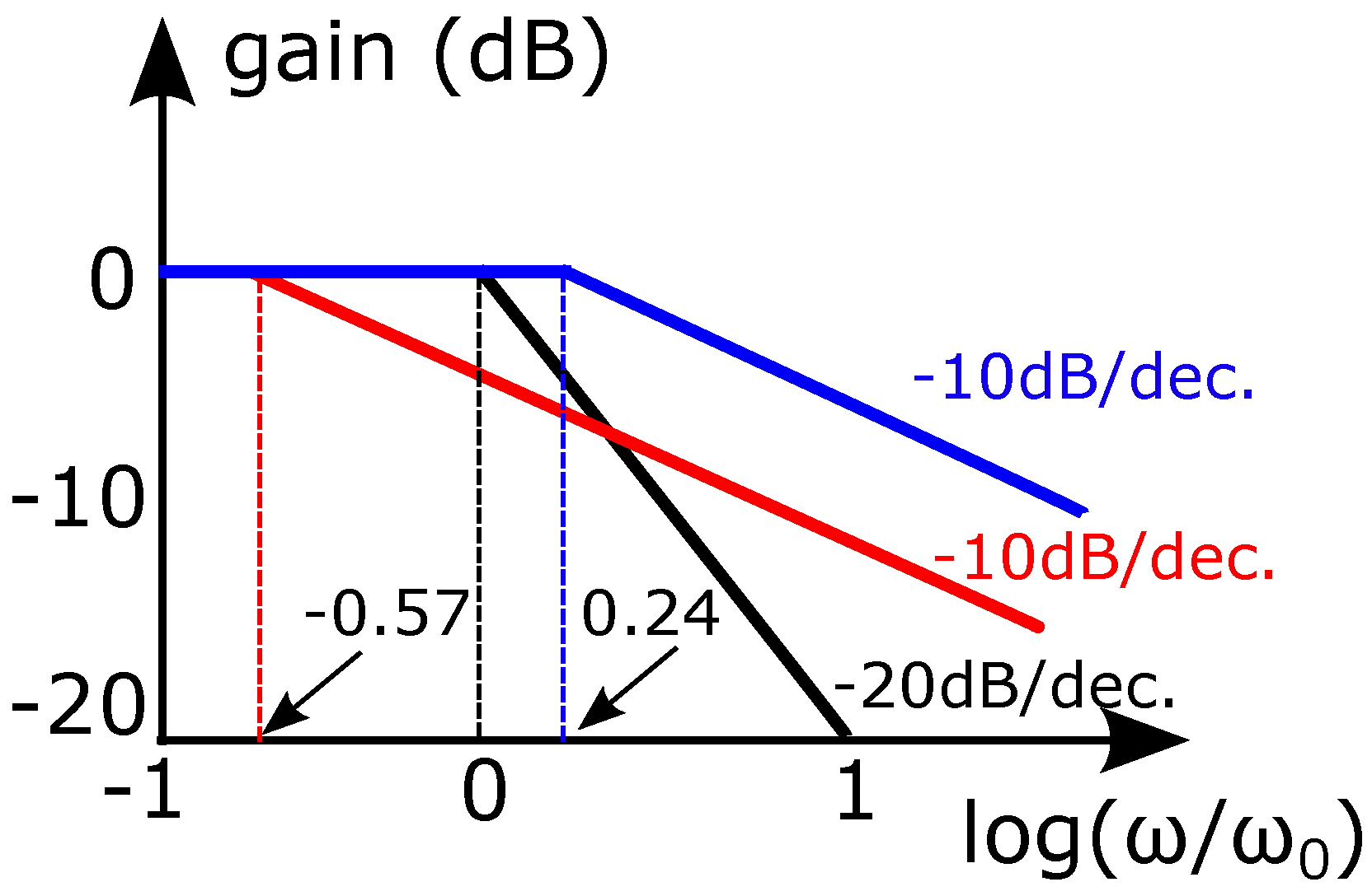
The main difference appertains to the relative location of the half-power frequencies with regards to the pole frequency. From the aforementioned expressions, the following conclusions are obtained: the location of the half-power frequencies of the low-pass filters is determined by the conditions ${\omega }_{h,FO-LP}<{\omega }_0$ and ${\omega }_{h,PL-LP}>{\omega }_0$, while for the high-pass filters, ${\omega }_{h,FO-HP}>{\omega }_0$ and ${\omega }_{h,PL-HP}<{\omega }_0$. Therefore, power-law filters are preferable in the case that the cutoff frequency of the low-pass filter must be greater than the pole frequency, or the cutoff frequency of the high-pass filter must be smaller than the pole frequency. In order to demonstrate the above findings, let us consider the case of low-pass filters with $\alpha =\beta =0.5$. The corresponding Bode plots are shown in Figure 1, where the effect of the type of the filter on the location of the realized half-power frequencies is evident.

It must be mentioned at this point that power-law filters are also capable of implementing locations of the half-power frequency opposite to the aforementioned ones, just by considering an order of $1<\beta <2$. This is realized by analyzing the transfer functions in (8) or (11) as products of a power-law term of order ($1-\beta$) and an integer-order term.

3. Realization of Power-Law Filters

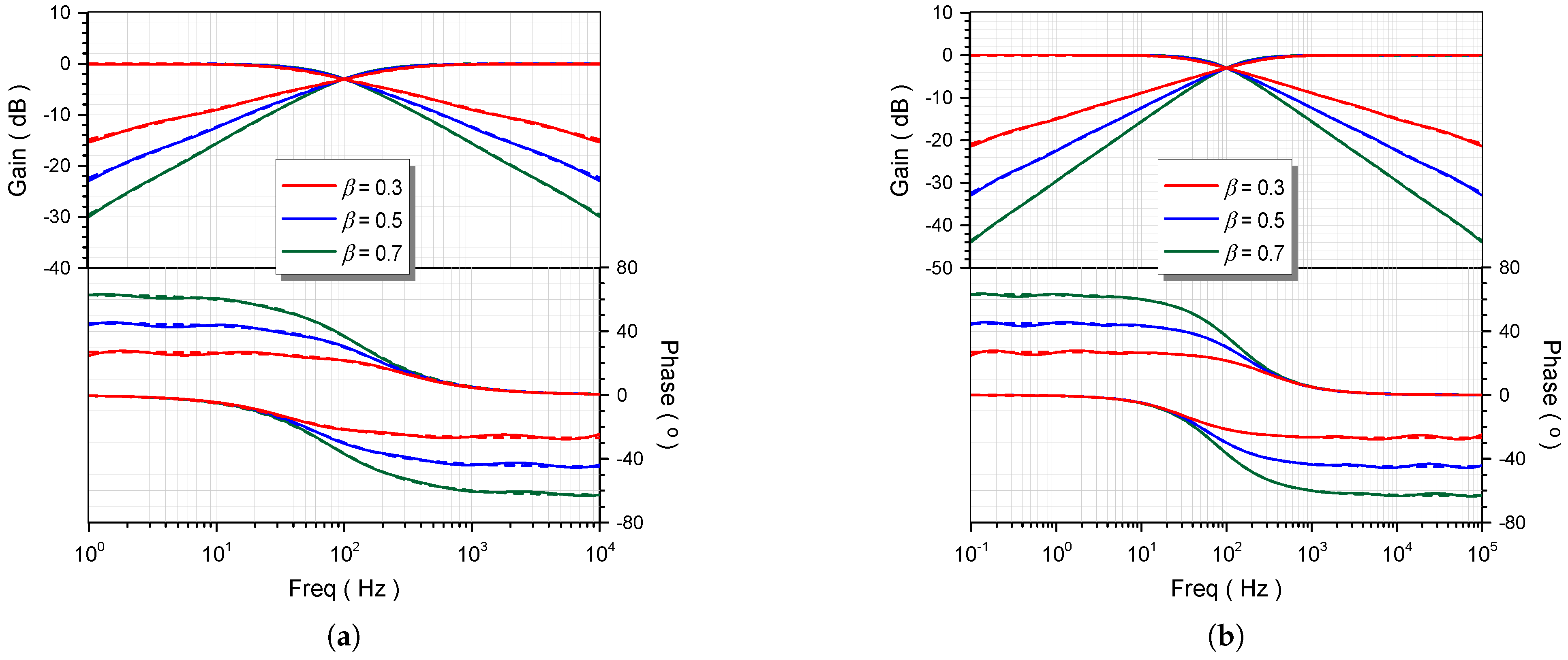
The approximation of the transfer functions in (8) and (11) can be performed through the utilization of the curve-fitting-based approximation technique [20,30]. Assuming third and fifth-order approximations, the derived MATLAB gain and phase frequency responses are in the ranges $\left[{10}^0,{10}^{+4}\right]\mathrm{Hz}$ and $\left[{10}^{-1},{10}^{+5}\right]\mathrm{Hz}$, respectively, are provided in the plots of Figure 2. As both cases offer the same level of accuracy, just for demonstration purposes, the third-order approximation in the range $\left[{10}^0,{10}^{+4}\right]\mathrm{Hz}$, will be considered. Therefore, the derived integer-order rational transfer function has the general form of:

$$H_{approx}\left(s\right)=\frac{A_3{s}^3+A_2{s}^2+A_{1}s+A_0}{s^3+B_2{s}^2+B_{1}s+B_0}.$$

(14)

Considering that the desired half-power frequency is $f_h=100\mathrm{Hz}$, the values of these factor, for approximating the behavior of low-pass and high-pass filters of various orders within the frequency range $\left[{10}^0,{10}^{+4}\right]\mathrm{Hz}$ are summarized in

Table 1. Coefficients of the transfer function in (14) for approximating LP and HP power-law filters [30].

Parameter	PL LP/HP Filter
	$\mathit{\beta }\mathbf{=}\mathbf{0.3}$	$\mathit{\beta }\mathbf{=}\mathbf{0.5}$	$\mathit{\beta }\mathbf{=}\mathbf{0.7}$
$A_0$	2.856 × 1010/2.738 × 105	4.396 × 1010/5.065 × 104	4.68 × 1010/1.145 × 104
$A_1$	4.953 × 107/4.925 × 104	4.26 × 107/1.618 × 104	3.025 × 107/7119
$A_2$	9128/676.8	4610/378.7	2155/253.1
$A_3$	0.1286/0.9885	0.03656/0.9899	0.008776/0.992
$B_0$	2.889 × 1010/2.13 × 106	4.441 × 1010/1.386 × 106	4.718 × 1010/1.304 × 106
$B_1$	8.696 × 107/1.672 × 105	1.003 × 108/1.087 × 105	9.634 × 107/9.641 × 104
$B_2$	3.099 × 104/1188	3.098 × 104/891.9	2.919 × 104/806.2

.

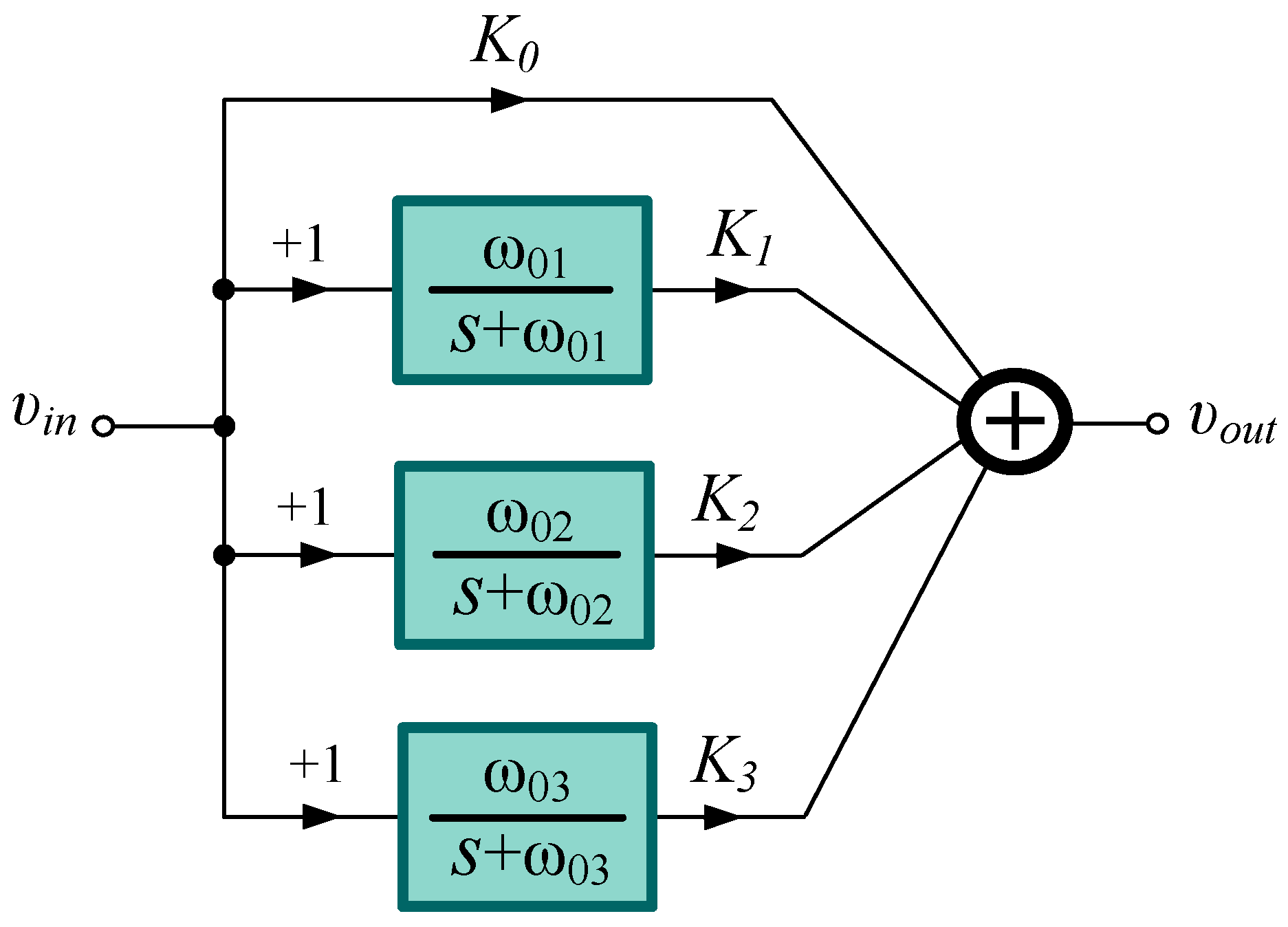
The implementation of (14) can be done by the following ways: (a) cascade connection of intermediate filter sections, (b) multi-feedback configuration of intermediate filter sections (series connection), and (c) sum of intermediate filter sections. Although the structure derived from the first technique is simpler than those derived from the other techniques, it suffers from increased sensitivity. On the other hand, the other two techniques suffer from increased circuit complexity and, consequently, power consumption. The implementation of the approximate function is performed following the method introduced in [31]. Applying the partial fraction expansion (PFE) technique to the function in (14), the obtained expression is a sum of integer-order low-pass terms and a constant factor, as described in:

$$H_{PFE}\left(s\right)=K_0+\frac{K_1·{\omega }_{01}}{s+{\omega }_{01}}+\frac{K_2·{\omega }_{02}}{s+{\omega }_{02}}+\frac{K_3·{\omega }_{03}}{s+{\omega }_{03}}.$$

(15)

In particular, considering that r and p are the residues and poles of (14), respectively, the parameters in (15) are calculated following the rules of thumb: $K_0=A_3$, $K_i=r_i/\left|p_i\right|$ and ${\omega }_{0i}=\left|p_i\right|$, $i=1,2,3$. The associated functional block diagram is formed as described in Figure 3.

The calculated values of scaling factors and time constants $\left({\tau }_i=\raisebox{1ex}{$1$}\!\left/ \!\raisebox{-1ex}{${\omega }_{0i}$}\right.\right)$ indicatively for LP and HP power-law filters of orders $\beta =\left\{0.3,0.5,0.7\right\}$ are summarized in

Table 2. Scaling factors and time constants for realizing the LP and HP power-law filters described by (14) for the coefficients of Table 1, using the PFE-based function in (15).

Parameter	PL LP/HP Filter
	$\mathit{\beta }\mathbf{=}\mathbf{0.3}$	$\mathit{\beta }\mathbf{=}\mathbf{0.5}$	$\mathit{\beta }\mathbf{=}\mathbf{0.7}$
$K_0$	0.129/0.988	0.0365/0.99	0.00878/0.99
$K_1$	0.153/−0.445	0.0886/−0.631	0.0374/−0.793
$K_2$	0.262/−0.262	0.233/−0.233	0.1525/−0.1525
$K_3$	0.445/−0.153	0.631/−0.0886	0.793/−0.0374
${\tau }_1$$\left(\mathrm{ms}\right)$	35.84/0.971	36.5/1.33	39.22/1.506
${\tau }_2$$\left(\mathrm{ms}\right)$	371.75/6.85	324.7/7.81	321.5/7.87
${\tau }_3$$\left(\mathrm{ms}\right)$	2.604/70.67	1.9/69.35	1.68/64.52

. The realization of filters of orders greater than 1 can be performed using an extra integer-order bilinear filter of the same type as the power-law filter.

4. Experimental Results

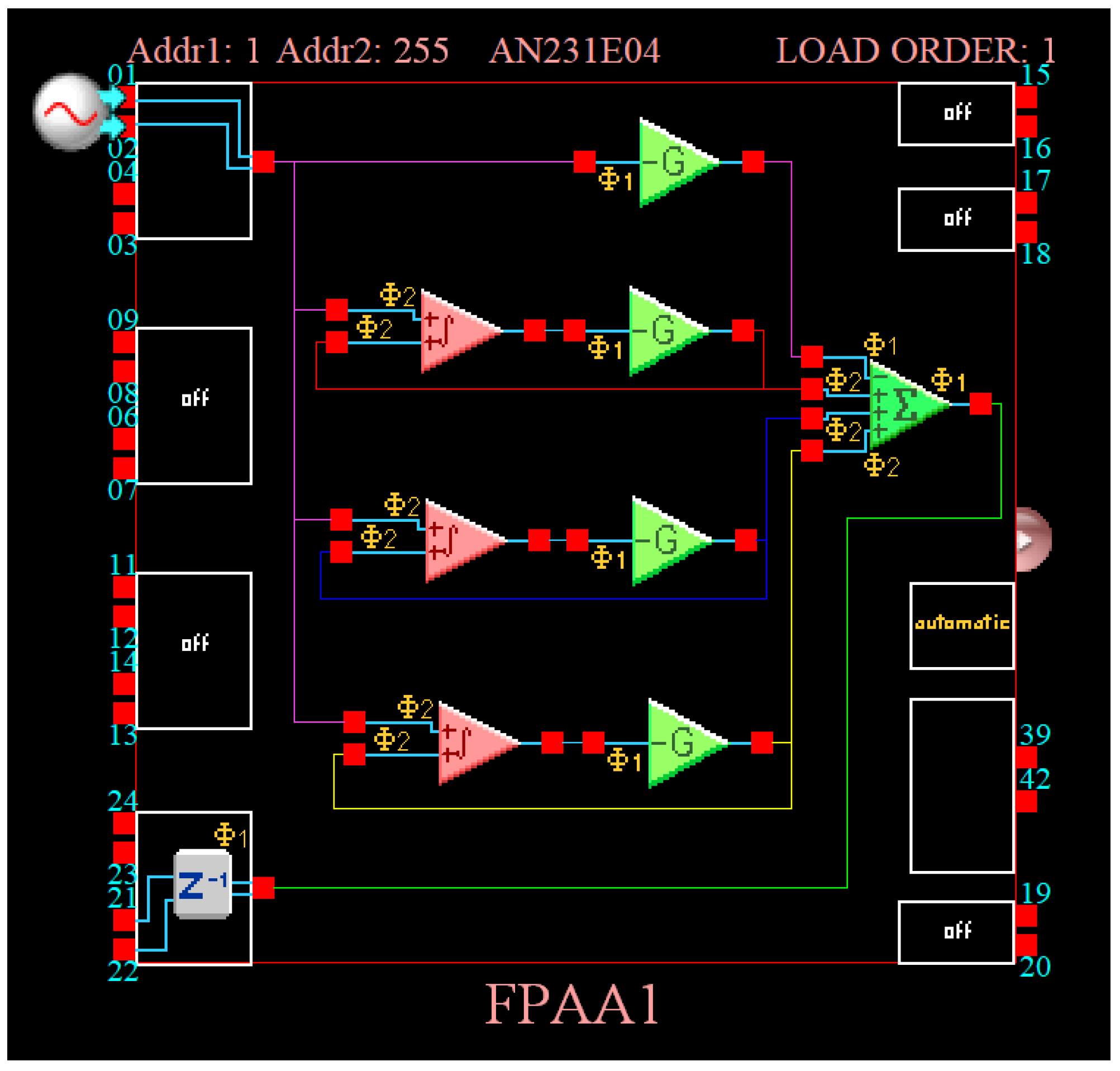
The experimental evaluation was performed using the Anadigm AN231K04 FPAA development board, programmed through the AnadigmDesigner^®2 EDA software [32]. The PFE-based configuration depicted in Figure 3 was used for realizing the design in Figure 4, where SumIntegrator, SumDiff, and GainHold configurable analogue modules (CAMs) were utilized, as described in

Table 3. Realized filter parameters of the CAMs of the design in Figure 4.

CAM	CAM Parameter	Realized Filter Parameter
GainHold	Gain	1
SumIntegrator1 + GainHold1	Integrator Constant × Gain	${\tau }_1$
SumIntegrator2 + GainHold2	Integrator Constant × Gain	${\tau }_2$
SumIntegrator3 + GainHold3	Integrator Constant × Gain	${\tau }_3$
SumDiff	Gain1	$K_0$
	Gain2	$K_1$
	Gain3	$K_2$
	Gain4	$K_3$

. There is a trade-off between the order of the approximation and the required hardware. As FPAA embeds four AN231E04 chips, each one having eight CAMs, it is obvious that when increasing the order, the number of required AN231E04 chips will be also increased. In the specific implementation, one chip is required. In the case that an approximation of greater order (e.g., 4 or 5) has been employed, then two or more chips would be required. The maximum frequency of the operation of the implemented filters depends on the chosen clock frequency, which is $f_{clk}$ = 100 kHz. Owing to the switched-capacitor nature of the stages included in the FPAA, the maximum operation frequency of the filters was $f_{max}=0.1·f_{clk}$ = 10 kHz.

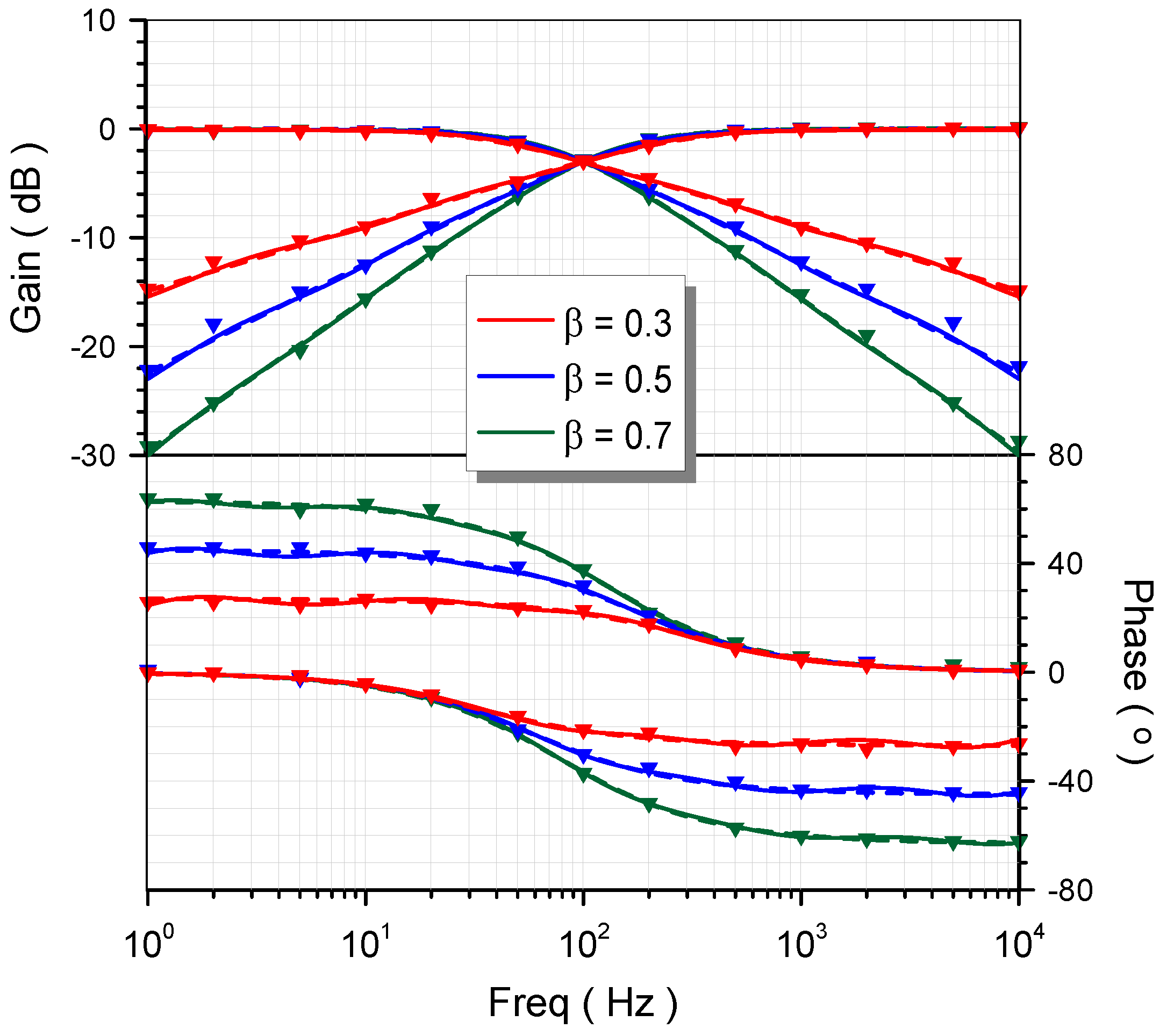
The experimental gain and phase frequency responses for the LP and HP filters of orders $\beta =\left\{0.3,0.5,0.7\right\}$ within the range $\left[{10}^0,{10}^{+4}\right]\mathrm{Hz}$ are given in Figure 5, indicated by triangle symbols, along with the respective results derived from the curve-fitting-based approximation (solid lines) and the theory (dashed lines). In addition, the experimental values of the critical characteristics for each case are presented in

Table 4. Frequency characteristics of LP filter responses in Figure 5.

Order	Parameter
	${\mathit{f}}_{\mathit{h}}\mathbf{\left(}\mathbf{Hz}\mathbf{\right)}$		Slope $\mathbf{\left(}\mathbf{dB/dec}\mathbf{\right)}$
	Experiment	Theory	Experiment	Theory
0.3	98.9	100	−5.9	−6
0.5	99.4	100	−9.65	−10
0.7	100	100	−13.5	−14

and

Table 5. Frequency characteristics of the HP filter responses in Figure 5.

Order	Parameter
	${\mathit{f}}_{\mathit{h}}\mathbf{\left(}\mathbf{Hz}\mathbf{\right)}$		Slope $\mathbf{\left(}\mathbf{dB/dec}\mathbf{\right)}$
	Experiment	Theory	Experiment	Theory
0.3	98.6	100	+5.7	+6
0.5	99	100	+9.7	+10
0.7	100	100	+13.6	+14

, with the respective theoretically calculated values given between parentheses.

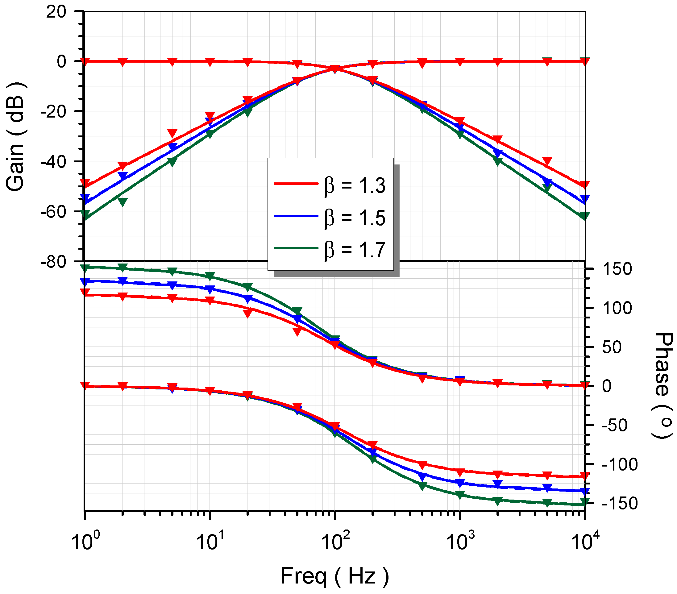
The corresponding results for orders $\beta =\left\{1.3,1.5,1.7\right\}$, which were obtained through the direct connection of the previously derived outputs with a first-order LP/HP filter, are given in Figure 6 and

Table 6. Frequency characteristics of LP filter responses in Figure 6.

Order	Parameter
	${\mathit{f}}_{\mathit{h}}\mathbf{\left(}\mathbf{Hz}\mathbf{\right)}$		Slope $\mathbf{\left(}\mathbf{dB/dec}\mathbf{\right)}$
	Experiment	Theory	Experiment	Theory
1.3	99.5	100	−25.6	−26
1.5	100	100	−28.85	−30
1.7	99.4	100	−32.8	−34

and

Table 7. Frequency characteristics of HP filter responses in Figure 6.

Order	Parameter
	${\mathit{f}}_{\mathit{h}}\mathbf{\left(}\mathbf{Hz}\mathbf{\right)}$		Slope $\mathbf{\left(}\mathbf{dB/dec}\mathbf{\right)}$
	Experiment	Theory	Experiment	Theory
1.3	99.2	100	+26.9	+26
1.5	98.8	100	+30.5	+30
1.7	98.6	100	+32	+34

.

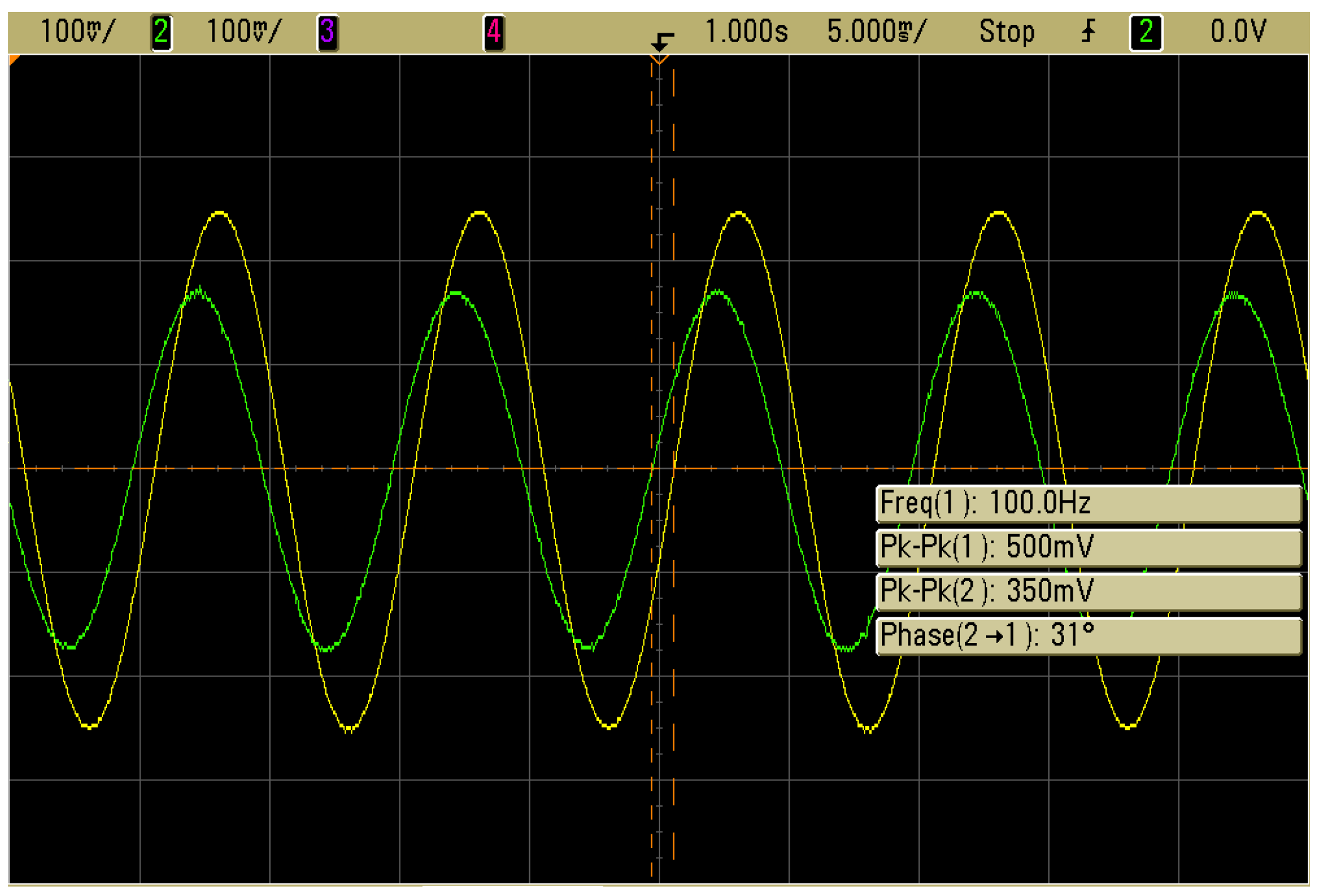
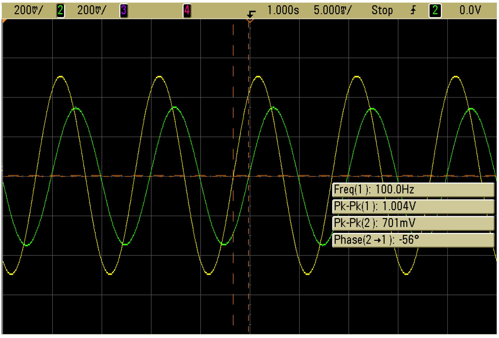
The efficient performance of the presented implementations in the time domain was also verified by simulating the filter with a sinusoidal signal of frequency $f=100\mathrm{Hz}$. Indicatively, the results in the case of an HP filter of order $\beta =0.5$ and an LP filter of order $\beta =1.5$ are presented, with the obtained waveforms being shown in Figure 7 and Figure 8. The measured values of the gain and phase are $-3.1\mathrm{dB}$ (theor. $-3\mathrm{dB}$) and $31°$ (theor. $30.45°$) for the HP filter, and $-3.09\mathrm{dB}$ (theor. $-3\mathrm{dB}$) and $-56°$ (theor. $-56.2°$) for the LP filter, respectively. Hence, the obtained results confirm the accurate performance of the presented topology.

5. Conclusions

By exploiting the advantage of the variety of signal processing operations that FPAAs offer, including integration/differentiation, summation/subtraction, scaling, filtering, and the fact that the intermediate blocks are interconnected through programmable buses [16,33], various types of power-law filters were implemented and experimentally verified. The price paid for the offered on-the-fly programmability is the restriction on the maximum frequency of operation, which originates from the switched-capacitor nature of the blocks of the FPAA. Other solutions could be conventional active-RC circuits, where the required discrete components are commercially available but the benefit of easy programmability of the time constants and scaling factors will be lost, or the utilization of active cells such as operational transconductance amplifiers (OTAs), where the programmability is performed through appropriate bias voltages/currents [34]. This solution offers a much higher maximum frequency of operations than that offered by the FPAAs, but it suffers from limited linearity due to the small-signal nature of the transconductance parameter used for realizing the time constants and scaling factors [9].

References

- Tsirimokou, G.; Psychalinos, C.; Elwakil, A. Design of CMOS Analog Integrated Fractional-Order Circuits: Applications in Medicine and Biology; Springer: Berlin/Heidelberg, Germany, 2017. [Google Scholar]
- Kochubei, A.; Luchko, Y.; Tarasov, V.E.; Petráš, I. Handbook of Fractional Calculus with Applications; De Gruyter: Berlin, Germany, 2019; Volume 1. [Google Scholar]
- Srivastava, H.M. Fractional-order integral and derivative operators and their applications. Mathematics 2020, 8, 1016. [Google Scholar] [CrossRef]
- Radwan, A.G.; Khanday, F.A.; Said, L.A. Fractional-Order Design: Devices, Circuits, and Systems; Elsevier: Amsterdam, The Netherlands, 2021. [Google Scholar]
- Muresan, C.I.; Birs, I.R.; Dulf, E.H.; Copot, D.; Miclea, L. A review of recent advances in fractional-order sensing and filtering techniques. Sensors 2021, 21, 5920. [Google Scholar] [CrossRef] [PubMed]
- Bertsias, P.; Kapoulea, S.; Psychalinos, C.; Elwakil, A.S. A collection of interdisciplinary applications of fractional-order circuits. In Fractional Order Systems; Elsevier: Amsterdam, The Netherlands, 2022; pp. 35–69. [Google Scholar]
- Radwan, A.G.; Soliman, A.M.; Elwakil, A.S. First-order filters generalized to the fractional domain. J. Circuits Syst. Comput. 2008, 17, 55–66. [Google Scholar] [CrossRef]
- Tsirimokou, G.; Psychalinos, C.; Elwakil, A.S. Fractional-order electronically controlled generalized filters. Int. J. Circuit Theory Appl. 2017, 45, 595–612. [Google Scholar] [CrossRef]
- Ahmed, O.I.; Yassin, H.M.; Said, L.A.; Psychalinos, C.; Radwan, A.G. Implementation and analysis of tunable fractional-order band-pass filter of order 2α. AEU-Int. J. Electron. Commun. 2020, 124, 153343. [Google Scholar] [CrossRef]
- Kubanek, D.; Koton, J.; Dvorak, J.; Herencsar, N.; Sotner, R. Optimized design of OTA-based gyrator realizing fractional-order inductance simulator: A comprehensive analysis. Appl. Sci. 2021, 11, 291. [Google Scholar] [CrossRef]
- Langhammer, L.; Sotner, R.; Dvorak, J.; Jerabek, J.; Andriukaitis, D. Reconnection–less Reconfigurable Fractional–Order Current–Mode Integrator Design with Simple Control. IEEE Access 2021, 9, 136395–136405. [Google Scholar] [CrossRef]
- Mahata, S.; Herencsar, N.; Kubanek, D. On the Design of Power Law Filters and Their Inverse Counterparts. Fractal Fract. 2021, 5, 197. [Google Scholar] [CrossRef]
- Mijat, N.; Jurisic, D.; Moschytz, G.S. Analog Modeling of Fractional-Order Elements: A Classical Circuit Theory Approach. IEEE Access 2021, 9, 110309–110331. [Google Scholar] [CrossRef]
- Prommee, P.; Pienpichayapong, P.; Manositthichai, N.; Wongprommoon, N. OTA-based tunable fractional-order devices for biomedical engineering. AEU-Int. J. Electron. Commun. 2021, 128, 153520. [Google Scholar] [CrossRef]
- Sladok, O.; Koton, J.; Kubanek, D.; Dvorak, J.; Psychalinos, C. Pseudo-differential (2 + α)-order Butterworth frequency filter. IEEE Access 2021, 9, 92178–92188. [Google Scholar] [CrossRef]
- Tlelo-Cuautle, E.; Pano-Azucena, A.D.; Guillén-Fernández, O.; Silva-Juárez, A. Analog/Digital Implementation of Fractional Order Chaotic Circuits and Applications; Springer: Berlin/Heidelberg, Germany, 2020. [Google Scholar]
- Bertsias, P.; Psychalinos, C.; Elwakil, A.S. Fractional-Order Complementary Filters for Sensor Applications. In Proceedings of the 2020 IEEE International Symposium on Circuits and Systems (ISCAS), Seville, Spain, 12–14 October 2020; pp. 1–5. [Google Scholar]
- Monje, C.A.; Chen, Y.; Vinagre, B.M.; Xue, D.; Feliu-Batlle, V. Fractional-Order Systems and Controls: Fundamentals and Applications; Springer Nature Switzerland AG: Cham, Switzerland, 2010. [Google Scholar]
- Bauer, W.; Baranowski, J. Fractional PIλDμ controller design for a magnetic levitation system. Electronics 2020, 9, 2135. [Google Scholar] [CrossRef]
- Bingi, K.; Ibrahim, R.; Karsiti, M.N.; Hassan, S.M.; Harindran, V.R. Fractional-Order Systems and PID Controllers; Springer: Berlin/Heidelberg, Germany, 2020. [Google Scholar]
- Kapoulea, S.; Psychalinos, C.; Elwakil, A.S.; Tavazoei, M.S. Power-Law Compensator Design for Plants with Uncertainties: Experimental Verification. Electronics 2021, 10, 1305. [Google Scholar] [CrossRef]
- Kapoulea, S.; Yesil, A.; Psychalinos, C.; Minaei, S.; Elwakil, A.S.; Bertsias, P. Fractional-Order and Power-Law Shelving Filters: Analysis and Design Examples. IEEE Access 2021, 9, 145977–145987. [Google Scholar] [CrossRef]
- Saikumar, N.; Sinha, R.K.; HosseinNia, S.H. Constant in Gain Lead in Phase Element–Application in Precision Motion Control. IEEE/ASME Trans. Mechatron. 2019, 24, 1176–1185. [Google Scholar] [CrossRef] [Green Version]
- Freeborn, T.J. A survey of fractional-order circuit models for biology and biomedicine. IEEE J. Emerg. Sel. Top. Circuits Syst. 2013, 3, 416–424. [Google Scholar] [CrossRef]
- Ionescu, C.M. The Human Respiratory System: An Analysis of the Interplay between Anatomy, Structure, Breathing and Fractal Dynamics; Springer Science & Business Media: London, UK, 2013. [Google Scholar]
- Barbé, K. Measurement of Cole–Davidson diffusion through Padé approximations for (bio) impedance spectroscopy. IEEE Trans. Instrum. Meas. 2019, 69, 301–310. [Google Scholar] [CrossRef]
- Baxevanaki, K.; Kapoulea, S.; Psychalinos, C.; Elwakil, A.S. Electronically tunable fractional-order highpass filter for phantom electroencephalographic system model implementation. AEU-Int. J. Electron. Commun. 2019, 110, 152850. [Google Scholar] [CrossRef]
- Kapoulea, S.; Psychalinos, C.; Elwakil, A.S. Simple implementations of fractional-order driving-point impedances: Application to biological tissue models. AEU-Int. J. Electron. Commun. 2021, 137, 153784. [Google Scholar] [CrossRef]
- Freeborn, T.J.; Maundy, B.; Elwakil, A.S. Fractional-order models of supercapacitors, batteries and fuel cells: A survey. Mater. Renew. Sustain. Energy 2015, 4, 9. [Google Scholar] [CrossRef] [Green Version]
- Kapoulea, S.; Psychalinos, C.; Elwakil, A.S. Power law filters: A new class of fractional-order filters without a fractional-order Laplacian operator. AEU-Int. J. Electron. Commun. 2021, 129, 153537. [Google Scholar] [CrossRef]
- Bertsias, P.; Psychalinos, C.; Maundy, B.J.; Elwakil, A.S.; Radwan, A.G. Partial fraction expansion–based realizations of fractional-order differentiators and integrators using active filters. Int. J. Circuit Theory Appl. 2019, 47, 513–531. [Google Scholar] [CrossRef]
- Anadigm. AN231E04 dpASP: The AN231E04 dpASP Dynamically Reconfigurable Analog Signal Processor. Available online: https://anadigm.com/an231e04.asp (accessed on 16 January 2022).
- Muñiz-Montero, C.; García-Jiménez, L.V.; Sánchez-Gaspariano, L.A.; Sánchez-López, C.; González-Díaz, V.R.; Tlelo-Cuautle, E. New alternatives for analog implementation of fractional-order integrators, differentiators and PID controllers based on integer-order integrators. Nonlinear Dyn. 2017, 90, 241–256. [Google Scholar] [CrossRef]
- Mohan, P.A. VLSI Analog Filters: Active RC, OTA-C, and SC; Springer Science & Business Media: New York, NY, USA, 2012. [Google Scholar]
Figure 1.
Bode plots of fractional-order (red) and power-law (blue) low-pass filters of order , and their integer-order mother function (black).
Figure 2.
MATLAB gain and phase frequency responses of (8) and (11) for (a) third-order approximation in the range and (b) fifth-order approximation in the range .
Figure 3.
Functional block diagram for implementing (15).
Figure 4.
FPAA-based realization of the transfer function in (15).
Figure 5.
Experimental gain and phase frequency responses (triangle symbols), along with the corresponding approximate (solid lines) and ideal (dashed lines) responses for LP and HP filters of order .
Figure 6.
Figure 7.
Experimental input and output waveforms of HP filter of order 0.5, stimulated by , sinusoidal signal.
Figure 8.
Experimental input and output waveforms of LP filter of order 1.5, stimulated by , sinusoidal signal.