Article

A Systematic Simulation-Based Multi-Criteria Decision-Making Approach for the Evaluation of Semi–Fully Flexible Machine System Process Parameters

by
Thirupathi Samala
1,
Vijaya Kumar Manupati
1,
Jose Machado
2,*,
Shubham Khandelwal
1 and
Katarzyna Antosz
3
1
Department of Mechanical Engineering, NIT Warangal, Telangana 506004, India
2
Department of Mechanical Engineering, School of Engineering, University of Minho, 4804-533 Guimaraes, Portugal
3
Department of Manufacturing Processes and Production Engineering, Rzeszow University of Technology, Aleja Powstańców Warszawy 12, 35-959 Rzeszów, Poland
*
Author to whom correspondence should be addressed.
Electronics 2022, 11(2), 233; https://doi.org/10.3390/electronics11020233
Submission received: 3 November 2021 / Revised: 5 January 2022 / Accepted: 7 January 2022 / Published: 12 January 2022

Abstract

:
Current manufacturing system health management is of prime importance due to the emergence of recent cost-effective and -efficient prognostics and diagnostics capabilities. This paper investigates the most used performance measures viz. Throughput Rate, Throughput Time, System Use, Availability, Average Stay Time, and Maximum Stay Time as alternatives that are responsible for the diagnostics of manufacturing systems during real-time disruptions. We have considered four different configurations as criteria on which to test with the proposed integrated MCDM (Multi-Criteria Decision-Making)-TOPSIS (Technique for Order of Preference by Similarity to Ideal Solution)-based simulation approach. The main objective of this proposed model is to improve the performance of semi–fully flexible systems and to maximize the production rate by ranking the parameters from most influenced to least. In this study, first, the performance of the considered process parameters are analyzed using a simulation approach, and furthermore the obtained results are validated using real-time experimental results. Thereafter, using an Entropy method, the weights of each parameter are identified and then the MCDM-based TOPSIS is applied to rank the parameters. The results show that Throughput tTme is the most affected parameter and that Availability, average stay time, and max stay time are least affected in the case of no breakdown of machine condition. Similarly, Throughput Time is the most affected parameter and Maximum Stay Time is the least affected parameter in the case of the breakdown of machine condition. Finally, the rankings from the TOPSIS method are compared with the PROMETHEE method rankings. The results demonstrate the ability to understand system behavior in both normal and uncertain conditions.

1. Introduction

Due to technologies that have recently emerged from Industry 4.0, industries have not only benefited but also been thrown challenges during execution. Regardless of technology advancement and functionality, recent manufacturing systems are vulnerable to unexpected disruptions such as machine breakdown, power fluctuation, loss of data, interoperability, etc. Monitoring complex manufacturing systems and dealing with these unexpected disruptions is a complex and challenging task. Prognostics and health management (PHM) is the maintenance policy that promotes better health care of complex machine systems, aiming at reducing the time and cost for maintenance, manufacturing processes, and unexpected disruption [1,2]. PHM also combines sensing and elucidates performance-related parameters to assess a system’s health and diagnosis of different types of failures. In this situation, a few major performance parameters of manufacturing systems, such as throughput rate, Throughput Time, system use, Availability, average stay time, and Maximum Stay Time, which affect the manufacturing systems, are of great importance in performance and maintenance of the final product quality as a beneficial criterion. This study was inspired by various approaches from various literature [3,4,5,6]. Ranking of those parameters from the most influenced to the least is the most important requirement for overall assessment, particularly when the applications are complex and advanced. The ranking of parameters is a tedious task because complicated relationships exist between decision criteria for ranking alternatives. This is a type of integrated Multi-Criteria Decision-Making (MCDM) problem in which parameters can influence various manufacturing expenditures [7,8]. The main driving force for this research work is to improve the performance of manufacturing systems, maximize the production rate of the semi–fully flexible machine systems, and identify the degradation of systems and their health status by the ranking of various parameters.
Real-time semi–fully flexible machine configurations are of one-degree flexible configuration, two-degree flexible configuration, semi-flexible configuration, and fully flexible configurations, in which identical machines operate simultaneously to process a given number of jobs. In addition, performance analysis of flexible machine systems of the above-mentioned parameters has proved to be of great importance in system efficiency [9]. Among the various mentioned parameters, the throughput rate (summation of all workloads from all the units) is an important parameter for the design and operations of the presented configurations. Similarly, various manufacturing costs, along with processing time, inspection time, and moving time, drive firms to effectively analyze the performance of semi–fully flexible machine systems in terms of Throughput Time. In general, systems degrade at a certain rate over a period where their performance varies when processing similar kinds of operations. In fact, the machine is considered to be failed when its degradation level crosses a pre-defined failure threshold. Hence, predicting residual life will be of great help to shop floor managers to reroute processes efficiently. The residual life of a machine can be defined as how long a machine can work until a catastrophic interruption [10,11,12]. Another key parameter that influences the process on the shop floor is machine Availability, which deals with the probability of machines working without breakdown [13]. In addition, performance parameters such as average stay time, which is the mean processing time taken to complete jobs on a single machine, and Maximum sSay tTme, which is the maximum processing time taken to complete jobs on a single machine, also affect flexible machine systems.
Experimental analysis is based on a real system, which provides accurate results compared to simulation results. Obtaining correct results is a tedious task from a real-time experiment set up, and it is a challenge to any researcher [14]. The simulation model solves real-world problems safely and efficiently. The performance parameter analysis provided by the simulation helps with the visualization, understanding, and quantification of real-time manufacturing system scenarios.
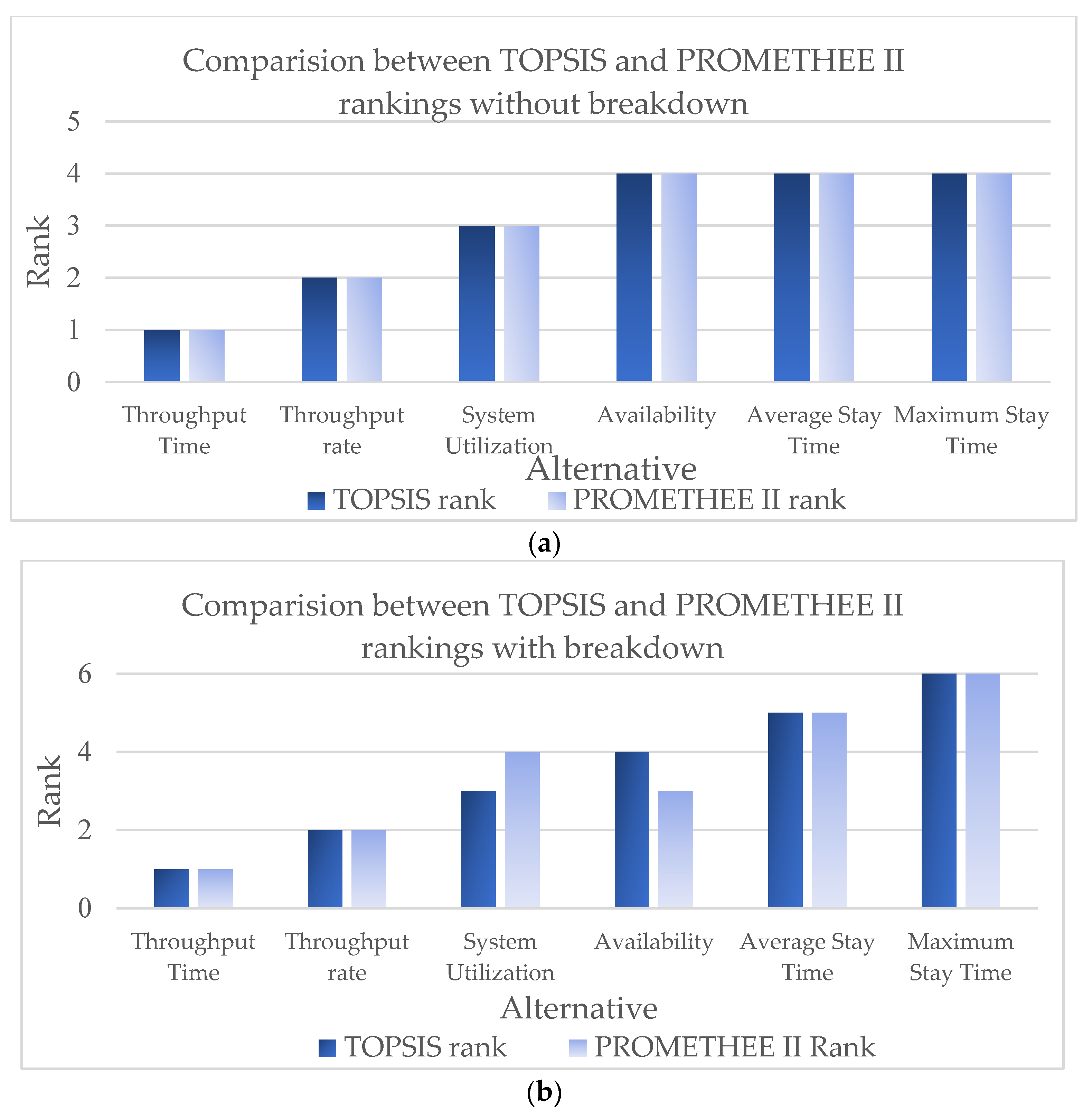
Various techniques have been applied in previous literature [15] to make decisions or rank alternatives, and a novel tool was outlined by [16] for the triple bottom line for deciding the appropriate process route by considering the various key performance indicators. It has been observed that one of the popular methods is the integrated MCDM method, but little research has been done in the field of ranking the parameters of flexible systems with the Technique of Order Preference by Similarity to the Ideal Solution (TOPSIS) method. In this paper, therefore, the Entropy method has been used for finding the weight of each criterion, and the TOPSIS method has been used for ranking parameters from the most affected to the least affected. Later, rankings obtained from TOPSIS are compared with the PROMETHEE method. The reason for using the Entropy method to find weights instead of the AHP method is that the Entropy method provides objectivity in determining the weights of an index, whereas AHP uses only subjective criteria. The limitation of the AHP method is that it only works because of the positive reciprocal matrix. Various MCDM tools, such as Simple Additive Weighting (SAW), Analytical Hierarchy Process (AHP), TOPSIS, Analytic Network Process (ANP), Elimination, Choice Translating Reality [17], and others, were proposed for the ranking of alternatives. From various literature, it has been observed that the TOPSIS method is one of the MCDM methods that can offer both quantitative and qualitative study for a particular problem, and it provides the better decisions for real-life complex situations than AHP, FAHP, and other MCDM methods [18,19,20,21,22,23]. In this paper, we try to investigate performance measures viz. throughput rate, Throughput Time, system use, Availability, average stay time, and Maximum Stay Time on different scenarios of complex manufacturing systems with varied flexibility. However, disruptions to any of the systems are most common issues. Irrespective of technological advancements, improper and delayed handling of these issues may lead to counterproductive results. Therefore, the proper choice of parameter ranking greatly impacts flexible systems regarding their performance and reliability.
Thus, this study seeks to address the following research questions:
  • Which performance parameters influence the proposed flexible configurations most and least, with and without the breakdown of machines?
  • How can system behavior in the case of normal and disruption conditions be understood?
On the whole, the contributions of this research paper are as follows:
  • Simulation analysis was conducted with the help of simulation software by varying the number of jobs from 100 to 5000 by considering cases with and without the breakdown of machines for various configurations, to compare the experimental results.
  • A validated proposed MCDM-TOPSIS-based simulation approach was taken to rank parameters to understand flexible system behavior in normal and uncertain conditions.
Thus, the above-mentioned performance measures need to be analyzed to maintain the best health status of a system. Therefore, first an integrated MCDM-TOPSIS method was used along with an Entropy method to identify the weight of each parameter and to identify the most influencing performance measure. Thereafter, with the considered process parameters, simulations are conducted to analyze performance both with disruptions and without disruption. The proposed approach is validated with real-time experimental results [9]. The results demonstrate the ability to understand the system behavior.
The remainder of this paper is organized as follows. Section 2 provides a comprehensive overview of relevant literature. Section 3 discusses the integrated MCDM-TOPSIS-based simulation methodology. Comparative results are examined in Section 4. Section 5 contains the Entropy-based TOPSIS method for simulation results. Finally, Section 6 presents conclusions and gives directions for future research.

2. Literature Review

This section offers an overview of the relevant literature on PHM of flexible machine systems and an integrated MCDM-TOPSIS method simulation approach on manufacturing systems. As manufacturing systems are disrupted due to their own natural characteristics or unexpected downtimes, health management for machines is considered to be a vital approach for better performance, as mentioned by [24,25]. Based on the mentioned problematic condition, [12,26] proposed a method to control disruptions and predict the failure time of each machine in a parallel configuration by adjusting the workloads on individual machines. This transformation has led to a lot of studies on maintenance methodologies related to manufacturing systems [27]. The health status of a machine can be evaluated by conventional prognostics and diagnostics approaches, and these are essential in the case of machine health management in Industry 4.0 [28,29].
Generally, manufacturing systems can be designed differently according to company strategy, boundary conditions, and the goals mentioned in [
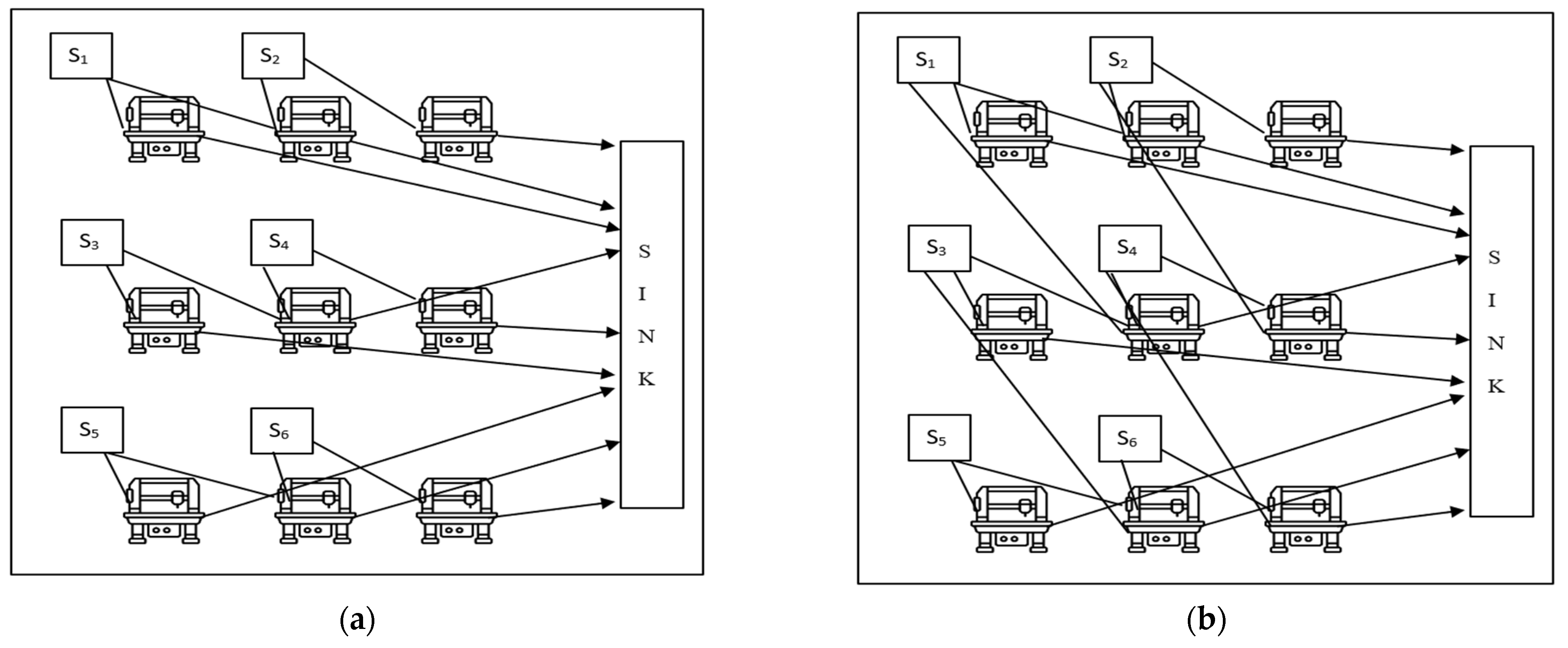
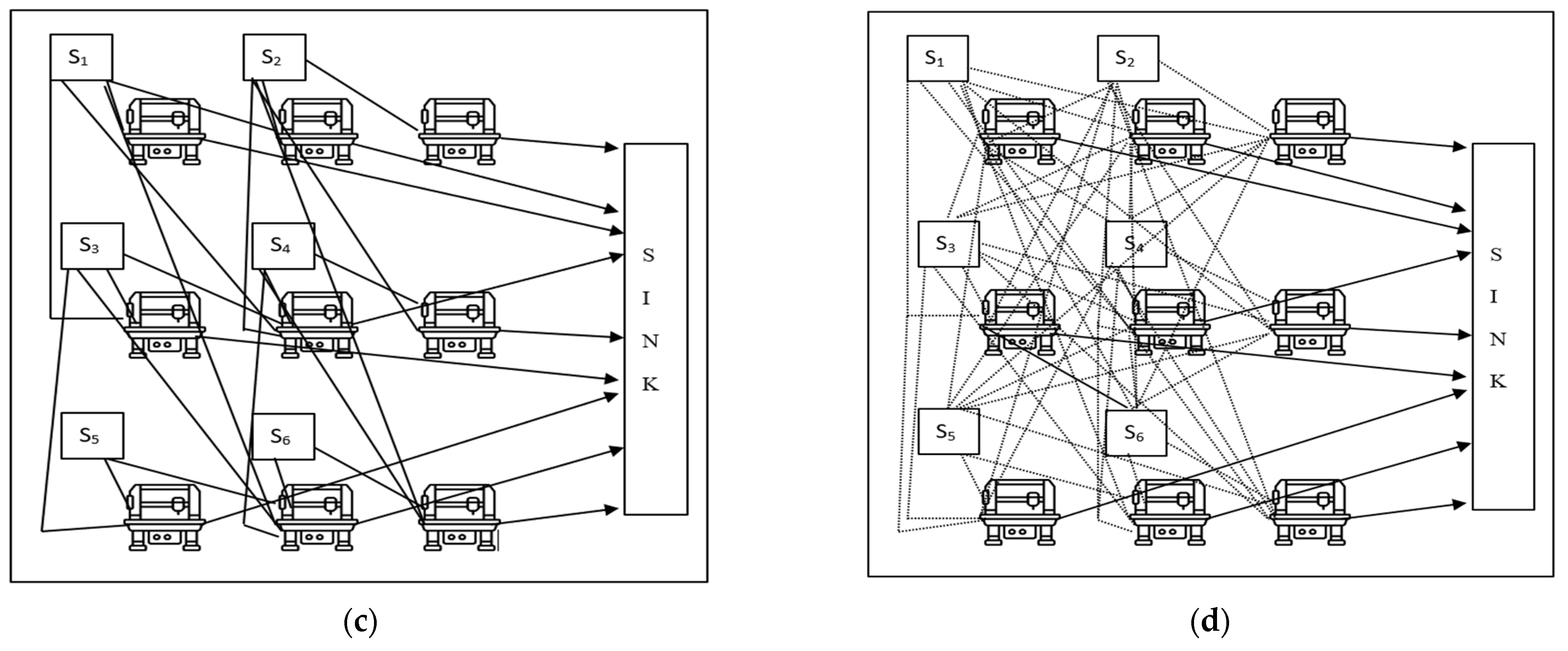
30]. Among all the existing manufacturing system configurations, semi–fully flexible real-time configurations, i.e., one-degree, two-degree, semi-flexible, and fully flexible configurations, are considered in the literature for the simulation analysis [9]. The above-mentioned configuration provides routing flexibility, so that the system can use two or more machines to perform the same task, and assess the system’s ability to handle many changes, such as a substantial increase in capacity and machine failure [31].
From the various literature [32,33], it has been shown that six performance parameters need to be considered that influence the above-mentioned four configuration performances. These parameters influence a flexible machine system performance, as machine availability can be an important determinant of the delivery speed and delivery dependability, because unexpected machine downtime will not only increase lead time but also disrupt the production plan [33]. Such disruptions can be detrimental to a Just-in-Time (JIT) manufacturing environment. Alongside that, the average stay time of jobs, Maximum Stay Time of jobs, maintenance costs, and production cost force firms to analyze the performance of their systems systematically and efficiently regarding the availability of machines [13]. Simulation analysis for these performance parameters helps with visualizing and understanding system behavior for real-time manufacturing systems mentioned by [34,35,36,37,38]. A comparison of various features of this present study with other recent studies is shown in Table 1, below.
A method needs to be used for ranking the performance parameters from most influenced to least, which furthermore can help with increasing manufacturing system performance and product quality. The integrated MCDM method considers all standards and the importance that decision-makers place to determine the most satisfactory solution based on performance evaluation [35]. Refs [35,36] mention that different MCDM techniques have been used to solve problems related to decision-making or ranking among alternatives. An Entropy method was presented by the [37] and was used in this paper for finding the weight of each criterion. An integrated MCDM methodology based on the TOPSIS method was used in this paper to rank the parameters. Among the various MCDM techniques, the TOPSIS method is best suited for decision-making problems since it has been observed that the TOPSIS method is preferred for considering the quantitative criteria mentioned by [17].
The main principle of the TOPSIS method is that the selected alternative should be the shortest distance from the positive ideal solution and the largest distance from the negative ideal solution. To determine the attribute weight for the TOPSIS method, the Entropy method is frequently used [21,22]. Generally, the Entropy method is used to calculate the weights of each criterion when decision-makers have conflicting views on the value of weights.

3. Methodology

In this paper, the performance process parameters were analyzed using the simulation analysis approach, and then the results were validated using real-time experimental calculation results. Later, an integrated MCDM method was selected to rank the parameters, because MCDM is a well-known technique for solving complex real-life problems of diverse alternatives using several criteria to rank or choose the best or worst alternative.
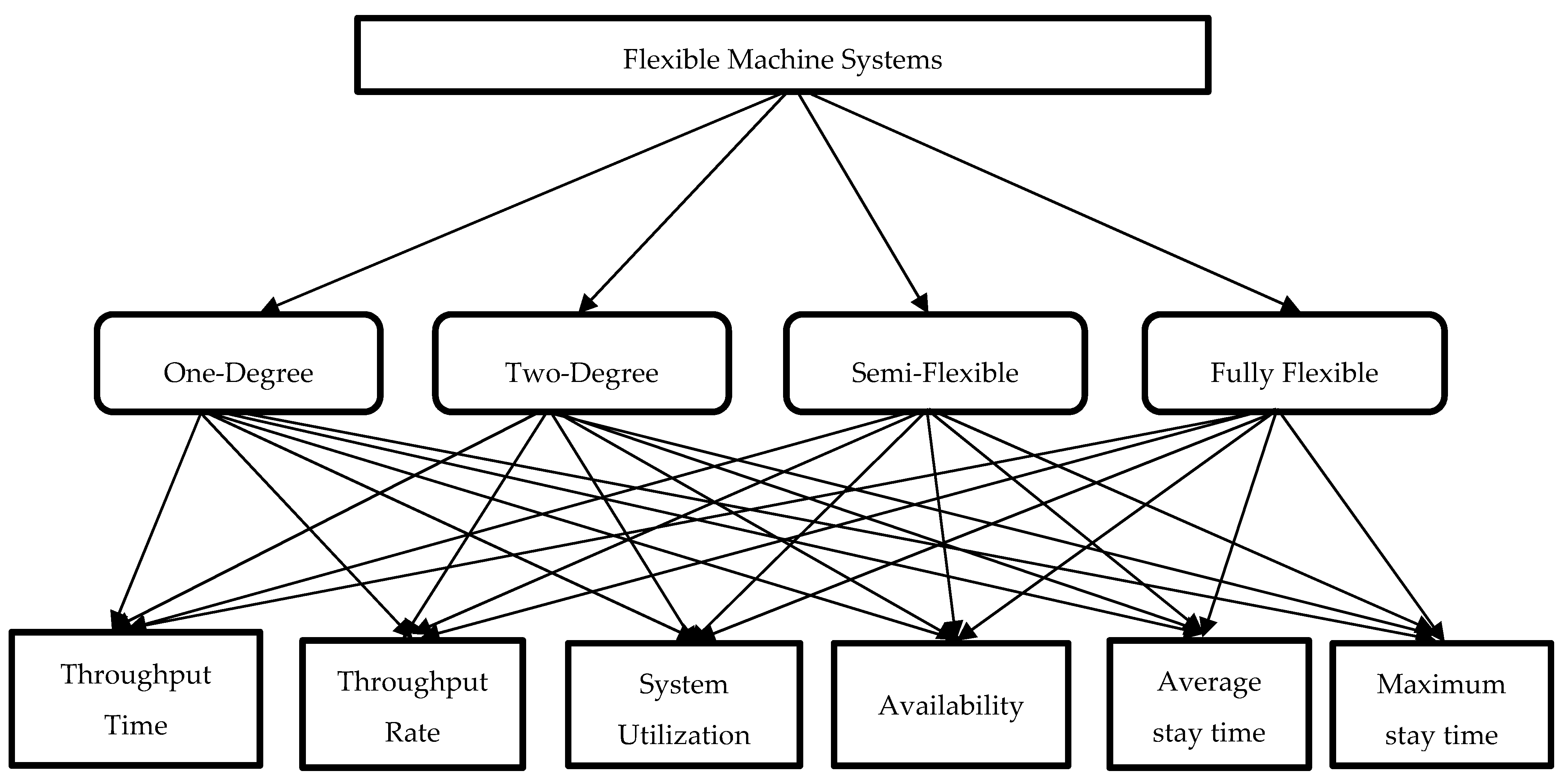
Different MCDM techniques can be used for solving decision-making problems, but TOPSIS is the best suited, and it has been observed that the TOPSIS method is preferred for considering quantitative criteria. The Entropy method is used in conjunction with the TOPSIS method. The Entropy method is applied to calculate the weight of each criterion and the TOPSIS method is used for evaluating the alternatives (parameters) based on these criteria. Various key parameters that influence flexible machine systems are shown in Figure 1, below.
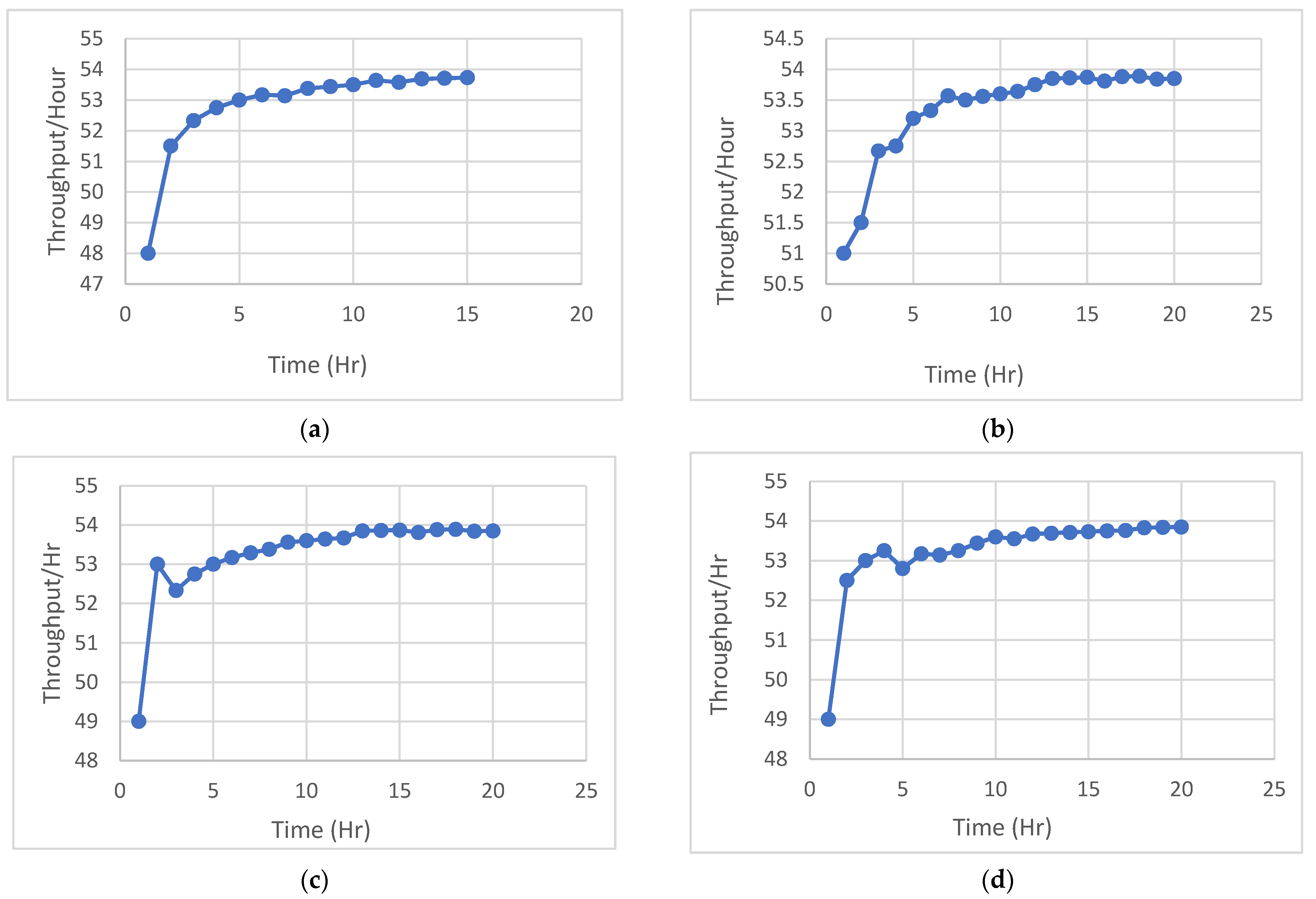
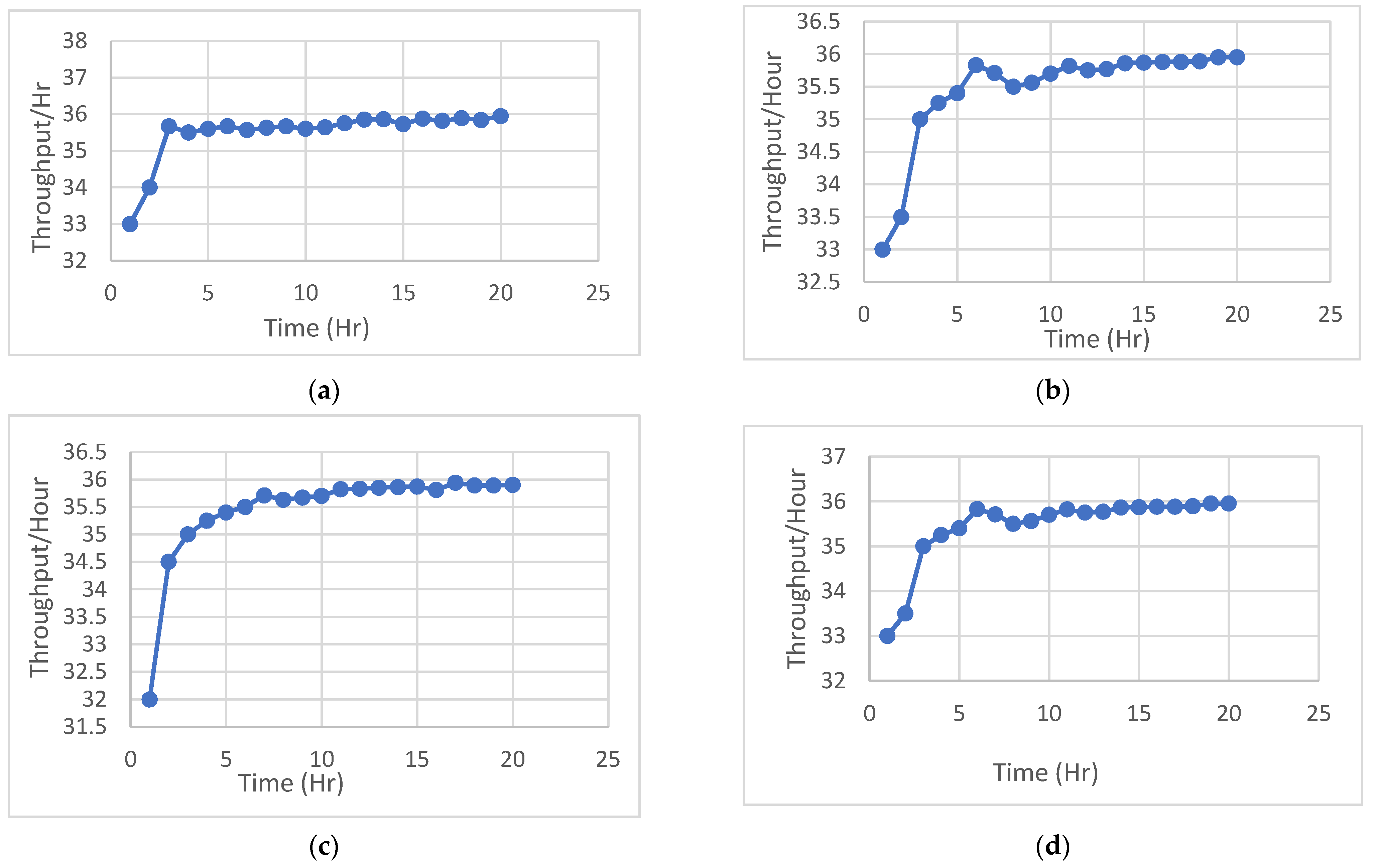
In the experimentation analysis, the number of jobs has been taken as 5000, and the values of each individual parameter have been calculated. After that, the simulation analysis was conducted with the help of simulation software by varying the number of jobs from 100 to 5000. The obtained simulation results are mostly near the experimental values. Finally, the parameters of simulation results were ranked by influence on the flexible machine systems, from most to least. 
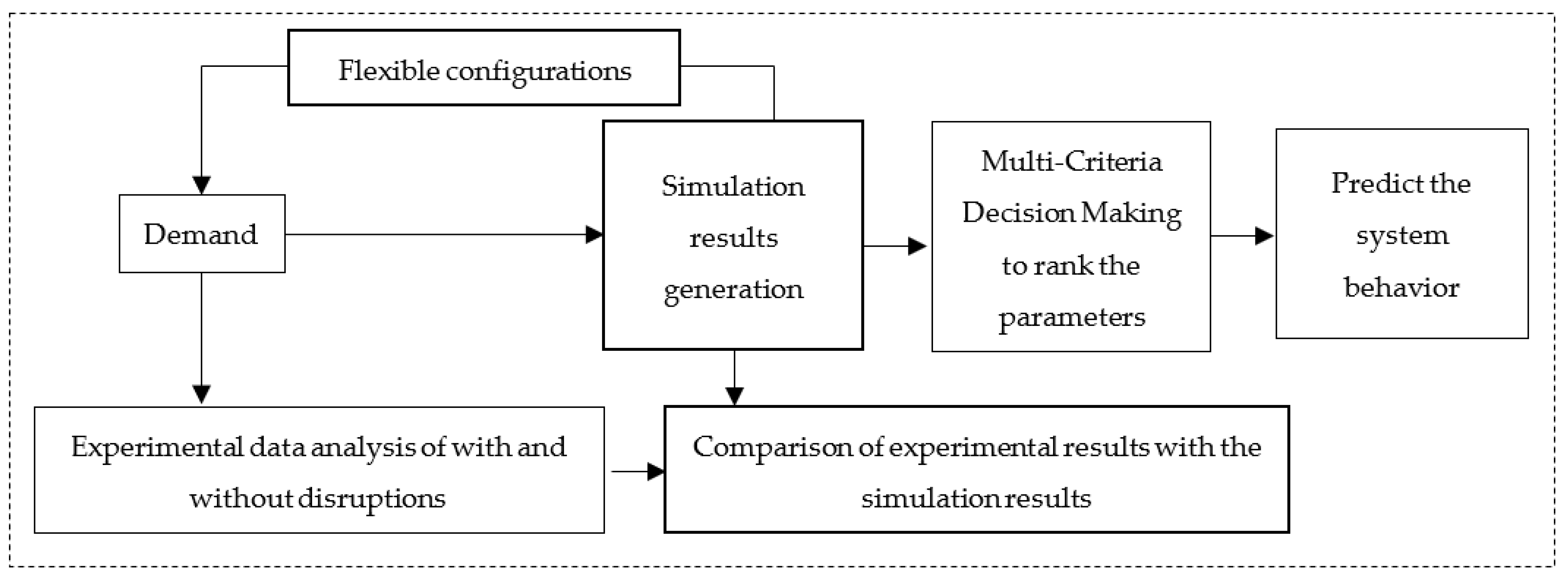
Figure 2 outlines the overview of the integrated MCDM-based simulation approach.

4. Comparative Results

Here, S1, S2… S6 indicates the sources from where jobs can be assigned to processors. The flexible machine systems consist of N number of identical machines in which the system must operate simultaneously to complete the given number of jobs shown in Figure 3. Figure 3a presents the one-degree flexible system in which, if any machine fails, then the remaining number of jobs can be adjusted on an adjacent connected machine. Figure 3b represents the two-degree flexible system in which, if any machine fails, then the remaining number of jobs can be adjusted on two adjacent connected machines depending upon the availability of machines. Here, the availability of machines has been increased in the case of two-degree flexible configuration compared to one-degree flexible configuration. Figure 3c,d represents the semi-flexible and fully flexible machines, in which the availability of machines is more compared to the one-degree flexible system than the two-degree flexible system [9].

4.1. Experimental Analysis

The values of each parameter have been calculated by considering the number of jobs as 5000 and, as mentioned below in Table 2, to obtain that level a majority of machines break down at least once. Throughput time is the actual time taken to manufacture a product, and it can be calculated by multiplying the average stay time by the total number of jobs per machine compared with the existing literature values [9]; similarly, throughput rate is the rate at which units move from start to finish, and it can be calculated by dividing the output by the Throughput Time. The Availability is the amount of time in which the machine runs and is available for production, and can be calculated by Equation (1).
A v a i l a b i l i t y = M T B F M T B F + M T T R
The average stay time and Maximum Stay Time can be calculated from the bell curve by considering a 99.97% confidence level since the processing time follows the normal distribution. The system use can be defined as the proportion of time that the manufacturing system is used, and system use is calculated by Equation (2).
U t i l i z a t i o n = A c t u a l   O u t p u t M a x i m u m   L e v e l   O u t p u t

4.2. Simulation Analysis

Simulation analysis was conducted on a PC with Intel Corei3-7100 U (2.40 GHz) running on the Windows 10 Professional operating system with 8 GB of RAM. The images of various configurations from a single degree to fully flexible are shown in Figure 3. The processing time, mean time between failures (MTBF), and Mean Time to Repair (MTTR) follow the normal distribution, and the time required to repair a machine has been considered to be constant.

4.2.1. Warm-Up Period

The number of replications for the simulation was determined as 20 and the length of each replication was 1 h with a warm-up period of 8 h for a one-degree flexible configuration, as shown in Figure 4a in the case of no breakdown of machines. The warm-up period for the two-degree flexible configuration, semi-flexible, and fully flexible configurations without the breakdown of machines are 8 h, 13 h, and 10 h, as shown in Figure 4b–d, respectively. Similarly, the warm-up period with the breakdown of machines for various configurations is shown in Figure 5. The warm-up period for one-degree and two-degree flexible configuration, semi-flexible, and fully flexible configurations following the breakdown of machines are 6 h, 14 h, 11 h, and 14 h as shown in Figure 5a–d, respectively. The warm-up period has been obtained by applying Welch’s procedure [38] to estimate a steady-state mean. The technique often suggested for these kinds of problems is called the warm-up period or initial data deletion. The main idea is to delete the initial observations from the run and use the remaining observations to obtain the steady state. The number of replications has been calculated with the help of the following Equation (3) [38].
X ¯ ( n ) ± t n 1 , 1 α / 2 s n
where X ¯ ( n ) represents the sample mean, s represents sample standard deviation, and n represents the number of replications, and t n 1 , 1 α / 2 is the upper and 1 α / 2 critical points where the warm-up period is in the case of breakdown for one-degree configuration of 6 h. Then, the desired confidence interval for 95% confidence level is 6 ± t 19 , 0.025 7.504 20 . From the results, it can be observed that the 20 simulations are enough from the initial approach mentioned in [38]. The warm-up period has been identified from the plot as shown in the figure below for various configurations.

4.2.2. Parameter Analysis

Various parameters, such as Throughput Rate (TR) in throughput/hour, Throughput Time (TT) in seconds, System Use (SU) as a percentage, Availability (A), Average Stay Time (Tavg) in seconds, Maximum Stay Time (Tmax) in seconds, have been generated with the help of simulation software for one-degree, two-degree, semi-flexible, and fully flexible configurations without and with the breakdown of machines. The number of machines has been varied from 100 to 5000, and the simulation results have been presented for various configurations in Table 3, Table 4, Table 5 and Table 6, respectively.
The collected values of the parameters’ effect on flexible machine systems are represented in Table 7. These values were generated using the simulation procedure for various configurations without and with machine breakdown by considering the number of jobs as 5000. Initially, different normally distributed Mean Time Between Failure (MTBF) values for the different machines (processors) and constant MTTR (Mean Time to Repair) as 1 day and normally distributed processing time has been considered to obtain random failure.
Figure 6A–D represents the simulation results of various parameters (throughput rate, system use, and average stay time) for various configurations without the breakdown of machines. Similarly, Figure 7A–D represents the simulation results of the above-mentioned parameters with the breakdown of machines. These simulation results have been generated by arranging the machines as per the configuration and data have been provided in the simulation software with the help of MTBF, MTTR, and processing time for each machine.

5. Proposed Entropy Weight-Based TOPSIS Method

In this paper, the frequently used normalization methods Entropy and TOPSIS methods, as these two methods are used in combination with each other, have been analyzed for the collected simulation data. The Entropy method is used to calculate the weights of each criterion when decision-makers have conflicting views. The weights calculated by the Entropy method are also called objective weights. The Entropy method shows how much different alternatives approach one another in respect to a certain criterion. The best advantage of the Entropy method is the avoidance of human factor interference on the weights of indicators. With this advantage, the Entropy method has been widely used in recent years. The Entropy method consists of four steps, as mentioned below. Equations (4)–(7) are formulas to calculate the weights of each criterion are as follows [21,22]. The TOPSIS method is used to find a ranking for each individual alternative. The TOPSIS method is used to obtain the solution which is nearest the positive ideal solution and farthest from the negative ideal solution. The application of the TOPSIS method in ranking various factors that affect flexible unit systems has been reported in the literature. Various steps involved in the TOPSIS method are explained below with the help of Equations (8)–(14) [21,22].

5.1. Weight Calculation by Entropy Method

  • Step 1. Normalize the decision matrix
The performance value of a t h alternative and b t h criteria in Equation (4) is indicated by A a b = ( a = 1 , 2 , , m ; b = 1 , 2 , , n ) and the normalized matrix is shown in Table 8.
B a b = u a b a = 1 m u
  • Step 2. Entropy value of E b for b t h criteria
Entropy value E j of b t h criteria can be obtained by Equation (5) and is shown in Table 9.
E b = K   a = 1 x B a b   ln ( B a b )             b = 1 , 2 , , x
where K = 1 / ln x is a constant to satisfy the condition 0 E b 1 and ‘ b ’ indicates the number of alternatives or factors.
  • Step 3. The degree of divergence of average information
The degree of divergence of average needs to be discovered using Equation (6). The degree of diversity value matrix is calculated and shown in Table 10.
D b = | 1 E b |
  • Step 4. The weight of Entropy of b’th criteria
The weight of criterion can be calculated by Equation (7) and is represented in Table 11.
B b = D b b = 1 y D b

5.2. Ranking the Parameters by TOPSIS Method

  • Step 1. Normalization of the decision matrix.
The normalization matrix can be calculated by Equation (8). The normalized decision matrix is formed and shown in Table 12.
N a b = u a b a = 1 x u 2         b = 1 , 2 , y ;         a = 1 , 2 , , x ;
  • Step 2. Construct the weighted normalized decision matrix.
The associated weights W b are multiplied with the normalized matrix and taken from each parameter to be obtained by following Equation (9). The weighted normalized decision matrix is formed and shown in Table 13.
V a b = N a b W b           b = 1 , 2 , y           a = 1 , 2 , x
  • Step 3. Determining positive ideal solution and negative ideal solution.
The positive ideal solution and the negative ideal solution are determined using Equations (10) and (11) respectively. The positive ideal and negative ideal solution matrix is formed and shown in Table 14.
{ V 1 + , V 2 + , , V n + } = { ( M a x   V a b | b K ) , ( M i n   V a b | b K | ) |         a = 1 , 2 , , x }
{ V 1 , V 2 , , V n } = { ( M i n   V a b | b K ) , ( M a x   V a b | b K | ) |         a = 1 , 2 , , x }
where K is the index of set of benefit criteria and K | is the index of cost criteria.
  • Step 4. Finding the Euclidean distance from positive ideal solution and negative ideal solution.
The Euclidean distance from positive ideal solution and negative ideal solution can be computed by the below Equations (12) and (13), respectively. The Euclidian distance matrix from positive ideal solution and negative ideal solution is formed and shown in Table 15.
S i + = { b = 1 y ( V a b V b + ) 2 } 1 / 2         b = 1 , 2 , y ;         a = 1 , 2 , , x ;
S i = { b = 1 y ( V a b V b ) 2 } 1 / 2         b = 1 , 2 , y ;         a = 1 , 2 , , x ;
  • Step 5. Calculating the relative closeness (performance score).
The relative closeness is calculated from the ideal solution using Equation (14).
C i = S i S i + + S i         a = 1 , 2 , , x ;     0 C i 1
Equation (14) indicates the relative closeness in which the higher value indicates the best rank and lower value indicates the worst rank. The relative closeness value matrix is formed based on obtained value, and ranks the parameters as shown in Table 16.

5.3. Ranking the Parameters by PROMETHEE II Method

PROMETHEE (Preference Ranking Organization Method for Enrichment Evaluations) is a MCDM method, and it has been widely used to rank the alternatives in many decision-making problems [39]. This method is based on a pair to pair of possible decisions along with each criterion. Various possible decisions need to be evaluated according to different criteria, which is to be maximized or minimized.
  • Step 1. Determination of pairwise comparisons deviations. It can be calculated by Equation (15).
    d j ( m , n ) = g j ( m ) g j ( n )
    where d j ( m , n ) is the difference between the evaluations of m , n on each criterion.
  • Step 2. Application of preference function is shown in Equation (16).
    S j ( m , n ) = F j [ d j ( m , n ) ]             j = 1 , 2 , , k
    where S j ( m , n ) indicates the preference of alternative m with regard n on each criterion.
  • Step 3. Calculation of global preference index can be calculated by Equation (17).
    m , n A ,             π ( m , n ) = j = 1 k P j ( m , n ) w j
    where π ( m , n ) defined as the weighted sum of each criterion, w j denotes the weight associated with the j’th criterion.
  • Step 4. Calculation of outranking flows can be calculated by Equation (18).
    ϕ + ( a ) = 1 x 1 y A π ( m , y )       and       ϕ ( a ) = 1 n 1 y A π ( y , m )
    where ϕ + ( a ) , ϕ ( a ) indicates positive outranking flow and negative outranking flow for each alternative.
  • Step 5. Calculation of net outranking flow can be calculated by Equation (19).
    ϕ ( a ) = ϕ + ( a ) ϕ ( a )
    where ϕ ( a ) indicates the net outranking flow.
The comparison between the TOPSIS and PROMETHEE II rankings without breakdown and with a breakdown of machines is shown in below Table 17, and the comparison between the TOPSIS and PROMETHEE II rankings without breakdown and with breakdown plots is shown in Figure 8a,b.

6. Conclusions and Future Directions

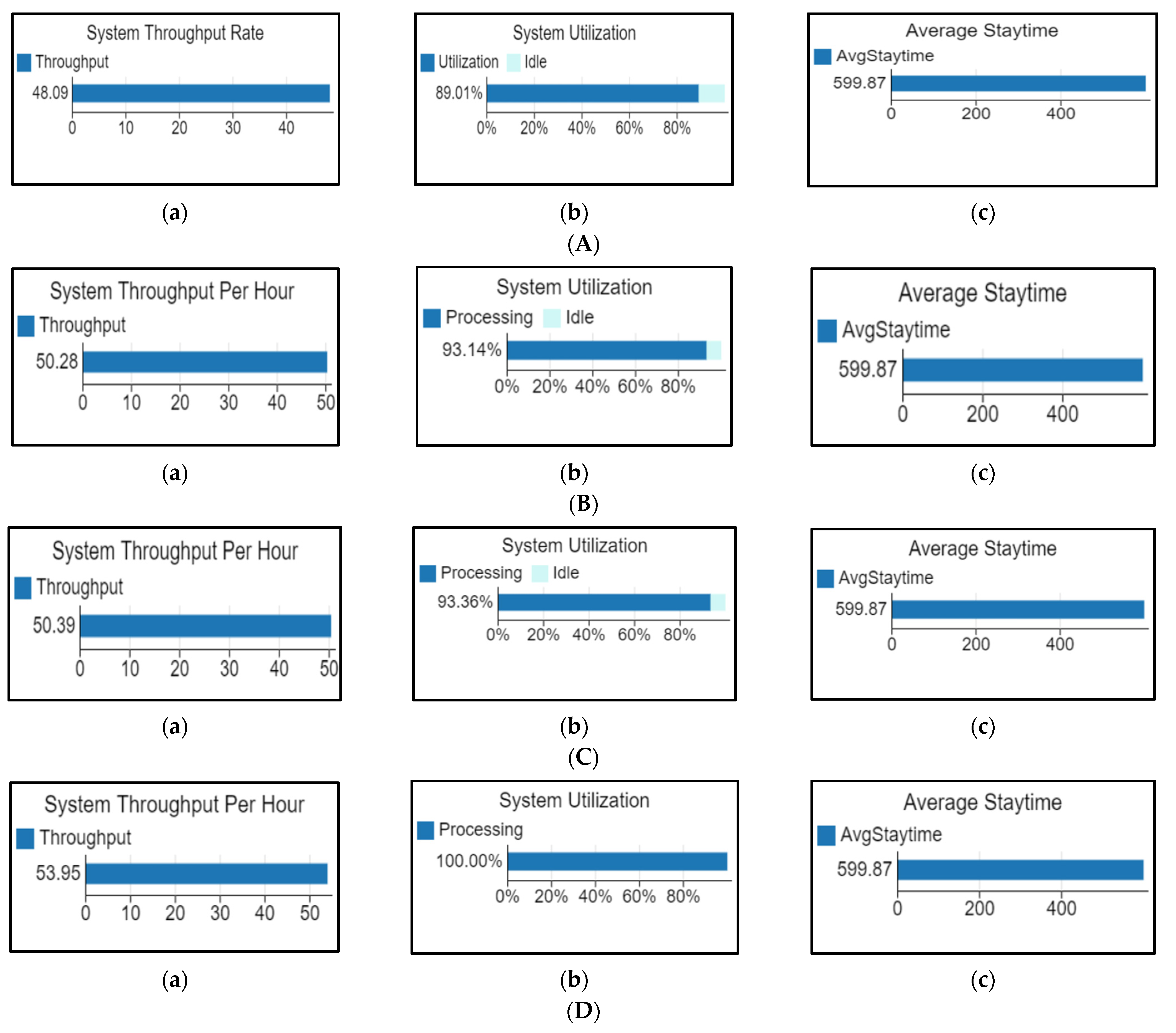
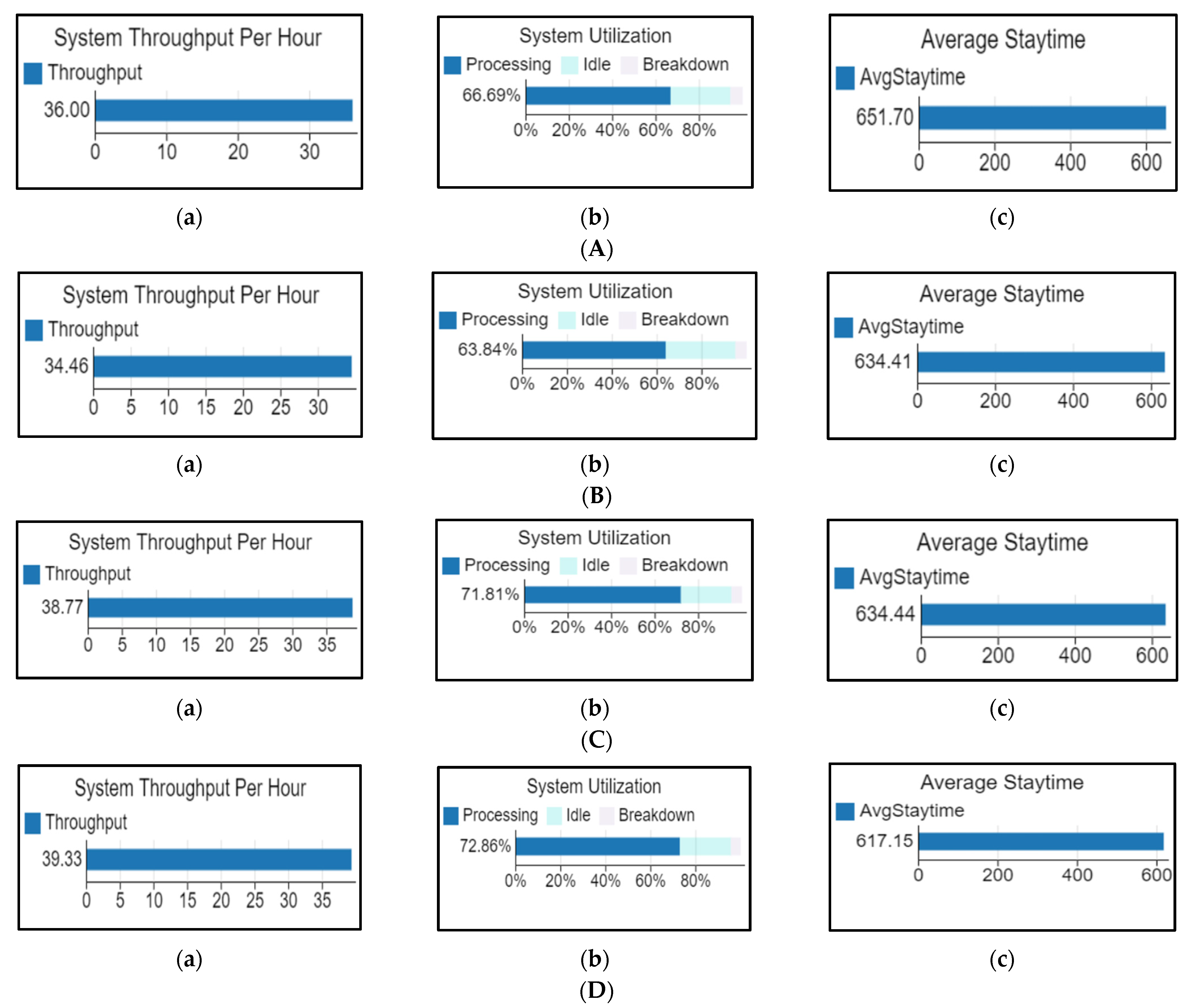
In this paper, the maximum number of jobs has been taken as 5000 in a real-time experiment and values of mentioned six parameters, i.e., throughput rate, Throughput Time, system use, Availability of machines, average stay time, and Maximum Stay Time, have been obtained. To compare these experimental results, simulation analysis was conducted with the help of simulation software by varying the number of jobs from 100 to 5000 by considering the breakdown of machines and no breakdown for various configurations. Later, the Entropy method was used for simulation results to compute the weights of each criterion, and the integrated MCDM-TOPSIS method was employed to rank the parameters from the most affected to the least affected by considering breakdown and no breakdown of machines. From the obtained results, it can been observed that the Throughput Time of 431,921.51 s is the most affected performance parameter and Availability, Average Stay Time, and the Maximum Stay Time of 1599.87 s and 712.62 s, respectively, are the least affected performance parameters without the breakdown of machines. Throughput Time of 521,598.36 s is the most affected performance parameter and Maximum Stay Time of 87,012.33 s is the least affected performance parameter in the case of the breakdown of machines condition for a one-degree flexible configuration. Similarly, in the case of a two-degree flexible configuration, the Throughput Time of 386,801.83 s is the most affected parameter and Availability, Average Stay Time and the Maximum Stay Time of 1599.87 s and 712.62 s, respectively, are the least affected parameters without breakdown, and the same values with breakdown condition. Similarly, in the semi-flexible configuration, the most and least influenced parameters are Throughput Time of 403,983.15 s and Availability of 1, Average Stay Time of 599.87 s, and Maximum Stay Time of 712.62 s, which are the least affected parameters without breakdown. Throughput Time of 503,929.54 s is most affected and 87,010.2 s is least affected in the case of the breakdown condition. Similarly, in the case of fully flexible configuration, the Throughput Time of 369,613.81 s is the most affected and Availability of 1, Average Stay Time of 599.87 s, and Maximum Stay Time of 712.62 s are the least affected parameters without breakdown, and the Throughput Time of 508,033.76 s as most affected and 87,037.7 s as least affected in the case of the breakdown condition. In the future, the proposed methodology can help firm management to take verdicts refining the performance parameters of various proposed flexible systems and understand the manufacturing system behavior and its influencing parameters in normal and various uncertain conditions.

Author Contributions

Conceptualization, V.K.M. and T.S.; methodology, T.S. and S.K.; software, S.K. and T.S.; validation, T.S., V.K.M., S.K. and J.M.; formal analysis, T.S. and S.K.; investigation, V.K.M. and K.A.; resources, T.S. and J.M.; data curation, V.K.M. and S.K.; writing—original draft preparation, T.S. and V.K.M.; writing—review and editing, V.K.M., J.M. and K.A.; visualization, S.K. and J.M.; supervision, V.K.M., J.M. and K.A.; project administration, V.K.M.; funding acquisition, V.K.M. and J.M. All authors have read and agreed to the published version of the manuscript.

Funding

This work has been, also, supported by the FCT within the RD Units Project Scope: UIDP/04077/2020 and UIDB/04077/2020.

Acknowledgments

The authors thank the Department of Production and Systems from University of Minho and the FCT-Fundação para a Ciência e Tecnologia, both from Portugal.

Conflicts of Interest

The authors declare no conflict of interest.

References

  1. Calabrese, F.; Regattieri, A.; Botti, L.; Galizia, F.G. Prognostic health management of production systems. New proposed approach and experimental evidences. Procedia Manuf. 2019, 39, 260–269. [Google Scholar] [CrossRef]
  2. Pellegrino, J.; Justiniano, M.; Raghunathan, A.; Weiss, B.A. Measurement Science Roadmap for Prognostics and Health Management for Smart Manufacturing Systems; NIST: Gaithersburg, MD, USA, 2016. [Google Scholar] [CrossRef]
  3. Kaur, G.; Yadav, R.; Majumder, A. An efficient intuitionistic fuzzy approach for location selection to install the most suitable energy power plant. In Proceedings of the 2nd International Conference on Recent Advances in Fundamental and Applied Sciences RAFAS (2019), Punjab, India, 5–6 November 2019; IOP Publishing: Bristol, UK, 2020; Volume 1531, p. 012057. [Google Scholar] [CrossRef]
  4. Dey, B.K.; Bhuniya, S.; Sarkar, B. Involvement of controllable lead time and variable demand for a smart manufacturing system under a supply chain management. Expert Syst. Appl. 2021, 184, 115464. [Google Scholar] [CrossRef]
  5. Nandra, R.; Majumder, A.; Mishra, M. A multi-retailer sustainable supply chain model with information sharing and quality deterioration. RAIRO-Oper. Res. 2021, 55, S2773–S2794. [Google Scholar] [CrossRef]
  6. Dey, B.K.; Pareek, S.; Tayyab, M.; Sarkar, B. Autonomation policy to control work-in-process inventory in a smart production system. Int. J. Prod. Res. 2021, 59, 1258–1280. [Google Scholar] [CrossRef]
  7. Aghaie, M.; Fazli, S. An improved MCDM method for maintenance approach selection: A case study of auto industry. Manag. Sci. Lett. 2012, 2, 137–146. [Google Scholar] [CrossRef]
  8. Emovon, I.; Oghenenyerovwho, O.S. Application of MCDM method in material selection for optimal design: A review. Results Mater. 2020, 7, 100115. [Google Scholar] [CrossRef]
  9. Samala, T.; Manupati, V.K.; Nikhilesh, B.B.S.; Varela, M.L.R.; Putnik, G. Job adjustment strategy for predictive maintenance in semi-fully flexible systems based on machine health status. Sustainability 2021, 13, 5295. [Google Scholar] [CrossRef]
  10. Hao, L.; Gebraeel, N.; Shi, J. Simultaneous signal separation and prognostics of multi-component systems: The case of identical components. IIE Trans. 2015, 47, 487–504. [Google Scholar] [CrossRef]
  11. Li, H.; Parlikad, A.K. Study of dynamic workload assignment strategies on production performance. IFAC-PapersOnLine 2017, 50, 13710–13715. [Google Scholar] [CrossRef]
  12. Manupati, V.K.; Panigrahi, S.; Ahsan, M.; Lahiri, S.; Chandra, A.; Thakkar, J.J.; Putnik, G.; Varela, M.L.R. Estimation of manufacturing systems degradation rate for residual life prediction through dynamic workload adjustment. Sādhanā 2019, 44, 30. [Google Scholar] [CrossRef] [Green Version]
  13. Swamidass, P.M. (Ed.) Encyclopedia of Production and Manufacturing Management; Springer Science & Business Media: Berlin/Heidelberg, Germany, 2000. [Google Scholar] [CrossRef]
  14. Lugaresi, G.; Alba, V.V.; Matta, A. Lab-scale models of manufacturing systems for testing real-time simulation and production control technologies. J. Manuf. Syst. 2021, 58, 93–108. [Google Scholar] [CrossRef]
  15. Tan, T.; Mills, G.; Papadonikolaki, E.; Liu, Z. Combining multi-criteria decision making (MCDM) methods with building information modelling (BIM): A review. Autom. Constr. 2021, 121, 103451. [Google Scholar] [CrossRef]
  16. Saxena, P.; Stavropoulos, P.; Kechagias, J.; Salonitis, K. Sustainability assessment for manufacturing operations. Energies 2020, 13, 2730. [Google Scholar] [CrossRef]
  17. Rouyendegh, B.D.; Erol, S. Selecting the best project using the fuzzy ELECTRE method. Math. Probl. Eng. 2012, 2012, 790142. [Google Scholar] [CrossRef]
  18. Afshari, A.; Mojahed, M.; Yusuff, R.M. Simple additive weighting approach to personnel selection problem. Int. J. Innov. Manag. Technol. 2010, 1, 511–515. [Google Scholar] [CrossRef]
  19. Kumar, R.; Ray, A. Selection of material for optimal design using multi-criteria decision making. Procedia Mater. Sci. 2014, 6, 590–596. [Google Scholar] [CrossRef] [Green Version]
  20. Opricovic, S.; Tzeng, G.H. Compromise solution by MCDM methods: A comparative analysis of VIKOR and TOPSIS. Eur. J. Oper. Res. 2004, 156, 445–455. [Google Scholar] [CrossRef]
  21. Ding, L.; Shao, Z.; Zhang, H.; Xu, C.; Wu, D. A comprehensive evaluation of urban sustainable development in China based on the TOPSIS-entropy method. Sustainability 2016, 8, 746. [Google Scholar] [CrossRef] [Green Version]
  22. Kaynak, S.; Altuntas, S.; Dereli, T. Comparing the innovation performance of EU candidate countries: An entropy based TOPSIS approach. Econ. Res.-Ekon. Istraživanja 2017, 30, 31–54. [Google Scholar] [CrossRef]
  23. Khan, W.U.; Ali, M. Effect of routing flexibility on the performance of manufacturing system. Int. J. Prod. Manag. Eng. 2019, 7, 133–144. [Google Scholar] [CrossRef] [Green Version]
  24. Alexandru, A.M.; De Mauro, A.; Fiasché, M.; Sisca, F.G.; Taisch, M.; Fasanotti, L.; Grasseni, P. A smart web-based maintenance system for a smart manufacturing environment. In Proceedings of the 2015 IEEE 1st International Forum on Research and Technologies for Society and Industry Leveraging a Better Tomorrow (RTSI), Turin, Italy, 16–18 September 2015; IEEE: Manhattan, NY, USA; pp. 579–584. [Google Scholar] [CrossRef] [Green Version]
  25. Samala, T.; Manupati, V.K.; Varela, M.L.R.; Putnik, G. Investigation of Degradation and Upgradation Models for Flexible Unit Systems: A Systematic Literature Review. Future Internet 2021, 13, 57. [Google Scholar] [CrossRef]
  26. Hao, L.; Liu, K.; Gebraeel, N.; Shi, J. Controlling the residual life distribution of parallel unit systems through workload adjustment. IEEE Trans. Autom. Sci. Eng. 2015, 14, 1042–1052. [Google Scholar] [CrossRef]
  27. Ajukumar, V.N.; Gandhi, O.P. Evaluation of green maintenance initiatives in design and development of mechanical systems using an integrated approach. J. Clean. Prod. 2013, 51, 34–46. [Google Scholar] [CrossRef]
  28. Lee, G.Y.; Kim, M.; Quan, Y.J.; Kim, M.S.; Kim, T.J.Y.; Yoon, H.S.; Min, S.; Kim, D.H.; Mun, J.W.; Oh, J.W.; et al. Machine health management in smart factory: A review. J. Mech. Sci. Technol. 2018, 32, 987–1009. [Google Scholar] [CrossRef]
  29. Lee, J.; Bagheri, B.; Kao, H.A. A cyber-physical systems architecture for industry 4.0-based manufacturing systems. Manufacturing 2015, 3, 18–23. [Google Scholar] [CrossRef]
  30. Lafou, M.; Mathieu, L.; Pois, S.; Alochet, M. Manufacturing system configuration: Flexibility analysis for automotive mixed-model assembly lines. IFAC-PapersOnLine 2015, 48, 94–99. [Google Scholar] [CrossRef]
  31. Chan, F.T. The effects of routing flexibility on a flexible manufacturing system. Int. J. Comput. Integr. Manuf. 2001, 14, 431–445. [Google Scholar] [CrossRef]
  32. Lopes, I.D.S.; Figueiredo, M.; Sá, V. Criticality evaluation to support maintenance management of manufacturing systems. Int. J. Ind. Eng. Manag. 2020, 11, 3–18. [Google Scholar] [CrossRef]
  33. Shagluf, A.; Longstaff, A.P.; Fletcher, S. Maintenance strategies to reduce downtime due to machine positional errors. In Proceedings of the Maintenance Performance Measurement and Management (MPMM) Conference 2014, Coimbra, Portugal, 4–5 September 2014; Imprensa da Universidade de Coimbra: Coimbra, Portugal, 2014. [Google Scholar] [CrossRef] [Green Version]
  34. Law, A.M.; Kelton, W.D. Simulation Modeling and Analysis; McGraw-Hill: New York, NY, USA, 2000; Volume 3. [Google Scholar] [CrossRef]
  35. Kazimieras Zavadskas, E.; Antucheviciene, J.; Chatterjee, P. Multiple-criteria decision-making (MCDM) techniques for business processes information management. Information 2019, 10, 4. [Google Scholar] [CrossRef] [Green Version]
  36. Khan, S.A.; Chaabane, A.; Dweiri, F.T. Multi-criteria decision-making methods application in supply chain management: A systematic literature. In Multi-Criteria Methods and Techniques Applied to Supply Chain Management; IntechOpen: London, UK, 2018; Volume 1. [Google Scholar] [CrossRef] [Green Version]
  37. Chodha, V.; Dubey, R.; Kumar, R.; Singh, S.; Kaur, S. Selection of industrial arc welding robot with TOPSIS and Entropy MCDM techniques. Mater. Today Proc. 2021. [Google Scholar] [CrossRef]
  38. Mavi, R.K.; Zarbakhshnia, N.; Khazraei, A. Bus rapid transit (BRT): A simulation and multi criteria decision making (MCDM) approach. Transp. Policy 2018, 72, 187–197. [Google Scholar] [CrossRef]
  39. Supraja, S.; Kousalya, P. A comparative study by AHP and TOPSIS for the selection of all round excellence award. In Proceedings of the 2016 International Conference on Electrical, Electronics, and Optimization Techniques (ICEEOT), Chennai, India, 3–5 March 2016; IEEE: Manhattan, NY, USA; pp. 314–319. [Google Scholar] [CrossRef]
  40. Dehdasht, G.; Ferwati, M.S.; Zin, R.M.; Abidin, N.Z. A hybrid approach using entropy and TOPSIS to select key drivers for a successful and sustainable lean construction implementation. PLoS ONE 2020, 15, e0228746. [Google Scholar] [CrossRef] [PubMed]
  41. Mukhamet, T.; Kobeyev, S.; Nadeem, A.; Memon, S.A. Ranking PCMs for building façade applications using multi-criteria decision-making tools combined with energy simulations. Energy 2021, 215, 119102. [Google Scholar] [CrossRef]
Figure 1. Key parameters used for the flexible machine systems.
Electronics 11 00233 g001
Figure 2. Overview of an integrated MCDM-based simulation approach.
Electronics 11 00233 g002
Figure 3. Flexible-configuration machine systems. (a) One-degree flexible system. (b) Two-degree flexible system. (c) Semi-flexible system. (d) Fully flexible system.
Electronics 11 00233 g003aElectronics 11 00233 g003b
Figure 4. Plot of output to identify the warm-up period without breakdown of machines. (a) One degree. (b) Two degrees. (c) Semi-flexible. (d) Fully flexible.
Electronics 11 00233 g004
Figure 5. Plot of output to identify the warm-up period with the breakdown of machines. (a) One degree. (b) Two degrees. (c) Semi-flexible system. (d) Fully flexible system.
Electronics 11 00233 g005
Figure 6. Simulation results by without breakdown of machines. (A) One-Degree Flexible System. (a) System Throughput rate. (b) System Use. (c) Average stay time. (B) Two-Degree Flexible System. (a) System Throughput rate. (b) System Use. (c) Average stay time. (C) Semi-Flexible System. (a) System Throughput rate. (b) System Use. (c) Average stay time. (D) Fully Flexible System. (a) System Throughput rate. (b) System Use. (c) Average stay time.
Electronics 11 00233 g006
Figure 7. Simulation results with breakdown of machines. (A) One-Degree Flexible System. (a) System Throughput rate. (b) System Use. (c) Average stay time. (B) Two-Degree Flexible System. (a) System Throughput rate. (b) System Use. (c) Average stay time. (C) Semi-Flexible System. (a) System Throughput rate. (b) System Use. (c) Average stay time. (D) Fully Flexible System. (a) System Throughput rate. (b) System Use. (c) Average stay time.
Electronics 11 00233 g007
Figure 8. (a) Ranking comparison between TOPSIS and PROMETHEEE II method without breakdown. (b) Ranking comparison between TOPSIS and PROMETHEEE II method without breakdown.
Electronics 11 00233 g008
Table 1. Comparison of features of the present review with the latest studies.
ContributorsProblemMethod UsedFeatures
Ding et al. (2016) [21]Evolution of Urban Sustainable development in ChinaTOPSIS-EntropyEvaluated the sustainable development level of 287 cities at prefecture level in China.
Supraja et al. (2016) [39]Selection of a branch of studentsAHP and TOPSISThe decisions obtained by the AHP and TOPSIS methods has been compared.
Kaynak et al. (2017) [22]Comparing the innovation performance of EU candidate countriesEntropy-based TOPSIS methodThe results of proposed methodology provides the same ranking as innovation union scoreboard and KAM.
Khan et al. (2019) [23]Simulation of routing flexibility enabled manufacturing systemsSimulation approach for finding the values of parametersEvaluated the performance measures of routing flexibility enabled manufacturing systems such as make-span time, resource use, and work in process.
Dehdasht et al. (2020) [40]The essential drivers within three aspects of sustainabilityEntropy weighted TOPSISProposed method is an effective and accurate that could help in making better decisions.
Mukhamet et al. (2020) [41]Ranking Phase Change Materials (PCMs)Combination of AHP-TOPSIS and Fuzzy AHP-Modified Fuzzy TOPSIS methodsPresented the methodology for ranking PCMs based on AHP-TOPSIS and fuzzy AHP-modified fuzzy TOPSIS methods.
Kaur et al. (2020) [3]Finding the best location for energy plant installationIntuitionistic fuzzy logicPaper specified a specific power plant is best suitable to be implemented in a particular location.
Lugaresi et al. (2021) [14]Real-time Simulation approachSimulation TechniqueProposed lab scale models can be used to test Production Planning and Control approaches.
Present StudyRanking the Performance measures of simulated flexible systemsEntropy-based TOPSIS methodRanking the performance parameters with the help of Entropy-based TOPSIS method to understand the systems behavior in normal and uncertain conditions.
Table 2. Experimentation matrix of various parameters for 5000 jobs.
Without BreakdownWith Breakdown
Criteria/ParametersOne DegreeTwo DegreesSemi-FlexibleFully FlexibleOne DegreeTwo DegreesSemi-FlexibleFully Flexible
Throughput Time (s)362,133.33362,133.33380,133.33369,333.33521,600550,400539,600550,400
Throughput/Hour49.7049.7047.3548.7334.5032.7033.3532.70
System Use (%)99.4199.41094.7097.4769.0165.4066.7165.40
Availability11110.99990.99990.99990.9999
Average stay time (s)600600600600600600600600
Max stay time (s)69069069069086,40086,40086,40086,400
Table 3. Comparative Simulation Matrix of one-degree configuration without and with breakdown of machines.
One Degree Flexible (without Breakdown)One Degree Flexible (with Breakdown)
No. of JobsTRTTSUATmaxTavgTRTTSUATmaxTavg
10050.8535,879.611001674.91601.1935.1331,848.9866.671669.4600.2
20052.7142,459.191001678.82599.235.5241,867.6166.671678.82598.18
30053.2549,082.41001678.82599.5835.7951,772.8266.671683.74600
40053.5655,685.861001683.74599.6635.7561,883.366.671683.74599.8
50053.9490,973.221001695.33600.535.8871,771.3266.671683.74599.82
70053.96104,299.781001695.33600.3635.9291,749.366.671683.74599.88
90054.09117,499.951001701.54600.3835.86111,943.0966.671695.33600.36
110053.87131,110.141001712.62601.3235.9131,893.7166.671695.33600.17
130053.89144,439.911001712.62600.7935.93151,868.4266.671701.74600.41
150053.91157,769.411001712.62600.5635.9172,038.7266.671712.62601.12
180053.97177,659.531001712.62600.4935.93201,928.0466.671712.62600.72
210053.97197,681.641001712.62600.1335.92232,050.9566.671712.62600.6
240054217,589.931001712.62600.1235.93262,070.9366.670.99712.62600.37
270053.98237,683.21001712.62600.1235.95291,977.966.660.98712.62600.24
300054.02257,528.861001712.62599.9935.93322,222.4266.660.97712.62600.24
340053.9754,381.481001712.62600.2135.98361,781.1466.680.9786,981.14625.41
370053.62305,999.5999.331712.62600.2635.96391,993.2166.680.9686,981.14623.48
410051.89342,068.5396.071712.62600.1335.96432,017.3466.680.9586,981.14621.35
450049.95381,923.4692.461712.62599.8335.98471,830.7766.690.9487,012.33638.61
500048.09431,921.5189.011712.62599.8736521,598.3666.690.9487,012.33651.7
Table 4. Comparative Simulation Matrix of two-degree configuration by without and with breakdown of machines.
Two-Degree Flexible (without Breakdown)Two-Degree Flexible (with Breakdown)
No of JobsTRTTSUATmaxTavgTRTTSUATmaxTavg
10050.8535,879.611001674.91601.1950.8535,879.611001674.91601.19
20052.7142,459.191001678.82599.252.7142,459.191001678.82599.2
30053.2549,082.41001678.82599.5853.2549,082.41001678.82599.58
40053.5655,685.861001678.82599.6653.5655,685.861001678.82599.66
50053.6662,347.221001683.7460053.6662,347.221001683.74600
70053.7875,6591001683.74600.1953.7875,6591001683.74600.19
90053.7189,121.681001695.33600.2653.7189,121.681001695.33600.26
110053.79102,424.661001695.33600.253.79102,424.661001695.33600.2
130053.86115,686.211001695.33600.4153.86115,686.211001695.33600.41
150053.73129,300.361001712.62601.1853.73129,300.361001712.62601.18
180053.8149,244.621001712.62600.7453.8149,244.621001712.62600.74
210053.84169,217.091001712.62600.6453.84169,217.091001712.62600.64
240053.86189,221.031001712.62600.4153.86189,221.031001712.62600.41
270053.93209,043.091001712.62600.2653.93209,043.091001712.62600.26
300053.93229,064.061001712.62600.2553.93229,064.061001712.62600.25
340053.94255,711.111001712.62600.0353.94255,711.111001712.62600.03
370053.93275,769.781001712.62600.1353.93275,769.781001712.62600.13
410053.9302,657.4799.711712.62600.3153.9302,657.4799.711712.62600.31
450052.55337,049.7697.411712.62600.2352.55337,049.7697.411712.62600.23
500050.28386,801.8393.141712.62599.8750.28386,801.8393.141712.62599.87
Table 5. Comparative Simulation Matrix of semi-flexible configuration by without and with breakdown of machines.
Semi-Flexible (without Breakdown)Semi-Flexible (with Breakdown)
No of JobsTRTTSUATmaxTavgTRTTSUATmaxTavg
10050.8553,879.611001674.91601.1935.3549,783.9166.671669.4600.75
20052.7160,459.191001678.82599.235.5559,852.2766.671678.82598.46
30053.2567,082.41001678.82599.5835.6769,877.8966.671678.82599.8
40053.5672,685.861001678.82599.6635.7779,858.1966.671683.74599.69
50053.6680,347.221001683.7460035.7589,944.3566.671683.74599.85
70053.7893,6591001683.74600.1935.87109,852.4766.671683.74599.95
90053.71107,121.681001695.33600.2635.89129,878.7166.671695.33600.35
110053.79120,424.661001695.33600.235.94149,797.7366.671695.33600.15
130053.86133,686.211001701.41600.4135.91169,916.4466.671701.54600.44
150053.73147,300.361001712.62601.1835.84190,25766.671712.62601.13
180053.8167,244.621001712.62600.7435.9220,097.4266.671712.62600.73
210053.84187,217.091001712.62600.6435.91250,140.0566.671712.62600.59
240053.86207,221.031001712.62600.4135.95279,925.4266.671712.62600.36
270053.93227,043.091001712.62600.2636.35307,012.4467.460.99712.62600.23
300053.93247,064.061001712.62600.2537.26329,437.1969.120.98712.62600.24
340053.94273,711.111001712.62600.0338.27359,391.1770.970.97712.62600.03
370053.93293,769.781001712.62600.1338.63384,447.1971.620.9687,010.2623.48
410053.92320,521.681001712.62600.3138.92418,792.0571.210.9587,010.2621.37
450052.69354,260.5997.61712.62600.2339.17453,145.3172.620.9587,010.2638.59
500050.39403,982.1593.31712.62599.8738.77503,929.5471.810.9587,010.2634.44
Table 6. Comparative Simulation Matrix of fully flexible configuration by without and with breakdown of machines.
Fully Flexible (without Breakdown)Fully Flexible (with Breakdown)
No of JobsTRTTSUATmaxTavgTRTTSUATmaxTavg
10050.8543,079.611001674.91601.1935.1360,648.3766.671669.4600.49
20052.7149,659.191001678.82599.235.670,625.1366.671678.82598.21
30053.2556,282.41001678.82599.5835.7580,613.6966.671683.74600.06
40053.5662,885.861001683.74599.6635.8490,575.866.671683.74599.74
50053.6669,547.221001683.7460035.8100,676.1966.671683.74599.91
70053.7882,8591001683.74600.1935.89120,618.5966.671683.74600
90053.7196,321.681001695.33600.2635.89140,663.5166.671695.33600.32
110053.79109,624.661001695.33600.235.91160,686.2866.671695.33600.2
130053.86122,886.211001701.41600.4135.89180,798.9666.671701.54600.44
150053.73136,500.361001712.62601.1835.85201,020.2466.671712.62601.13
180053.8156,444.621001712.62600.7435.89230,963.0266.671712.62600.75
210053.84176,417.091001712.62600.6435.92260,855.4466.671712.62600.58
240053.86196,421.031001712.62600.4135.94290,798.1266.671712.62600.34
270053.93216,243.061001712.62600.2635.95320,764.9366.671712.62600.21
300053.93236,264.061001712.62600.2536.25348,339.6467.240.9971712.62600.22
340053.94262,911.111001712.62600.0337.33378,258.3669.220.9872712.62600.01
370053.93282,969.781001712.62600.1338.02400,784.5670.480.9829712.62600.12
410053.92309,721.681001712.62600.3138.75431,342.4671.840.974887,037.7621.37
450053.94336,339.161001712.62600.2338.99465,935.5872.260.972687,037.7619.41
500053.95369,613.811001712.62599.8739.33508,033.7672.860.955787,037.7617.15
Table 7. Collected values of the parameters effect on flexible machine systems for 5000 number of jobs.
Without the BreakdownWith Breakdown
Criteria/ParametersOne DegreeTwo DegreesSemi-FlexibleFully FlexibleOne DegreeTwo DegreesSemi-FlexibleFully Flexible
Throughput Time431,921.51386,801.83403,982.15369,613.81521,598.36572,693.84503,929.54508,033.76
Throughput rate48.0950.2850.3953.953634.4638.7739.33
System Use (%)89.0193.1493.7610066.6963.8471.8172.86
Availability11110.94230.94880.95050.9557
Average stay time (s)599.87599.87599.87599.87651.7634.41634.33617.15
Maximum stay time (s)712.62712.62712.62712.6287,012.3387,037.7387,010.2887,037.73
Table 8. Normalized matrix for the collected values of the parameters.
Without BreakdownWith Breakdown
Criteria/ParametersOne DegreeTwo DegreesSemi-FlexibleFully FlexibleOne DegreeTwo DegreesSemi-FlexibleFully Flexible
Throughput Time0.27120.24290.25370.23210.24760.27190.23920.2412
Throughput rate0.23720.2480.24850.26610.24230.23190.26090.2647
System Use (%)0.23670.24770.24940.2660.24230.23190.26090.2647
Availability0.250.250.250.250.24810.24980.25030.2516
Average Stay time0.250.250.250.250.25680.250.24990.2432
Maximum Stay time0.250.250.250.250.24990.250.24990.25
Table 9. Entropy values.
E b
ParametersWithout BreakdownWith Breakdown
Throughput Time0.99880.999
Throughput Rate0.99930.9989
System Use0.99930.999
Availability0.99991.0000
Average Stay Time0.99990.9999
Maximum Stay Time0.99991.000
Table 10. Degree of divergence values.
D b
ParametersWithout BreakdownWith Breakdown
Throughput Time0.00110.0009
Throughput Rate0.00060.001
System Use0.00060.0009
Availability1 × 10−93.585 × 10⁻⁵
Average Stay Time1 × 10−98.871 × 10⁻⁵
Maximum Stay Time1 × 10−94.501 × 10⁻⁵
Table 11. Weights of all criteria.
B b
ParametersWithout BreakdownWith Breakdown
Throughput Time0.49110.2972
Throughput Rate0.25210.3241
System Use0.25660.3236
Availability4.095 × 10−70.0116
Average Stay Time4.095 × 10−70.0287
Maximum Stay Time4.095 × 10−70.0145
Table 12. Normalized Matrix of the collected values.
Without BreakdownWith Breakdown
Criteria/ParametersOne DegreeTwo DegreesSemi-FlexibleFully FlexibleOne DegreeTwo DegreesSemi-FlexibleFully Flexible
Throughput Time 0.54160.4850.50650.46340.49460.5430.47780.4817
Throughput rate0.4740.49560.49670.53180.48390.46320.52110.5287
System Use (%)0.47310.49510.49840.53150.48390.463280.52110.5287
Availability0.50.50.50.50.49620.49970.50060.5033
Average Stay time0.50.50.50.50.51350.49990.49980.4863
Maximum Stay time0.50.50.50.50.49990.50.49990.5
Table 13. Weighted normalized decision matrix.
Without BreakdownWith Breakdown
Criteria/ParametersOne DegreeTwo DegreesSemi-FlexibleFully FlexibleOne DegreeTwo DegreesSemi-FlexibleFully Flexible
Throughput Time 0.26590.23820.24870.22760.1470.16140.1420.1432
Throughput rate0.11950.12490.12520.13410.15680.15010.16890.1713
System Use0.12140.1270.12790.13640.15660.14990.16860.1711
Availability2.047 × 10−72.04 × 10−72.047 × 10−72.047 × 10−70.00570.00580.00580.0058
Average stay time2.047 × 10−72.047 × 10−72.047 × 10−72.047 × 10−70.01470.01430.01430.0139
Maximum stay time2.047 × 10−72.047 × 10−72.047 × 10−72.047 × 10−70.00720.00720.00720.0072
Table 14. Matrix of positive and negative ideal solution.
Without BreakdownWith Breakdown
Parameters V j + V j V j + V j
Throughput Time0.22760.26590.1420.1614
Throughput Rate0.13410.11950.17130.1501
System Use0.13640.12140.17110.1499
Availability2.047 × 10−72.047 × 10−70.00580.0057
Average Stay Time2.047 × 10−72.047 × 10−70.01390.0147
Maximum Stay Time2.047 × 10−72.047 × 10−70.00720.0072
Table 15. Euclidian distance matrix.
Without BreakdownWith Breakdown
Criteria/Parameters S i + S i S i + S i
Throughput Time0.0020.00250.020.0302
Throughput rate0.00030.00020.02580.0291
System Use0.00030.00020.02570.029
Availability009.752 × 10−50.0001
Average stay time000.00090.0009
Maximum stay time003.256 × 10−63.133 × 10⁻⁶
Table 16. Matrix of relative closeness and ranking of the parameters.
Without Breakdown
Criteria/Parameters S i + + S i C i = S i S i + + S i   Rank
Throughput Time0.00450.5551
Throughput rate0.00060.42343
System Use0.00060.43682
Availability0Undefined4
Average stay time0Undefined4
Maximum stay time0Undefined4
With Breakdown
Criteria/Parameters S i + + S i C i = S i S i + + S i   Rank
Throughput Time0.05030.60141
Throughput rate0.05490.532
System Use0.05480.52973
Availability0.00020.5164
Average stay time0.00190.50055
Maximum stay time6.39 × 10−60.49036
Table 17. Comparison between TOPSIS and PROMETHEE II outputs without breakdown.
AlternativeTOPSIS RankPROMETHEE II RankDifference in Rank
Throughput Time110
Throughput rate220
System Use330
Availability440
Average Stay Time440
Maximum Stay Time440
AlternativeTOPSIS RankPROMETHEE II RankDifference in Rank
Throughput Time110
Throughput rate220
System Use341
Availability431
Average Stay Time550
Maximum Stay Time660
Publisher’s Note: MDPI stays neutral with regard to jurisdictional claims in published maps and institutional affiliations.

