Utilization of Explainable Machine Learning Algorithms for Determination of Important Features in ‘Suncrest’ Peach Maturity Prediction

Abstract

Peaches (Prunus persica (L.) Batsch) are a popular fruit in Europe and Croatia. Maturity at harvest has a crucial influence on peach fruit quality, storage life, and consequently consumer acceptance. The main goal of this study is to develop a machine learning model that will detect the most important features for predicting peach maturity by first training models and then using the importance ratings of these models to detect nonlinear (and linear) relationships. Thus, the most important peach features at a given stage of its ripening could be revealed. To date, this method has not been used for this purpose, and at the same time, it has the potential to be applied to other similar peach varieties. A total of 33 fruit features are measured on the harvested peaches, and three imbalanced datasets are created using firmness thresholds of 1.84, 3.57, and 4.59 kg·cm⁻². These datasets are balanced using the SMOTE and ROSE techniques, and the Random Forest machine learning model is trained on them. Permutation Feature Importance (PFI), Variable Importance (VI), and LIME interpretability methods are used to detect variables that most influence predictions in the given machine learning models. PFI shows that the h° and a* ground color parameters, COL ground color index, SSC/TA, and TA inner quality parameters are among the top ten most contributing variables in all three models. Meanwhile, VI shows that this is the case for the a* ground color parameter, COL and CCL ground color indexes, and the SSC/TA inner quality parameter. The fruit flesh ratio is highly positioned (among the top three according to PFI) in two models, but it is not even among the top ten in the third.

1. Introduction

Peach (Prunus persica (L.) Batsch) is a fruit tree of the rose family (Rosaceae), and it is usually grown in the warmer regions of the northern and southern hemispheres. Peaches probably originated in China, from where they spread across Persia to the Mediterranean countries and later to the rest of Europe [1]. Peach is a well-known fruit in Europe. In 2020, peach was the sixth most produced fruit crop in the EU [2]. During the peach harvest season, 39.3% of EU citizens usually consume from three to five peaches per week, while 30.5% of them consume from one to two peaches per week [3]. However, despite its seasonal character, this fruit could be consumed much longer. A survey conducted by the UC Davis researchers indicates that the main reasons why consumers do not eat more stone fruit are hard fruit (unripe), mealiness, lack of taste, and failure to ripen [4]. After harvest, peaches are prone to rapid deterioration, especially if the cold chain is not well maintained [5]. Hence, it is evident that maturity at harvest has a great influence on peach fruit quality parameters and that predicting it properly is crucial [6,7,8,9,10,11,12,13]. Peach ripeness is a complex process that cannot be fully characterized by a single factor; there are many parameters that change during ripening [14]. Peaches are climacteric fruit characterized by a sharp rise in ethylene biosynthesis at the onset of ripening, which is associated with changes in sensitivity to the hormone itself, and changes in color, texture, aroma, and other biochemical features [13]. During ripening, flesh softening occurs as well as chlorophyll loss, carotenoid and anthocyanin accumulation, and modification of sugar, acid, and volatile profiles [11]. Depending on their maturity stage at harvest, peaches can be differently labeled (such as ‘mature or immature’, ‘ready to eat’, or ‘ready to buy’), and each stage can be defined by a firmness range [4,15,16]. This presents a helpful tool for retailers in estimating the right time for fruit commercialization.

Machine learning is an increasingly popular tool that can be applied in various fields. Utilization of machine learning as a tool for fruit maturity prediction based on different fruit features is not a novelty. Machine learning has been used by [17] to determine the ripeness of yellow peach varieties with the Fluorescence Spectrometer using Partial Least Squares and Linear Discriminant Analysis machine learning methods. Machine learning predictions based on fruit colors are also used in [18] for classifying the maturity of cape gooseberry fruit. Neural Networks, Support Vector Machines, and Nearest Neighbors are used for the differentiation of fruit samples with the help of different color spaces. In [19], Principal Component Analysis (PCA) is applied, and an evaluation and grading model for fresh peaches based on eleven quality indicators is developed to provide guidance for the selection of fresh peaches for the consumer market. A combination of Deep Neural Networks (DNNs) and several other machine learning methods is used in [20], with the aim of building a prediction system that can automatically determine the ripening stage of fruit. Another system for determining fruit ripeness using the DNN model based on images obtained with a hyperspectral camera is created in [21]. In [22], it is pointed out that the ripeness of peaches can be approximately determined by means of electrical impedance, using peach firmness as a measure of maturity and the Random Forest method as one of the black box machine learning models.

Machine learning has evidently been used in predicting peach maturity. However, there are no studies using this method to determine the most important peach features in different stages of the ripening process. Although some of these features can, due to linearity, be determined by correlation analysis and determination of Pearson correlation coefficient [23], complex relationships between them cannot be revealed. To determine nonlinear correlations in a dataset, machine learning can be used. Thus, in [24,25,26], the Random Forest algorithm is used to detect the nonlinear correlation between predictors.

However, in this study, machine learning is used to detect linear and nonlinear correlations and features that affect the maturity prediction process. This is done by first training machine learning models and then using feature importance scores of these models to highlight nonlinear (and linear) relationships and thus discover the most important features at a given stage of peach maturity. The Random Forest method is used to train these models due to its nonlinearity. Any nonlinear machine learning method could be used instead. Linear models, such as linear regression, cannot be used because of their inability to detect nonlinear relationships.

In this study, the Random Forest machine learning algorithm is used on three imbalanced datasets, with the potential to be applied to other similar peach varieties. As the Random Forest algorithm belongs to the category of black box algorithms [27], interpretation methods are used on the obtained models in order to reveal the variables that most contribute to the prediction process. More precisely, Variable Importance (VI) and Permutation Feature Importance (PFI) are used as interpretation methods. Additionally, the Local Interpretable Model-agnostic Explanations (LIME) method is used to validate the interpretation results of these methods at the local level. Interpretability methods yield a number of features that can be closely related to the stages of peach ripening. Therefore, the main goal of this study is to build machine learning models on a series of imbalanced datasets and, using several methods of interpretation, determine how model input features affect predictions. The side objective is to identify and explain features that have the most significant impact on the correct prediction of peach maturity at harvest.

2. Materials and Methods

Peaches of different maturity stages were harvested from a commercial orchard located in the northern part of Croatia, near the city of Čakovec, at the beginning of August. The peaches had been raised as an open vase with a spacing of 4 m between rows and 3 m within rows. Standard management practices had been regularly applied in the orchard. In total, 180 fruits were harvested. The peach variety used in this study is ‘Suncrest’. ‘Suncrest’ originates from the USA (California) and has big fruit [28,29]. According to the same authors, the fruit skin has yellow intense color (ground color), with the intense bright red color developed (additional color) through it. Additional color overlays from 50 to 90% of the fruit surface. The flesh is yellow, firm, juicy, and has good flavor.

2.1. Physicochemical Properties of Fruits

After the harvest, fruits were transferred to the Department of Pomology, University of Zagreb Faculty of Agriculture, Croatia where all physicochemical analyses were conducted.

2.1.1. Ground (GC) and Additional (AC) Fruit Skin Color

The ground and additional fruit skin color parameters are measured separately on each fruit using a colorimeter (ColorTec PCM; ColorTec Associates Inc., Clinton, NJ, USA) and according to the CIE L*a*b* and CIE L*C*h° systems (Commission Internationale d’eclairage). In the three-dimensional uniform space, the L* value is defined as a vertical coordinate which defines lightness, and a* and b* values as horizontal coordinates which, if negative, indicate the intensity of the green and blue color, respectively, or if positive, intensity of the red and yellow color, respectively [30]. According to [31], the hue angle (h°) and the chroma (C*) are calculated as:

$$h°={\tan }^{-1}\left(\frac{b^{*}}{a^{*}}\right)$$

(1)

$$C={[{(a^{*})}^2+{(b^{*})}^2]}^{0.5}$$

(2)

where

a* and b*—variables in the CIE L*a*b system.

According to the most widely accepted international criterion (CIELAB), when the hue angle (h°) is 0°, it is assigned to the semi axis + a* (redness); when 90°, it is assigned to the semi axis + b* (yellowness); when 180°, it is assigned to the semi axis − a* (greenness); and when 270°, it is assigned to the semi axis − b* (blueness) [31].

Afterwards, different color indexes of ground and additional fruit colors are calculated from the obtained color results:

(a) a/b color index

The a/b ratio is used as a color index for tomatoes, citrus, red grapes, etc. [31,32,33,34]. It is calculated according to Equation (3).

$$a/b=\frac{a^{*}}{b^{*}}$$

(3)

where a* and b*—variables in the CIE L*a*b system.

(b) Citrus color index (CCI)

The CCI color index is described by [35], and it is used for de-greening of citrus fruits. It is calculated according to Equation (4).

$$\mathrm{CCI}=\frac{1000· a^{*}}{L^{*} · b^{*}}$$

(4)

where

L*, a*, and b*—variables in the CIE L*a*b* system.

(c) Tomato color index (COL)

The COL [36] is calculated by Equation (5).

$$\mathrm{COL}=\frac{2000 · a^{*}}{L^{*} · C^{*}}$$

(5)

where

L*, a* and C*—variables in the CIE L*a*b* and CIE L*C*h° systems.

(d) Red grape color index (CIRG¹)

This index is designed by [31] by modifying the index reported in [34]. It is calculated according to Equation (6).

$${\mathrm{CIRG}}^1=\frac{180-h^{°}}{L^{*}+C^{*}}$$

(6)

where

L*, C*, and h°—variables in the CIE L*a*b* and CIE L*C*h° systems.

(e) Red grape color index (CIRG²)

This index is designed by [31] by modifying the index reported in [34]. It is calculated according to Equation (7).

$${\mathrm{CIRG}}^2=\frac{180-h^{°}}{L^{*} · C^{*}}$$

(7)

where

L*, C*, and h°—variables in the CIE L*a*b* and CIE L*C*h° systems.

2.1.2. Fruit Weight, Endocarp Weight, and Flesh Ration

Fruit and endocarp weight are measured using a digital analytical balance (OHAUS Adventurer AX2202, Ohaus Corporation Parsippany, NJ, USA) with an accuracy of 0.01 g. The fruit flesh ratio (%) is calculated by Equation (8).

$$\mathrm{Fruit} \mathrm{flesh} \mathrm{ratio} (\%)=\left(\frac{\mathrm{fruit} \mathrm{mass}}{\mathrm{fruit} \mathrm{flesh} \mathrm{mass}}\right)· 100$$

(8)

2.1.3. Fruit Width, Length, Shape Index, Diameter, Volume, and Density

Fruit length and width (mm) are measured with a digital scrolling scale Prowin HMTY0006 on two fruit sides. The fruit shape index is calculated by Equation (9).

$$\mathrm{Fruit} \mathrm{shape} \mathrm{index}=\frac{\mathrm{fruit} \mathrm{length}}{\mathrm{fruit} \mathrm{width}}$$

(9)

Fruit radius is calculated as an average of fruit length and width values. Fruit volume is calculated by Equation (10).

$$\mathrm{Fruit} \mathrm{volume} \left({\mathrm{cm}}^3\right)=\left(\frac{4}{3}· \mathsf{\pi }\right)·{\mathrm{fruit} \mathrm{diameter}}^3$$

(10)

Fruit density is calculated by Equation (11).

$$\mathrm{Fruit} \mathrm{density} \left({\mathrm{g}·\mathrm{cm}}^{-3}\right)=\frac{\mathrm{fruit} \mathrm{mass}}{\mathrm{fruit} \mathrm{volume}}$$

(11)

2.1.4. Fruit Firmness, Soluble Solids Content (SSC), Titratable Acidity (TA), and SSC/TA Ratio

Peach firmness is measured using the PCE PTR-200 (PCE Instruments, Jupiter/Palm Beach, FL, USA) fitted with an 8 mm diameter plunger and expressed in kg·cm⁻². Measurements are taken at four opposite equatorial positions on each fruit at 90° after the fruit skin is removed.

SSC is measured with a hand digital refractometer (Atago, PAL-1, Tokyo, Japan) and expressed as °Brix, according to AOAC 932.14c [37].

TA is determined by the titration method with 0.1 mol·dm⁻³ NaOH and expressed as percentage of malic acid, according to AOAC 954.07 [37]. The SSC/TA ratio is calculated from the corresponding values of SSC and TA of each fruit.

2.2. Dataset and Building a ML Model

The dataset used in this study consists of 180 records with 33 variables, as described in the previous section. All the variables from the dataset are listed in Appendix A,

Table A1. Dataset with a list of all the variables used in this study.

Feature	Variable Name	Description
firmness	firmness	/
SSC	SSC	soluble solid content
TA	TA	titratable acidity
SSC/TA	SSC.TA	soluble solid content/titratable acidity
fruit weight	fruit_weight	/
endocarp weight	endocarp_weight	/
fruit flesh ratio	fruit_flesh_ratio	/
fruit width	fruit_width	/
fruit length	fruit_length	/
fruit shape index	fruit_shape_index	/
fruit diameter	fruit_diameter	/
fruit volume	fruit_volume	/
Fruit density	fruit_density	/
L*—AC	L_AC	L* variable of additional fruit color
a*—AC	a_AC	a* variable of additional fruit color
b*—AC	b_AC	b* variable of additional fruit color
C*—AC	C_AC	C* variable of additional fruit color
h°—AC	h_AC	h° variable of additional fruit color
a*/b*—AC	a.b_AC	a*/b* additional color index
CCI—AC	CCI_AC	CCL additional color index
COL—AC	COL_AC	COL additional color index
CIRG1—AC	CIRG1_AC	CIRG1 additional color index
CIRG2—AC	CIRG2_AC	CIRG2 additional color index
L*—GC	L_GC	L* variable of ground fruit color
a*—GC	a_GC	a* variable of ground fruit color
b*—GC	b_GC	b* variable of ground fruit color
C*—GC	c_GC	C* variable of ground fruit color
h°—GC	h_GC	h° variable of ground fruit color
a*/b*—GC	a.b_GC	a*/b* ground color index
CCI—GC	CCI_GC	CCL ground color index
COL—GC	COL_GC	COL ground color index
CIRG1—GC	CIRG1_GC	CIRG1 ground color index
CIRG2—GC	CIRG2_GC	CIRG2 ground color index

. This dataset is used to create three different datasets based on three different peach firmness thresholds obtained from the available literature. These thresholds represent different maturity stages. The first two firmness thresholds are adopted from [15] based on [38]. The first firmness threshold is 1.84 kg·cm⁻². Peaches with lower firmness are classified as ‘ready to eat’, while those with higher firmness are classified as ‘others’. The second firmness threshold is 3.57 kg·cm⁻². Peaches with lower firmness are classified as ‘commercial quality’ and those with higher firmness are classified as ‘mature and immature’. According to [12] after [39], peaches at harvest should have firmness no more than 4.59 kg·cm⁻² in order to meet the quality standards. Therefore, this is defined as the third and final threshold. Peaches with firmness smaller than 4.59 kg·cm⁻² are classified as ‘appropriate’, and those with higher firmness are classified as ‘inappropriate’.

2.2.1. Balancing the Imbalanced Datasets

Peach firmness thresholds, based on which several different datasets are created, are selected to represent three different stages of peach maturity. The datasets are imbalanced in all the cases, representing a classification problem in which the distribution of examples by the known classes is biased. The problem of class imbalance arises when the number of elements of one class greatly exceeds the number of elements of another class [40]. For example, regarding the ‘ready to eat’ maturity stage, the minority class contains only 9 ripe peaches compared to 171 peaches from the majority class of ‘others’. A big problem in working with imbalanced datasets is that most machine learning techniques perform poorly on the minority class, giving advantage to the prediction of the majority class while seemingly having high model accuracy. For example, in case of a dataset in which 99% of the elements belong to the majority class, the model that predicts only elements of that class has 99% accuracy, while it successfully predicts not even one element from the minority class [41].

Since the datasets are imbalanced, the techniques SMOTE (Synthetic Minority Over-Sampling Technique) [42,43,44] and ROSE (Random Over-Sampling Examples) [45] are used. These are the most popular data pre-processing methods for balancing the numbers of examples in each class. SMOTE uses a combination of methods of over-sampling the minority class and under-sampling the majority class. ROSE is described in more detail in [42]. For a random example (x) from the minority class, k of the nearest neighbors are first found, and then one of them (y) is randomly selected. After the neighbor (y) is randomly selected, a line segment in the feature space is created between them. New instances are created as a convex combination of these two elements (x and y). Random under-sampling is used to trim the number of examples in the majority class.

After balancing the imbalanced datasets, the Random Forest machine learning model is trained on all three datasets (imbalanced, SMOTE balanced, and ROSE balanced). Tenfold cross-validation is repeated 3 times. The accuracy of the predictions is compared to find out which dataset gives the best results.

2.2.2. Training Random Forest Model

Random Forest is an ensemble model for classification and regression that implements a large number of decision trees. When building each individual tree, it uses randomness of features and bagging, by which it creates an uncorrelated forest of trees. Its overall prediction is more accurate than that of each individual tree. The method was first introduced by Breiman in 2001 [46]. It hides its internal logic from the user and belongs to the so-called black box models [27]. The black box models are those in which internal logic and internal work are hidden, so the users cannot fully understand the rationale behind predictions [47]. To explain the black box mechanisms, different methods of interpretation can be used.

2.2.3. Interpreting Black Box Model Results

According to the scope, interpretation methods can be divided into global and local methods [48,49]. In this study, two global interpretation methods are used in order to find out which variables most affect the model prediction outcome. These are Variable Importance and Permutation Feature Importance. Variable Importance is described in [50]. It uses model-specific information from the Random Forest model and therefore is more closely related to the model performance. It is a measure of tree-specific importance that gives higher values of importance to features that tend to divide nodes closer to the root of the tree. Thus, the average impurity reduction on all trees in the Random Forest model is calculated according to each feature. Permutation Feature Importance, as described in [48], determines the importance of a feature by measuring the increase in the model prediction error after permuting the values of that feature. If the feature value permutation increases the model error, the importance of that feature for the model also increases. If the accuracy of the model remains the same or slightly decreases, the feature is irrelevant for the accuracy of the prediction.

Although global interpretation methods are more appropriate with respect to the goal of this study, one local interpretation method, i.e., Local Interpretable Model-agnostic Explanations (LIME), is also used. LIME is used to explain predictions of any classifier or regressor by a local approximation with an interpretable model [51]. The LIME method is used to validate the results of global interpretation methods at the local level.

3. Results

Three imbalanced datasets are created using different peach firmness thresholds. For each dataset, the results of the Random Forest algorithm with 10-fold cross-validation repeated three times are compared to those on the original (imbalanced) dataset and the datasets balanced by the SMOTE and ROSE techniques. For the dataset that gives the best results, Variable Importance, Permutation Feature Importance, and LIME are used to find out which variables most contribute to the model prediction process.

The metrics used for determining which dataset gives the best results (

Table 1. Results of the Random Forest method on the Model A dataset.

	Original Dataset	SMOTE	ROSE
Accuracy:	0.963	0.9815	0.8333
95% CI:	(0.8725, 0.9955)	(0.9011, 0.9995)	(0.7071, 0.9208)
p-Value [Acc > NIR]:	0.6767	0.4009	1.0000
Kappa:	0	0.6582	0.129

,

Table 3. Results of the Random Forest method on the Model B dataset.

	Original Dataset	SMOTE	ROSE
Accuracy	0.8148	0.8148	0.7407
95% CI	(0.6857, 0.9075)	(0.6857, 0.9075)	(0.6035, 0.8504)
p-Value [Acc > NIR]	0.1372	0.1372	0.5712
Kappa	0.4398	0.5588	0.4075

, and

Table 5. Results of the Random Forest method on the Model C dataset.

	Original Dataset	SMOTE	ROSE
Accuracy	0.7037	0.7593	0.7778
95% CI	(0.5639, 0.8202)	(0.6236, 0.8651)	(0.644, 0.8796)
p-Value [Acc > NIR]	0.01867	0.00158	0.0005795
Kappa	0.379	0.514	0.561

) are accuracy, 95% CI, p-value [Acc > NIR], and Kappa. Accuracy is not the most reliable parameter. Although the training sets are balanced, the test set is still imbalanced. In the first example, the test set contains only two minority class elements and therefore has a seemingly high accuracy. Therefore, Kappa (Cohen’s Kappa) is taken as a measure of model reliability.

Cohen’s Kappa is a useful evaluation metric when dealing with imbalanced data. Kappa can be calculated as $\mathrm{Kappa}=\frac{\mathrm{total} \mathrm{accuracy}-\mathrm{random} \mathrm{accuracy}}{1- \mathrm{random} \mathrm{accuracy}}$. It tries to correct the evaluation bias by considering the correct classification by a random guess. Kappa is within the range [−1, +1], where values closer to one indicate a more precise model.

The 95% confidence interval (95% CI) gives an interval within which there is 95% probability of true accuracy for the model.

p-Value [Acc > NIR] indicates the p-value for accuracy greater than NIR (no information rate), where NIR is the accuracy obtained by always predicting the majority class label.

The following three subsections present results obtained on three imbalanced datasets created using firmness thresholds of 1.84, 3.57, and 4.59 kg·cm⁻², and named Model A, Model B, and Model C, respectively, as well as the results of applying the SMOTE and ROSE techniques on these datasets.

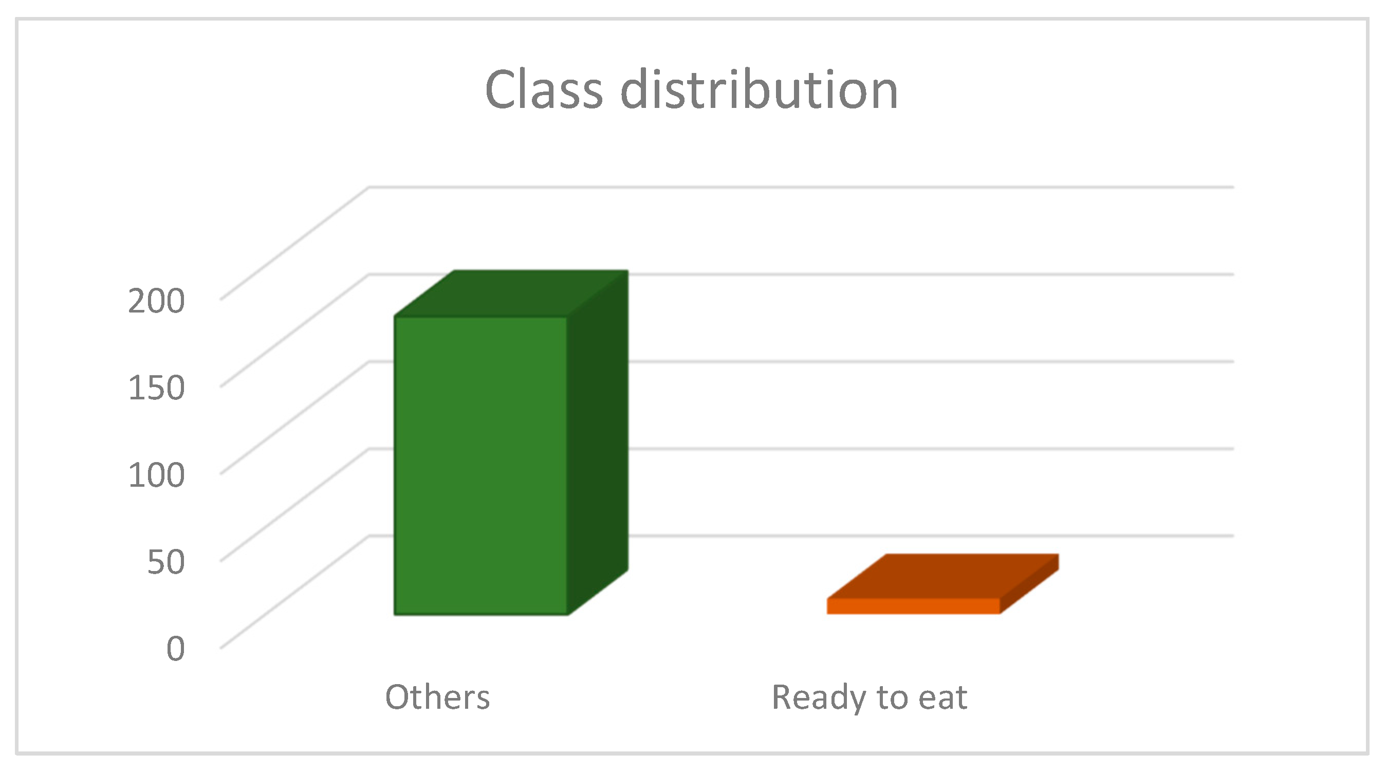
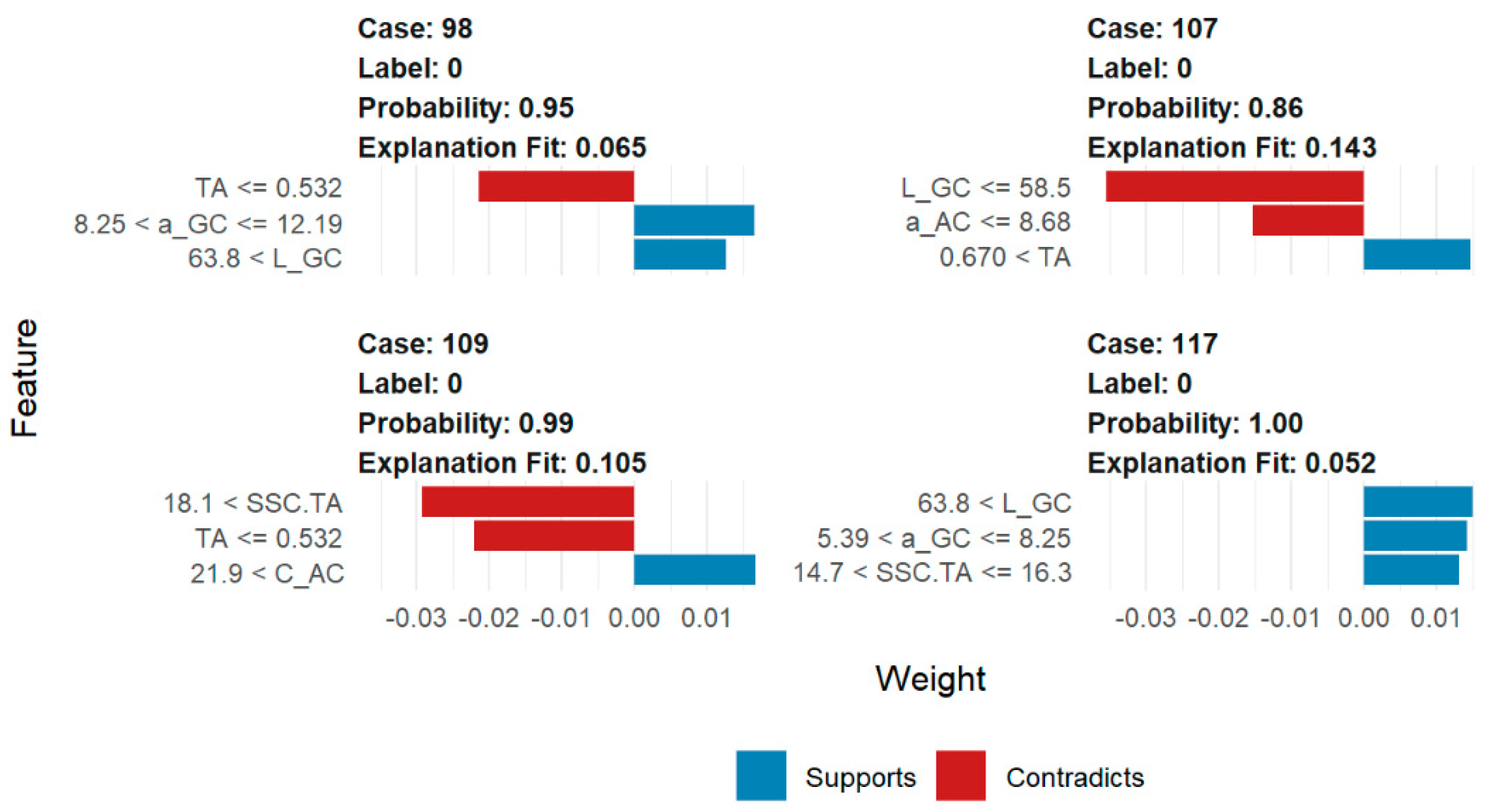
3.1. The Model A Peaches (Firmness Less Than < 1.84 kg·cm⁻²)

The Model A dataset is the most imbalanced dataset in this research, with only nine ‘ready to eat’ and 171 peaches belonging to the class ‘others’ (Figure 1).

After splitting the dataset into a training set and a test set, only two ‘ready to eat’ peaches entered the latter. An accurate model should predict only two ‘ready to eat’ peaches on a test set with another 52 peaches of the ‘others’ class. It would be very challenging to build such a model, given the size of the dataset itself. This is reflected in the results of the Random Forest model on the basic imbalanced dataset (Table 1). Although Random Forest seems to have great accuracy on the imbalanced dataset, there is not even a single ‘ready to eat’ prediction, and this can be seen from the fact that its Kappa is 0. This model predicts ‘others’ for all observations from the test set and represents a textbook example of an error on highly imbalanced datasets.

Random Forest predictions on the SMOTE balanced dataset accurately predict one out of two ‘ready to eat’ peaches from the test set, while all instances of the class ‘others’ are correctly predicted. On the other side, the ROSE model, except for one well-classified ‘ready to eat’ peach, makes many inaccurate predictions of ‘others’, and its accuracy and Kappa are significantly lower. The 95% confidence intervals (95% CIs) of 0.9011 and 0.9995 on the SMOTE balanced dataset means that there is 95% likelihood that the true accuracy for this model lies within this range. p-Value (Acc > NIR) is also the lowest in this case. Thus, the best results are obtained by applying the SMOTE method. The interpretation techniques on the SMOTE balanced Model A dataset rank variables by their importance, as shown in

Table 2. Top 10 most contributing variables in the SMOTE balanced Model A dataset.

Variable Importance		Permutation Feature Importance
TA	18.3138	L*—GC	0.076420
L*—GC	17.1416	SSC/TA	0.058790
SSC/TA	16.8870	TA	0.057410
a*—GC	12.1816	a*—GC	0.048530
a*—AC	12.0051	h°—GC	0.037430
a*/b*—GC	11.5375	CIRG1—GC	0.036020
CIRG1—GC	11.3332	COL—GC	0.032580
CCI—GC	11.1145	a*/b*—GC	0.031630
COL—GC	10.6117	CCI—GC	0.031470
h°—AC	10.2312	a*—AC	0.028260

. The most important variables in the Model A SMOTE balanced dataset are L*—GC, TA, SSC/TA, and a*—GC. These variables also prevail in the predictions of the LIME method, as evident in Figure 2.

Using the LIME algorithm to explain classifier predictions by a local approximation is a good way to validate the global interpretation method results. Case 17 in Figure 2 is a good example in which variables L_GC, a_GC, and SSC.TA determine the outcome of the prediction (probability: 1.0) and are at the very top of the most important features in the global interpretation methods used.

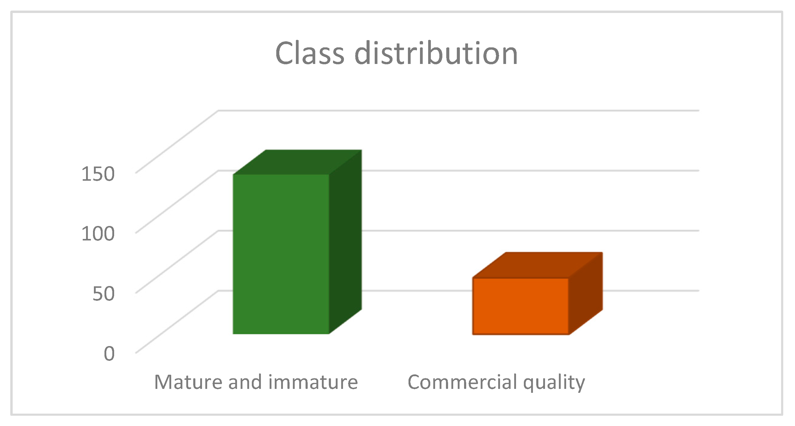
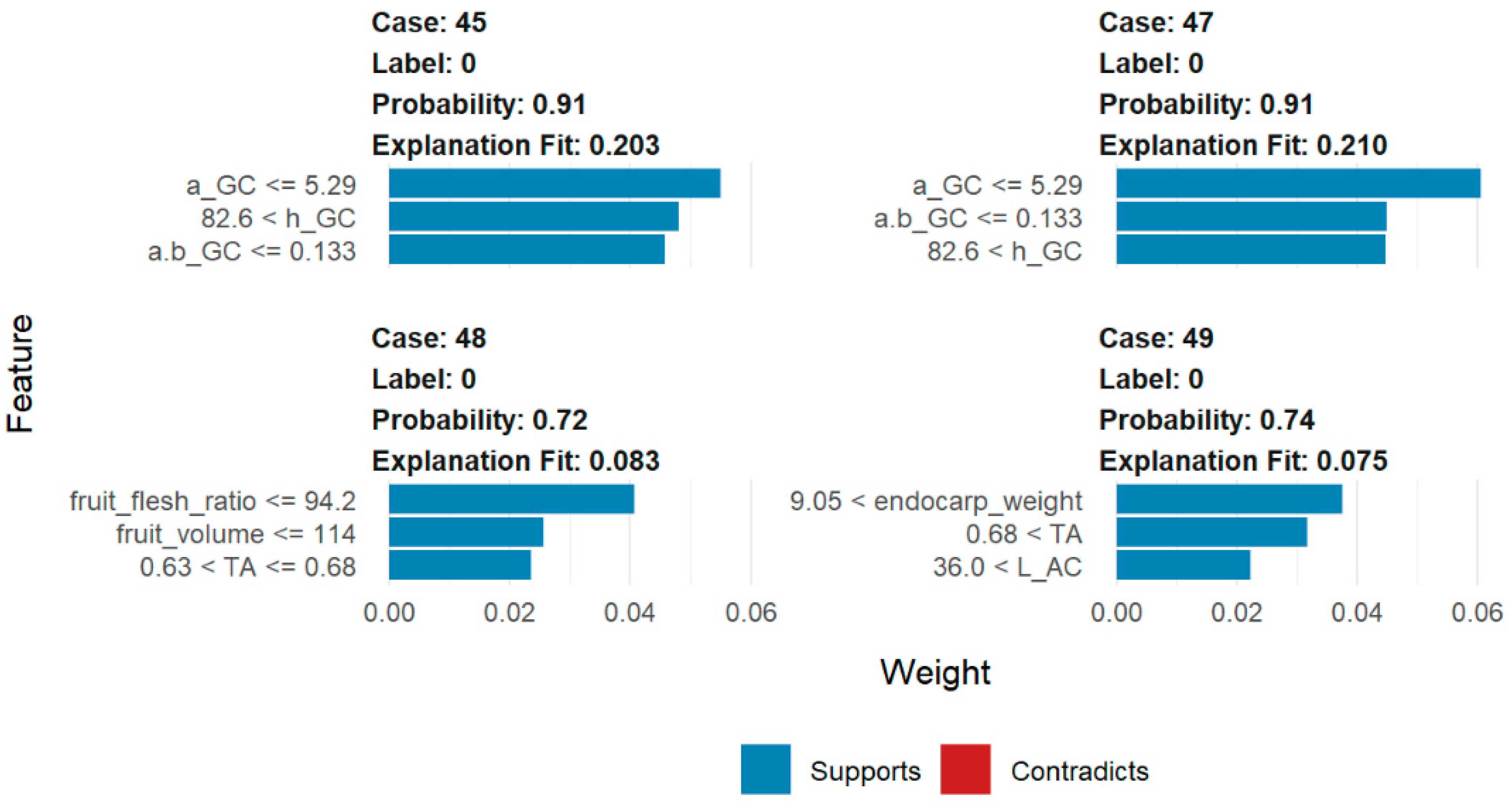
3.2. The Model B Peaches (Firmness Less Than 3.57 kg·cm⁻²)

This dataset is also imbalanced with 47 ‘commercial quality’ and 133 ‘mature and immature’ peaches (Figure 3). After applying the SMOTE and ROSE techniques to balance the datasets, the Random Forest algorithm is again used to predict peach maturity based on 33 features.

Table 3 shows that the accuracy for the ROSE balanced dataset is even worse than for the original dataset, while the accuracy for the SMOTE balanced dataset is the same as for the original dataset (81.5%).

The ratio of minority and majority class in this dataset is 35:65, and the Random Forrest algorithm makes a fairly accurate prediction of it, which is partly due to the fact that the dataset is not severely imbalanced. Therefore, predictions on the balanced datasets do not yield much higher accuracy. Moreover, in the case of predictions on the ROSE balanced dataset, the accuracy is even lower. Predictions on the SMOTE balanced dataset result with the Kappa value improved by more than 27%, which is significant. Although the SMOTE balanced dataset model has the same number of correct predictions in the same confidence interval as the original dataset model, a better distribution of false predictions (false positives and false negatives) gives it greater reliability with a better Kappa value. As already emphasized in the Section 3, the model accuracy itself is not the most reliable parameter. Therefore, the Kappa value is also used to select the best model.

Since its Kappa of 0.56 is better and therefore gives more reliable predictions and more confidence in the model, the SMOTE balanced dataset is used in the next step of interpreting variable importance.

Model interpretation methods performed on the SMOTE balanced dataset give the results shown in

Table 4. Top 10 most contributing variables in the SMOTE balanced Model B dataset.

Variable Importance		Permutation Feature Importance
a*—GC	11.476141	a*—GC	0.0395
fruit flesh ratio	10.786159	fruit flesh ratio	0.0351
endocarp weight	10.418169	h°—GC	0.0302
a*/b*—GC	9.482998	endocarp weight	0.0291
h°—GC	8.188623	a*/b*—GC	0.0273
CCI—GC	7.494602	COL—GC	0.0218
CIRG1—GC	7.446273	CCI—GC	0.0196
SSC/TA	7.318091	SSC/TA	0.0155
COL—GC	7.209811	TA	0.0134
h°—AC	5.78866	CIRG1—GC	0.0114

. Again, a very similar order of variables is determined by the two global explaining methods. The very top of both tables is occupied by a*—GC and fruit flesh ratio variables, which are, in addition to endocarp weight, the most often used variables in several random example predictions of LIME (Figure 4).

In case 47 (Figure 4), variables describing ground color features, i.e., a_GC, a.b_GC, and h_GC, determine the outcome of the prediction (probability: 0.91), and they are in the top five of the most important features in the global interpretation methods used.

3.3. The Model C Peaches (Firmness Less Than 4.59 kg·cm⁻²)

The Model C dataset is the most balanced in this study. The majority class is represented by 101 ‘appropriate’ peaches, while there are 79 ‘inappropriate’ peaches (Figure 5). The dataset is balanced by the SMOTE and ROSE algorithms so that the ratio of ripe and unripe peaches in these balanced datasets is approximately 1.

Again, the Random Forest algorithm with 10-fold cross-validation repeated three times is used, and the results are shown in Table 5.

The predictions on the ROSE balanced dataset prove to be the most accurate (77.8%) and better than the predictions on the original dataset (70.4%). The Kappa value of 0.561 on the ROSE balanced dataset shows that this model fit is noticeably better than the model fit with the original dataset and its Kappa value of 0.379. Therefore, the interpretability algorithms are performed on the ROSE balanced dataset.

The global methods for explaining the black box algorithms, i.e., Variable Importance and Permutation Feature Importance, show similar results in selecting the most important variables on the ROSE balanced dataset. COL—GC, h°—GC, fruit flesh ratio, and CCI—GC variables are among the top five most contributing variables with both algorithms (

Table 6. Top 10 most contributing variables in the ROSE balanced Model C dataset.

Variable Importance		Permutation Feature Importance
COL—GC	6.5321168	COL—GC	0.0188
h°—GC	6.0635186	h°—GC	0.0144
SSC	5.9438302	fruit flesh ratio	0.0128
CCI—GC	5.5208861	CCI—GC	0.0080
fruit flesh ratio	5.3963784	SSC/TA	0.0066
TA	4.2983678	TA	0.0062
a*—GC	3.6590949	a*—GC	0.0061
L*—AC	3.6097366	SSC	0.0057
SSC/TA	3.0672675	CCI—AC	0.0055
CIRG2—AC	2.8661167	L*—AC	0.0053

). The same variables are the most important variables in determining peach maturity in several randomly selected LIME examples (Figure 6), which confirms the results obtained previously.

Variable SSC.TA in case 88 contradicts a positive decision of the model, while the same variable supports it in case 91. In both cases, that variable is important for the prediction-making process of the Random Forest model.

4. Discussion

Based on all three model analyses, ground color parameters and indexes are evidently among the most contributing variables. The most contributing ground color parameters in all three models are h° and a*, as well as indexes COL and CCL (

Table 7. Summarization of variables that are among top 10 most contributing in all three ROSE balanced models (Models A, B, and C).

Variable Importance	Permutation Feature Importance
a*—GC (4)	h°—GC (3.33)
CCI—GC (6)	a*—GC (4)
COL—GC (6.33)	COL—GC (4.66)
SSC/TA (6.66)	SSC/TA (5)
	TA (6)

). The L* variable is the most contributing in Model A, but it is not among top ten in Model B or Model C. Similarly, index a*/b* and CIRG¹ are among the top ten contributing variables in Model A and Model B but not in Model C. However, this is not the case for additional color parameters and indexes, which contribute remarkably less and thus are not listed as in the top ten in either of the three models (Table 7). The most contributing additional color parameters are a*, L*, and h°, as well as indexes CCL and CIRG². Such a high importance of basic color variables and indexes for predicting peach maturity at harvest has been expected. Peach skin ground color presents an important maturity prediction tool [14,52,53], since it changes along with other important parameters, such as soluble solids, flesh firmness, and volatile compounds [12]. In most peach cultivars, assessment of fruit maturity by the skin ground color change includes transformation from green to yellow color [54]. Since negative a* parameter values show intensity of green color, and h° at 90 and 180° green or yellow coloration, respectively [30,31,55], the reason for their high importance in the models is obvious. Similarly, according to [56], a* and h° are good indicators of peach maturity stages since they change linearly during ripening. According to the same author, [56], these changes correlate with a decrease in chlorophyll content and an increase in the concentration of carotenoid pigments, and they reflect the changes in the activity of phenolic enzymes. However, the first (according to Permutation Feature Importance) as well as second (according to Variable Importance) most contributing color parameter in Model A is L*, which corresponds to brightness [30]. It must be noted that this dataset is very imbalanced with only nine ripe and 171 unripe peaches. This corresponds to the findings of [6], where the value of the L* parameter is most notably reduced in the last two maturity stages (out of seven total) with the increase in ripeness (decrease in firmness from 4.28 to 0.61 kg·cm⁻²). The irrelevance of the b* value in predicting peach maturity can be explained by its small changes during ripening, as indicated by [8]. Certain ground color indexes (COL, CCL, and CIRG¹) are also remarkably important for the model predictions and this highlights their potential use in peach maturity prediction. This holds especially true for the COL index, which is the most contributing feature in the Model C dataset. Regarding additional color parameters and indexes, it must be noted that their importance is considerably weaker in Variable Importance in contrast to the Permutation Feature Importance global method for explaining the black box algorithms (although it is weak in both cases). Of all the additional color parameters and indexes, according to Variable Importance, the a* parameter has the highest importance (fifth in a row) in Model A, and L* (eighth in a row) has the highest importance in Model C. This can be explained by the fact that the a* value of peach blush color generally increases during ripening, while L* decreases [57]. However, using Permutation Feature Importance, more accurate results are obtained, which shows that the usage of additional color parameter is not so reliable for maturity prediction. Peach fruit exposure to direct light is a pre-requirement for the development of red color [58]. The development of the blush color in peaches is related to the light exposure rather than to the fruit maturation [59]. The fact that peaches can be harvested from different canopy positions and orchards with or without applied nets (different light growing conditions) explains why additional color is not a reliable maturity indicator. Its low feature importance obtained in the study results confirms this rationale.

The fruit flesh ratio in Model C as well as the fruit flesh ratio and endocarp weight in Model B, are notably important variables. Peaches should be gaining weight during ripening [6,14,60,61], but fruit mesocarp and endocarp do not behave equally. The study on the Japanese plum reports that the weight curves of fruit and endocarp fresh during ripening are not related [62], which explains the importance of the fruit flesh ratio variable in the stated models. Moreover, according to the same authors [62], endocarp rapidly loses fresh weight at one moment during ripening, and afterwards, very slowly again, it starts to gain it. This might explain why endocarp fresh weight is an important parameter only in Model B.

TA and SSC/TA are important variables in all three models (Table 7), while SSC is important in Model C only. In Models B and C, TA and SSC/TA parameters are, regarding their importance (according to Variable Importance and Permutation Feature Importance), generally behind the majority of ground color parameters and indexes, as well as behind the fruit flesh ratio in Model C and fruit flesh ratio and endocarp weight in Model B. Soluble solids concentrations within certain range of titratable acidity are linked with consumer acceptance of peaches [63,64,65,66]. Therefore, they are regularly measured by producers. A general trend during peach ripening is that sugar content increases and acidity decreases [6,12,14,67,68]. Since the SSC/TA variable is related to SSC and TA parameters, its evolution during ripening is also related to them. In general, after ripening, yellow flesh peaches and nectarines lose from 10% to 30% of their TA measured at harvest; thus, their SSC/TA increases [69]. All these trends are also reported on the peach ‘Suncrest’ [60], which is the variety used in this study. SSC/TA and TA variables are among three most important variables in Model A (according to Variable Importance and Permutation Feature Importance), which is not the case with the other two models.

To a certain extent, this discussion attempts to explain why certain variables proved important in some models but not in others. Since the internal logic and work of the black box models is hidden, the users cannot fully understand the rationale behind predictions [47]. Therefore, given explanations should be taken with a word of precaution. However, it can be concluded that the importance of certain features in maturity prediction changes depending on the peach maturity stage.

The obtained results are in line with the related work presented. This adds additional confidence in the model and methods used in the study. The use of several different interpretable machine learning techniques that give very similar results further confirms the validity of the results and the usability of the model.

Although the model is created on the dataset that contains features of the peach fruit, it could be easily used on similar types of fruit for the purpose of determining the most important features in the ripening process. With some adjustments of the dataset and model parameters, it could produce just as good results as for the dataset for which it was created.

In our future work, we aim to use a much larger number of measurements that would increase the accuracy of the model and thus determine the most important maturity features. Although the Random Forest algorithm proved to be a stable and accurate machine learning model, we plan on trying out other models in order to compare prediction performances and choose the most reliable model.

5. Conclusions

In this paper, the use of interpretable machine learning techniques on the machine learning models for the purpose of discovering the most important features for peach maturity prediction proved to be justified. Expectedly, different features proved important for different maturity thresholds. The justification for such results is found to a great extent in the existing literature. In addition to the standard features used for peach maturity prediction, this study highlights the potential use of some additional features, such as COL, CCL, and CIRG¹ ground color indexes as well as fruit flesh ratio. The most prominent among them is the COL ground color index, since it proved to be the most contributing feature in Model C. Therefore, its potential should be further investigated. While the fruit flesh ratio and a*/b* ground color index are among the top ten features in two of the models, they are not among top ten in the third model. To conclude, the importance of certain features in maturity prediction changes depending on the peach maturity stage.

Although the dataset is small and at the same time extremely imbalanced, the obtained results are more than satisfactory. Even though the prediction models, due to the mentioned problems, do not always have high accuracy or reliability on the given datasets, they still manage to grasp the internal mechanisms of peach ripening prediction and obtain credible results.

References

1. Encyclopaedia Britannica Peach, Tree and Fruit. Available online: https://www.britannica.com/plant/peach (accessed on 30 June 2021).
2. Miserius, M.; Behr, D.H.-C. European Statistics Handbook; Fruitnet: London, UK, 2021; p. 3. [Google Scholar]
3. Konopacka, D.; Jesionkowska, K.; Kruczyńska, D.; Stehr, R.; Schoorl, F.; Buehler, A.; Egger, S.; Codarin, S.; Hilaire, C.; Höller, I.; et al. Apple and peach consumption habits across European countries. Appetite 2010, 55, 478–483. [Google Scholar] [CrossRef]
4. Crisosto, C.H. How do we increase peach consumption? Acta Hortic. 2002, 592, 601–605. [Google Scholar] [CrossRef]
5. Wang, X.; Matetić, M.; Zhou, H.; Zhang, X.; Jemrić, T. Postharvest quality monitoring and variance analysis of peach and nectarine cold chain with multi-sensors technology. Appl. Sci. 2017, 7, 133. [Google Scholar] [CrossRef] [Green Version]
6. Robertson, J.A.; Meredith, F.I.; Forbus, W.R. Changes in Quality Characteristics During Peach (Cv. ‘Majestic’) Maturation. J. Food Qual. 1991, 14, 197–207. [Google Scholar] [CrossRef]
7. Infante, R. Harvest maturity indicators in the stone fruit industry. Stewart Postharvest Rev. 2012, 1, 1–6. [Google Scholar] [CrossRef]
8. Shewfelt, R.L.; Myers, S.C.; Resurreccion, A.V.A. Effect of physiologycal maturity at harvest on peach quality during low temperature storage. J. Food Qual. 1987, 10, 9–20. [Google Scholar] [CrossRef]
9. Ceccarelli, A.; Farneti, B.; Frisina, C.; Allen, D.; Donati, I.; Cellini, A.; Costa, G.; Spinelli, F.; Stefanelli, D. Harvest maturity stage and cold storage length influence on flavour development in peach fruit. Agronomy 2019, 9, 10. [Google Scholar] [CrossRef] [Green Version]
10. Salunkhe, D.K.; Deshpande, P.B.; Do, J.Y. Effects of Maturity and Storage on Physical and Biochemical Changes in Peach and Apricot Fruits. J. Hortic. Sci. 1968, 43, 235–242. [Google Scholar] [CrossRef]
11. Vanoli, M.; Bianchi, G.; Rizzolo, A.; Lurie, S.; Spinelli, L.; Torricelli, A. Electronic nose pattern, sensory profile and flavor components of cold stored ‘Spring Belle’ peaches: Influence of storage temperatures and fruit maturity assessed at harvest by time-resolved reflectance spectroscopy. Acta Hortic. 2015, 1084, 687–694. [Google Scholar] [CrossRef]
12. Ramina, A.; Tonutti, P.; McGlasson, W.; McGlasson, B. Ripening, nutrition and postharvest physiology. In The Peach, Botany, Production and Uses; Layne, D.R., Bassi, D., Eds.; CAB International: Wallingford, UK, 2008; pp. 550–574. ISBN 9781845933869. [Google Scholar]
13. Crisosto, C.H.; Costa, G. Preharvest factors affecting peach quality. In The Peach: Botany, Production and Uses; CABI: Wallingford, UK, 2008; pp. 536–549. ISBN 9781845933869. [Google Scholar]
14. Shinya, P.; Contador, L.; Predieri, S.; Rubio, P.; Infante, R. Peach ripening: Segregation at harvest and postharvest flesh softening. Postharvest Biol. Technol. 2013, 86, 472–478. [Google Scholar] [CrossRef]
15. Valero, C.; Crisosto, C.H.; Slaughter, D. Relationship between nondestructive firmness measurements and commercially important ripening fruit stages for peaches, nectarines and plums. Postharvest Biol. Technol. 2007, 44, 248–253. [Google Scholar] [CrossRef] [Green Version]
16. Crisosto, C.H.; Kader, A. Peach Postharvest Quality Maintenance Guidelines; Department of Pomology, University of California: Davis, CA, USA, 2000. [Google Scholar]
17. Scalisi, A.; Pelliccia, D.; O’connell, M.G. Maturity prediction in yellow peach (Prunus persica L.) cultivars using a fluorescence spectrometer. Sensors 2020, 20, 6555. [Google Scholar] [CrossRef]
18. De-la-Torre, M.; Zatarain, O.; Avila-George, H.; Muñoz, M.; Oblitas, J.; Lozada, R.; Mejía, J.; Castro, W. Multivariate analysis and machine learning for ripeness classification of cape gooseberry fruits. Processes 2019, 7, 928. [Google Scholar] [CrossRef] [Green Version]
19. Zhang, G.; Fu, Q.; Fu, Z.; Li, X.; Matetić, M.; Bakaric, M.B.; Jemrić, T. A comprehensive peach fruit quality evaluation method for grading and consumption. Appl. Sci. 2020, 10, 1348. [Google Scholar] [CrossRef] [Green Version]
20. Hyun Cho, W.; Kyoon Kim, S.; Hwan Na, M.; Seop Na, I. Fruit Ripeness Prediction Based on DNN Feature Induction from Sparse Dataset. Comput. Mater. Contin. 2021, 69, 4003–4024. [Google Scholar] [CrossRef]
21. Varga, L.A.; Makowski, J.; Zell, A. Measuring the Ripeness of Fruit with Hyperspectral Imaging and Deep Learning. arXiv 2021, arXiv:2104.09808. [Google Scholar]
22. Ljubobratović, D.; Guoxiang, Z.; Bakarić, M.B.; Jemrić, T.; Matetić, M. Predicting peach fruit ripeness using explainable machine learning. In Proceedings of the 31st International DAAAM Virtual Symposium ‘Intelligent Manufacturing & Automation’, Mostar, Bosnia and Herzegovina, 21–24 October 2020; Katalinić, B., Ed.; DAAAM International: Vienna, Austria, 2020; pp. 717–723. [Google Scholar]
23. Taylor, R. Interpretation of the Correlation Coefficient: A Basic Review. J. Diagn. Med. Sonogr. 1990, 6, 35–39. [Google Scholar] [CrossRef]
24. Ryo, M.; Rillig, M.C. Statistically reinforced machine learning for nonlinear patterns and variable interactions. Ecosphere 2017, 8, e01976. [Google Scholar] [CrossRef]
25. Song, C.; Kwan, M.P.; Song, W.; Zhu, J. A Comparison between spatial econometric models and random forest for modeling fire occurrence. Sustainability 2017, 9, 819. [Google Scholar] [CrossRef] [Green Version]
26. Auret, L.; Aldrich, C. Interpretation of nonlinear relationships between process variables by use of random forests. Miner. Eng. 2012, 35, 27–42. [Google Scholar] [CrossRef]
27. Guidotti, R.; Monreale, A.; Ruggieri, S.; Turini, F.; Giannotti, F.; Pedreschi, D. A survey of methods for explaining black box models. ACM Comput. Surv. 2018, 51, 1–45. [Google Scholar] [CrossRef] [Green Version]
28. Krpina, I.; Vrbanek, J.; Asić, A.; Ljubičić, M.; Ivković, F.; Ćosić, T.; Štambuk, S.; Kovačević, I.; Perica, S.; Nikolac, N.; et al. Voćarstvo; Nakladni Zavod Globus: Zagreb, Croatia, 2004. [Google Scholar]
29. Miljković, I. Suvremeno Voćarstvo; Nakladni zavod Znanje: Zagreb, Croatia, 1991. [Google Scholar]
30. Hunter Associates Laboratory Inc. AN 1005.00 Measuring Color Using Hunter L, a, b Versus CIE 1976 L*a*b*. 2012, p. 4. Available online: https://www.hunterlab.com/media/documents/duplicate-of-an-1005-hunterlab-vs-cie-lab.pdf (accessed on 29 October 2021).
31. Carreño, J.; Martínez, A.; Almela, L.; Fernández-López, J.A. Proposal of an index for the objective evaluation of the colour of red table grapes. Food Res. Int. 1995, 28, 373–377. [Google Scholar] [CrossRef]
32. Gao, Y.; Liu, Y.; Kan, C.; Chen, M.; Chen, J. Changes of peel color and fruit quality in navel orange fruits under different storage methods. Sci. Hortic. 2019, 256, 108522. [Google Scholar] [CrossRef]
33. López Camelo, A.F.; Gómez, P.A. Comparison of color indexes for tomato ripening. Hortic. Bras. 2004, 22, 534–537. [Google Scholar] [CrossRef]
34. Little, A.C. A Research note: Off on a Tangent. J. Food Sci. 1975, 40, 410–411. [Google Scholar] [CrossRef]
35. Jimenez-Cuesta, M.; Cuquerella, J.; Martinez-Javaga, J.M. Determination of a color index for citrus fruit degreening. Proc. Int. Soc. Citric. 1981, 2, 750–753. [Google Scholar]
36. Hobson, G.E. Low-temperature injury and the storage of ripening tomatoes. J. Hortic. Sci. 1987, 62, 55–62. [Google Scholar] [CrossRef]
37. AOAC. AOAC Official Methods of Analysis of AOAC International, 16th ed.; 5th Rev.; Association of Official Analytical Chemists: Gaithersburg, MD, USA, 1999. [Google Scholar]
38. Crisosto, C.; Slaughter, D.; Garner, D.; Boyd, J. Stone fruit critical bruising tresholds. J. Am. Pomol. Soc. 2001, 55, 76–81. [Google Scholar]
39. Neri, F.; Brigati, S. Sensory and objective evaluation of peaches. In Proceedings of the Cost 94: The Postharvest Treatment of Fruit and Vegetables; De Jager, A., Jhonson, A., Hohn, E., Eds.; European Comission: Brussels, Belgium, 1994; pp. 107–115. [Google Scholar]
40. Viloria, A.; Lezama, O.B.P.; Mercado-Caruzo, N. Unbalanced data processing using oversampling: Machine learning. Procedia Comput. Sci. 2020, 175, 108–113. [Google Scholar] [CrossRef]
41. Douzas, G.; Bacao, F.; Last, F. Improving imbalanced learning through a heuristic oversampling method based on k-means and SMOTE. Inf. Sci. 2018, 465, 1–20. [Google Scholar] [CrossRef] [Green Version]
42. Chawla, N.V.; Bowyer, K.W.; Hall, L.O.; Kegelmeyer, W.P. SMOTE: Synthetic minority over-sampling technique. J. Artif. Intell. Res. 2002, 16, 321–357. [Google Scholar] [CrossRef]
43. Juanjuan, W.; Mantao, X.; Hui, W.; Jiwu, Z. Classification of imbalanced data by using the SMOTE algorithm and locally linear embedding. In Proceedings of the 2006 8th international Conference on Signal Processing, Guilin, China, 16–20 November 2006; Volume 3, pp. 1–4. [Google Scholar] [CrossRef]
44. Sáez, J.A.; Luengo, J.; Stefanowski, J.; Herrera, F. SMOTE-IPF: Addressing the noisy and borderline examples problem in imbalanced classification by a re-sampling method with filtering. Inf. Sci. 2015, 291, 184–203. [Google Scholar] [CrossRef]
45. Lunardon, N.; Menardi, G.; Torelli, N. ROSE: A package for binary imbalanced learning. R J. 2014, 6, 79–89. [Google Scholar] [CrossRef] [Green Version]
46. Breiman, L. Random Forests. Mach. Learn. 2001, 45, 5–32. [Google Scholar] [CrossRef] [Green Version]
47. Carvalho, D.V.; Pereira, E.M.; Cardoso, J.S. Machine learning interpretability: A survey on methods and metrics. Electronics 2019, 8, 832. [Google Scholar] [CrossRef] [Green Version]
48. Molnar, C. Interpretable Machine Learning. A Guide for Making Black Box Models Explainable. 2019, p. 247. Available online: https://christophm.github.io/interpretable-ml-book/ (accessed on 29 October 2021).
49. Vilone, G.; Longo, L. Classification of explainable artificial intelligence methods through their output formats. Mach. Learn. Knowl. Extr. 2021, 3, 615–661. [Google Scholar] [CrossRef]
50. Kuhn, M.; Johnson, K. Applied Predictive Modeling; Springer: New York, NY, USA, 2013; ISBN 978-1-4614-6849-3. [Google Scholar]
51. Ribeiro, M.T.; Singh, S.; Guestrin, C. “Why should i trust you?” Explaining the predictions of any classifier. In Proceedings of the KDD’ 16: The 22nd ACM SIGKDD International Conference on Knowledge Discovery and Data Mining, San Francisco, CA, USA, 13–17 August 2016; pp. 1135–1144. [Google Scholar] [CrossRef]
52. Infante, R.; Aros, D.; Contador, L.; Rubio, P. Does the maturity at harvest affect quality and sensory attributes of peaches and nectarines? N. Z. J. Crop Hortic. Sci. 2012, 40, 103–113. [Google Scholar] [CrossRef]
53. Crisosto, C.H.; Mitcham, E.J.; Kader, A.A. Peach and Nectarine: Recommendations for Maintaining Postharvest Quality; Postharvest Technology Center, University of California: Davis, CA, USA, 1996. [Google Scholar]
54. Crisosto, C.H.; Valero, D. Harvesting and postharvest handling of peaches for the fresh market. In The Peach: Botany, Production and Uses; Layne, D.R., Bassi, D., Eds.; CAB International: Wallingford, UK, 2008; pp. 575–596. ISBN 9781845933869. [Google Scholar]
55. Fruk, G.; Fruk, M.; Vuković, M.; Buhin, J.; Jatoi, M.A.; Jemrić, T. Colouration of apple cv. ‘Braeburn’ grown under anti-hail nets in Croatia. Acta Hortic. Regiotect. 2016, 19, 1–4. [Google Scholar] [CrossRef] [Green Version]
56. Ferrer, A.; Remón, S.; Negueruela, A.I.; Oria, R. Changes during the ripening of the very late season Spanish peach cultivar Calanda: Feasibility of using CIELAB coordinates as maturity indices. Sci. Hortic. 2005, 105, 435–446. [Google Scholar] [CrossRef]
57. Orazem, P.; Mikulic-Petkovsek, M.; Stampar, F.; Hudina, M. Changes during the last ripening stage in pomological and biochemical parameters of the “Redhaven” peach cultivar grafted on different rootstocks. Sci. Hortic. 2013, 160, 326–334. [Google Scholar] [CrossRef]
58. Westwood, M.N. Temperate-Zone Pomology: Physiology and Culture; Timber Press: Portland, OR, USA, 1993; ISBN 0881922536, ISBN 9780881922530. [Google Scholar]
59. Cecilia, M.; Nunes, N. Color Atlas of Postharvest Quality of Fruits and Vegetables; John Wiley & Sons, Inc.: Hoboken, NJ, USA, 2008; Volume 44, ISBN 9780813817521. [Google Scholar]
60. Selli, R.; Sansavini, S. Sugar, acid and pectin content in relation to ripening and quality of peach and nectarine fruits. Acta Hortic. 1995, 379, 345–358. [Google Scholar] [CrossRef]
61. Wu, B.H.; Quilot, B.; Génard, M.; Kervella, J.; Li, S.H. Changes in sugar and organic acid concentrations during fruit maturation in peaches, P. davidiana and hybrids as analyzed by principal component analysis. Sci. Hortic. 2005, 103, 429–439. [Google Scholar] [CrossRef]
62. Famiani, F.; Casulli, V.; Baldicchi, A.; Battistelli, A.; Moscatello, S.; Walker, R.P. Development and metabolism of the fruit and seed of the Japanese plum Ozark premier (Rosaceae). J. Plant Physiol. 2012, 169, 551–560. [Google Scholar] [CrossRef] [PubMed]
63. Crisosto, C.H.; Crisosto, G.M. Relationship between ripe soluble solids concentration (RSSC) and consumer acceptance of high and low acid melting flesh peach and nectarine (Prunus persica (L.) Batsch) cultivars. Postharvest Biol. Technol. 2005, 38, 239–246. [Google Scholar] [CrossRef]
64. Crisosto, C.H.; Crisosto, G. Searching for consumer satisfaction: New trends in the California peach industry. In Proceedings of the Ist Mediterranea Peach Symposium, Agrigento, Italy, 10 September 2003. [Google Scholar]
65. Crisosto, C.H.; Crisosto, G.; Bowerman, E. Understanding consumer acceptance of peach, nectarine and plum cultivars. Acta Hortic. 2003, 604, 115–119. [Google Scholar] [CrossRef]
66. Kader, A.A. Fruit maturity, ripening, and quality relationships. Acta Hortic. 1999, 485, 203–208. [Google Scholar] [CrossRef]
67. Bae, H.; Yun, S.K.; Jun, J.H.; Yoon, I.K.; Nam, E.Y.; Kwon, J.H. Assessment of organic acid and sugar composition in apricot, plumcot, plum, and peach during fruit development. J. Appl. Bot. Food Qual. 2014, 87, 24–29. [Google Scholar] [CrossRef]
68. Zheng, B.; Zhao, L.; Jiang, X.; Cherono, S.; Liu, J.J.; Ogutu, C.; Ntini, C.; Zhang, X.; Han, Y. Assessment of organic acid accumulation and its related genes in peach. Food Chem. 2021, 334, 127567. [Google Scholar] [CrossRef]
69. Crisosto, C.H.; Day, K.R.; Crisosto, G.M.; Garner, D. Quality attributes of white flesh peaches and nectarines grown under California conditions. Fruit Var. J. 2001, 55, 45–51. [Google Scholar]
Figure 1. Distribution of ‘others’ and ‘ready to eat’ classes of peaches in the Model A dataset.
Electronics 10 03115 g001
Figure 2. A few random LIME predictions on the Model A dataset. (Due to the inability to use special characters in the programming language, feature names are slightly modified, as described in Appendix A).
Electronics 10 03115 g002
Figure 3. Distribution of ‘mature and immature’ and ‘commercial quality’ classes in the Model B dataset.
Electronics 10 03115 g003
Figure 4. Four random LIME predictions on the Model B dataset. (Due to the inability to use special characters in the programming language, feature names are slightly modified, as described in Appendix A).
Electronics 10 03115 g004
Figure 5. Distribution of ‘inappropriate’ and ‘appropriate’ classes in the Model C dataset.
Electronics 10 03115 g005
Figure 6. Several random samples of the LIME method on the Model C dataset. (Due to the inability to use special characters in the programming language, feature names are slightly modified, as described in Appendix A).
Electronics 10 03115 g006