Harmonics Reduction and Reactive Power Injection in Wind Generation Systems

Abstract

In this work, methods are implemented to improve two aspects of energy quality in a wind generation system. First, the harmonic reduction is achieved by applying a linear control technique in the Grid Side Converter; and second, the power factor of the wind generation system using a Doubly Fed Induction Generator (DFIG) is adjusted by injecting reactive power. The reduction of the harmonic content is performed with a digital resonant controller, which tracks the periodic signals corresponding to the current harmonics of the Grid Side Converter (GSC), which is part of a “back to back” converter in a wind generation system. This technique allows implementing a current controller of the GSC with a high level of rejection of current harmonics, of frequencies with orders (1 + 6k) and (1 − 6k) (where k is an integer), when executed in the synchronous reference frame (dq). The purpose of this work is to inject currents to the grid with very low harmonic distortion and provide a method for tuning the resonant controller for a simple L filter; also, the GSC is used to generate reactive power. These two improvements achieve a unity power factor, and this is necessary to comply with the new codes where a leading power factor helps regulate the grid voltage.

1. Introduction

For many nations, maintaining an energy mix with a wide diversity of sources is a necessary key to achieve energy independence, which allows nations to avoid import energetics (such as fuel and electric power transmission from neighboring countries). Import energetics create risky situations when the global energy supply chain fails, which will be relevant as the demand increases again as activities resume under the “new normality” resulting from the COVID–19 global pandemic [1]. In addition, unexpected fails in transport routes [2] affect the population and local economy, causing price volatility in consumer goods and running the risk of black-outs in countries dependent on external sources. Wind energy is a solution for any country with potential for generating this type of energy. The use of electronic power converters in wind generation systems among other features allows the use of AC machines in variable speed systems [3]. Some of the most significant applications are in Permanent Magnet Synchronous Generators (PMSGs), whose scheme uses an electronic converter to perform the power and speed control, as well as to interconnect to the grid, operating at variable power and speed instead of working synchronized to the grid [3]. Another example is the Doubly Fed Induction Generator (DFIG) that is studied in this work, where the stator is directly connected to the grid, and the control is done with a “back to back” converter connected to the rotor and the grid. This scheme takes advantage of the wide slip range of the machine, which most manufacturers design to be around 30% above the synchronous speed (hypersynchronous operation) and 30% below the synchronous speed (subsynchronous operation) [4]. The back-to back converter allows the implementation of a vector control scheme to control the speed and generated power of the machine using the rotor voltages and currents. These particular characteristics are applied when it is required to inject power through the rotor during subsynchonous operation or to generate power through the rotor during hypersynchronous operation, where the maximum injected or extracted power is commonly 30% of the rated power [4]. The electronic converters used in these kinds of schemes often suffer from harmonic distortion, impacting the overall THD of the wind generation system, with harmonic components injected to the grid by the Grid Side Converter (GSC). Recent standards and codes implemented in different countries are aimed at renewable energy sources, demanding they operate with high power quality. Some codes regulate the harmonic content and establish a maximum THD on voltages and currents delivered by these sources. One of these is the standard IEEE 519–2014 [5] and its section for renewable energy sources. In addition, a standard for distributed systems IEEE 1547–2018 [6] outlines a maximum permissible distortion and harmonic levels. Additionally, standards such as the IEC 61000–4–30 define methods to perform measurements of the power quality [7]. 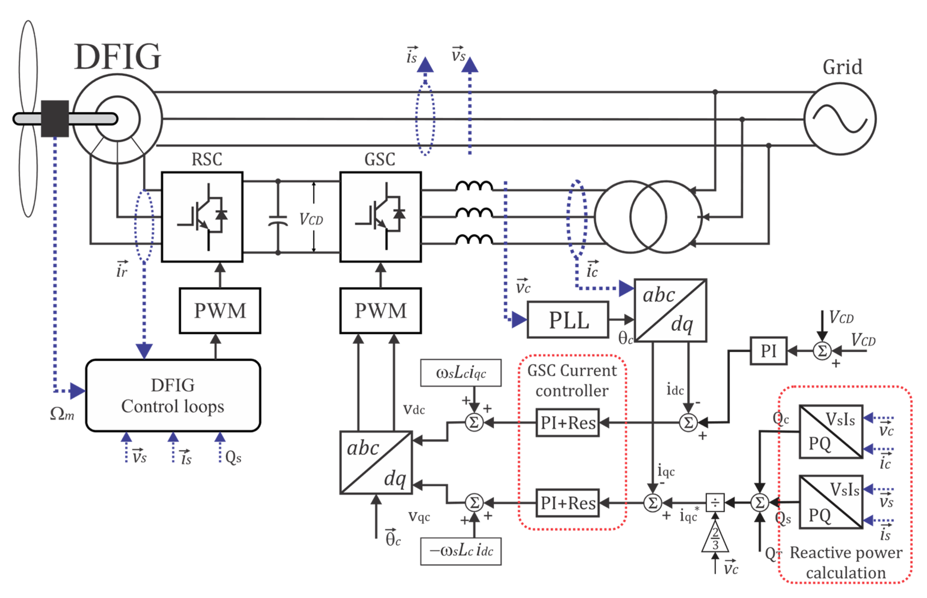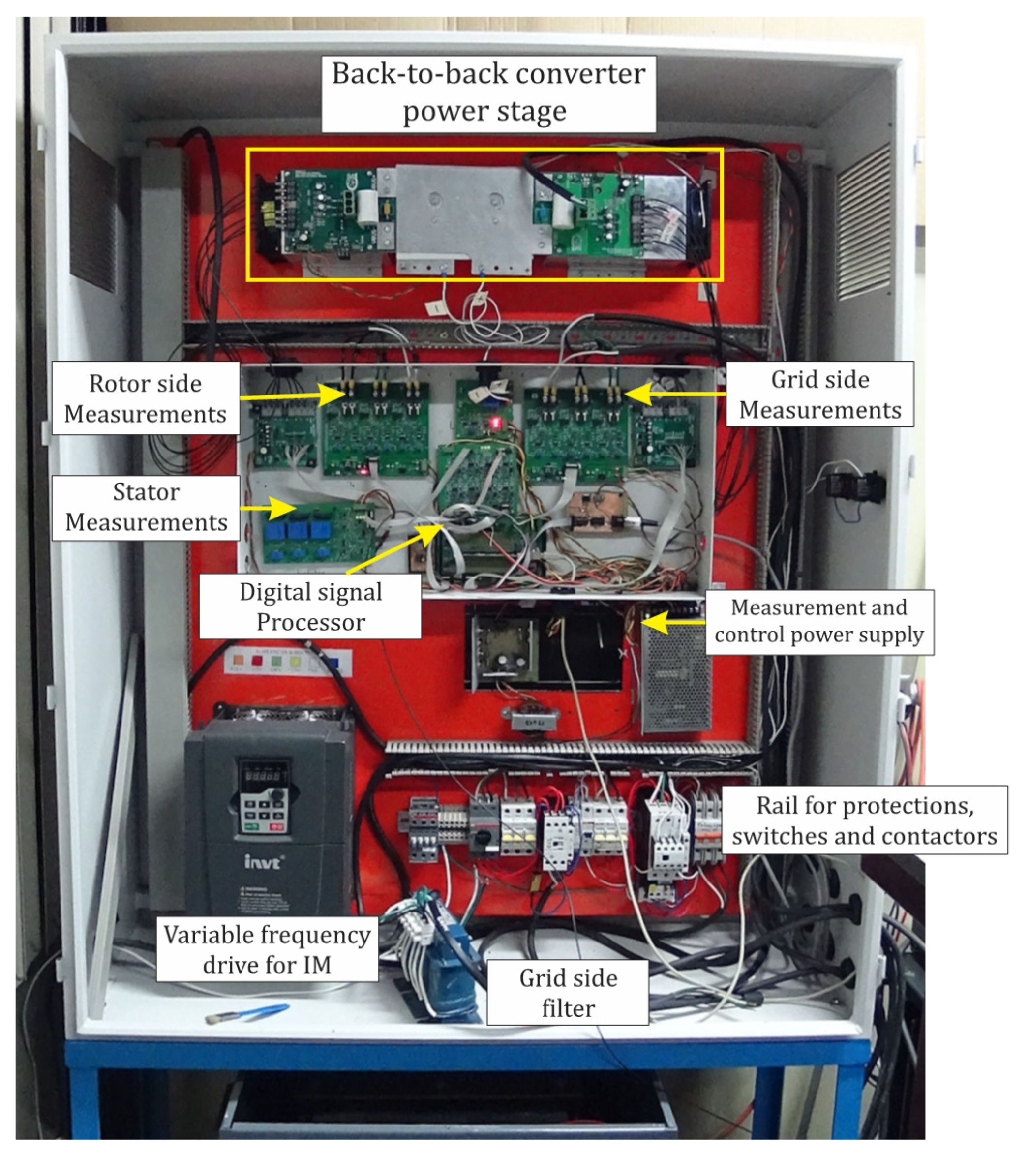Another trend in Wind Generation Systems (WGS) used in distributed generation is the ability to regulate the grid voltage by injecting reactive power to the grid [8]. The GSC is part of a “back to back” converter in the WGS, and it is shown by Figure 1. This system uses a Doubly Fed Induction Generator (DFIG), where the converter is designed with a proposed maximum active power (rated) 30% of the rated power of the DFIG [3,4].

The semiconductors used in power electronic converters such as Insulated Gate Bipolar Transistor (IGBT) require the introduction of a dead time to avoid shoot-through currents to the DC link caused by the turn off time of these semiconductors [9]. The dead time introduces distortion to the output voltages and currents, manifesting as crossover distortion and trimming on the peaks and valleys of the sinusoidal current [10].

In addition, there is an interaction of the converters with voltage harmonics present in the grid voltages [11]. Vector control schemes implementing conventional Proportional Integral controllers (PI) are unable to mitigate the distortion on the converter currents [12]. This is due to the classical PI type controllers used in vector control schemes having a poor performance when tracking time-varying signals [13]. In [14], PI+Resonant controllers were presented in the synchronous reference frame (dq) implementing ideal resonant functions, which are difficult to implement in economic Digital Signal Processor-based controllers, whose limited bit resolution may cause numerical errors, which can lead to numerical instability or deviation in the tracking frequency of the controller. Additionally, a variation on the grid frequency with respect to the tracking frequency may result in an abrupt decrease in the ability to track and compensate the harmonics on the inverter currents [15].

The need for tracking and compensating current harmonics, which are time-varying signals, discard many techniques from classical control. Among the options that have been proposed to solve this problem, there are some based on nonlinear control techniques, such as those based on sliding mode control (SMC), predictive control, and hysteresis band current controllers, among others [16,17,18]. In addition, some control schemes using Proportional+Resonant (PR) controllers in the stationary (αβ) were proposed [15], where the fundamental frequency is also tracked with a resonant controller. In the case of implementation with SMC, THD levels lower than 5% can be achieved; however, the implementations carried out show that this control presents a high frequency ripple, which is usually above 2 kHz, which is caused by the sliding nature of this type of controller when tracking a reference [19]. This oscillation is often referred to as “chattering” [18]. More advanced schemes of SMC (second order sliding modes, such as “supertwisting”) manage to mitigate this effect without it disappearing completely. Additionally, the mathematical complexity of SMC increases, which makes tuning this type of controllers difficult. Control techniques such as hysteresis band and predictive observers [20,21] are characterized by strong electromagnetic emissions due to the high amplitude current ripple required by these techniques to ensure its convergence. Other control algorithms based on nonlinear control techniques often involve the use of transcendental functions in its calculations [16,17,19], creating a greater processing load to the DSP with the numerical approximations required by these transcendental functions, and executed through a variable number of clock cycles.

Additionally, a reactive power control loop was added to this scheme, allowing the GSC to generate and inject reactive power to the grid; this controller is used in conjunction with the reactive power control of the GIDA, which is implemented in the machine control loops to control the total reactive power of the wind generation system [22]. Such implementation allows the operator of the power grid to regulate and stabilize the voltage of the grid using the reactive power from the turbine, commanding the wind turbine to inject reactive power into the grid when the voltage is below its rated value or consume reactive power when the grid voltage is above its rated value. In other words, through a variation from a lagging power factor to a leading power factor, the system fulfills simultaneously the power generation function as well as the functions of a Synchronous Static Compensator (STATCOM) [8].

In this work, a non-ideal resonant controller with a defined bandwidth is used to compensate for deviations in the line frequency when placed in parallel to the Proportional–Integral (PI) current controller of the GSC on the synchronous reference frame (dq). The resonant controller tracks the harmonic frequencies, while the PI controller tracks the reference corresponding to the fundamental of current and controls the voltage of the DC link in the back-to-back converter. In [14], besides of the use of ideal resonant controllers, a method for tuning these controllers is absent, and in [15], the convergence of the tuning method relies on the extra poles from an LCL filter, considering a PR controller with its respective degrees of freedom. The presented work shows a method for tuning the PI+Resonant controller considering a simple L filter and the delays introduced by the converter and discretization from the A/D converters. The implementation was carried out in a Digital Signal Processor (DSP), where the digital resonant controllers are implemented in the form of an Infinite Impulse Response (IIR), which is characterized by consuming very little processing time and resources from the DSP requiring simple arithmetic operations by the algorithm. This is because the DSP architecture was conceived to perform this type of operations efficiently, using instruction segmentation known as “pipeline” [23], allowing it to execute the calculations of multiple discrete transfer functions, and using a small and fixed number of clock cycles as well as single cycle instructions.

2. Grid-Side Converter Model

The back to back converter is shown in Figure 1; it is composed of two three-phase converters with six switches connected by a DC link. The present work focuses on the GSC; therefore, the analyzed model corresponds to this converter, which is connected to the grid through an L filter. The GSC operates as a voltage source, where the filter voltage drop is equal to the voltage difference between the converter and grid. By knowing the filter model, it is possible to control the current between the GSC and the grid, allowing the transfer of active power or generating reactive power between the converter and the grid. To implement the GSC control structure, it is necessary to find the converter dynamic model, which is determined by [24]:

$$\begin{array}{c}{v}_{Ca}\left(t\right)=r_l{i}_{Ca}\left(t\right)+L\frac{{di}_{Ca}\left(t\right)}{dt}+v_{Sa}\left(t\right)\\ v_{Cb}\left(t\right)=r_l{i}_{Cb}\left(t\right)+L\frac{{di}_{Cb}\left(t\right)}{dt}+v_{Sb}\left(t\right)\\ v_{Cc}\left(t\right)=r_l{i}_{Cc}\left(t\right)+L\frac{{di}_{Cc}\left(t\right)}{dt}+v_{Sc}\left(t\right)\end{array},$$

(1)

where v_Ca, v_Cb, and v_Cc are the voltages at the three-phase output of the GSC, r_l and L are the resistance and inductance of the filter, respectively, i_Ca, i_Cb, and i_Cc are the GSC currents, and v_Sa, v_Sb, and v_Sc are the voltages in the transformer secondary, which are expressed by:

$${\overrightarrow{v}}_s^s(t)=\frac{2}{3}(V_{Sa}{a}^0+V_{Sb}a+V_{Sc}{a}^2)e^{j{\omega }_{s}t},$$

(2)

where ${a=e}^{j2\pi /3}$ and $V_{Sa}{,V}_{Sb}{,V}_{Sc}$ are the peak values on the transformer secondary voltage, and ω_s is the angular frequency of the grid. A vector control scheme is used, which requires a model of the converter in the synchronous reference frame (dq) [25]. To do this, a transformation of the equations system (1) from a three-phase reference frame to a synchronous reference frame is done, using the Park transform expressed by (3).

$${\overrightarrow{x}}^a=\left[\begin{array}{c}{x}_d\\ xq\end{array}\right]=\frac{2}{3}\left[\begin{array}{ccc}cos\theta & cos(\theta -\frac{2}{3}\pi )& (\theta -\frac{2}{3}\pi )\\ sin\theta & sin(\theta -\frac{2}{3}\pi )& sin(\theta -\frac{2}{3}\pi )\end{array}\right]\left[\begin{array}{c}{x}_a\\ x_b\\ x_c\end{array}\right],$$

(3)

Considering that the synchronous reference frame (dq) rotates at the same angular speed as the voltage vector, the voltage vector is oriented with the d axis, so that the projection of the voltage vector is $v_{sd}=\left|{\overrightarrow{v}}_s\right|$ y $v_{sq}=0$. With these considerations, the dynamic model of the converter in the synchronous reference frame is expressed by:

$$\begin{array}{c}{v}_{Cd}(t)=r_l{i}_{Cd}(t)+L\frac{d{i}_d(t)}{dt}-{\omega }_{s}L{i}_{Cq}(t)+\left|{\overrightarrow{v}}_s\right|\\ v_{Cq}(t)=r_l{i}_{Cq}(t)+L\frac{d{i}_q(t)}{dt}+{\omega }_{s}L{i}_{Cd}(t)\end{array},$$

(4)

where v_Cd, v_Cq, i_d, and i_q, are the converter voltages and currents in the synchronous reference frame, respectively. The terms e_q and e_d are introduced to the system to perform the decoupling of the coordinate axes.

$$\begin{array}{c}{e}_q{=-\omega }_s{Li}_{Cq}\left(t\right)\\ e_d{=\omega }_s{Li}_{Cd}\left(t\right)\end{array},$$

(5)

The implementation of a decoupling structure is shown in Figure 1, where the terms (5) introduced on the current loop this structure are known as “Feedforward” [12]. Adding (5) to (4) the decoupled equation system gives:

$$\begin{array}{c}{v}_{Cd}(t)=r_l{i}_{Cd}(t)+L\frac{d{i}_{cd}(t)}{dt}+\left|{\overrightarrow{v}}_s\right|\\ v_{Cq}(t)=r_l{i}_{Cq}(t)+L\frac{d{i}_{cq}(t)}{dt}\end{array}.$$

(6)

Applying the Laplace transform to each of the decoupled parts of Equation (6), the resulting transfer functions of the converter currents are expressed in (7) and (8). The transfer functions include a time delay T_d, which is introduced by the conversion time of the A/D converters of the digital signal processor (DSP) as well as the delay introduced by the converter by the PWM modulation. The inclusion of this delay is necessary to guarantee convergence on the calculations in the design procedure of the resonant gains of the controller.

$$G_{id}\left(s\right)=\frac{i_d\left(s\right)}{v_{Cd}\left(s\right)}=\frac{1}{r_L+sL}{e}^{-s{T}_d},$$

(7)

$$G_{iq}\left(s\right)=\frac{i_q\left(s\right)}{v_{Cq}\left(s\right)}=\frac{1}{r_L+sL}{e}^{-{sT}_d},$$

(8)

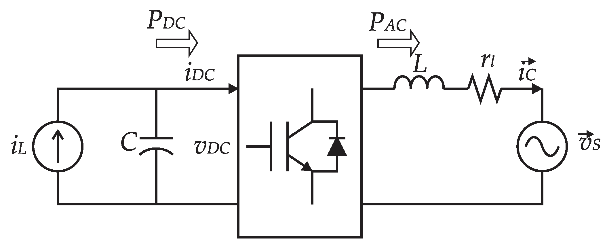
To model the DC link external loop, a relation between the DC side and the grid side is established, according to Figure 2, where said power can be approximately the same, when the converter losses are neglected. Previous works use only the capacitor model to establish the DC bus transfer function [12]. However, a transfer function can also be established around the permanent regime set point to obtain a better rejection of perturbations from the load.

The DC bus voltage equation is obtained approximating between the instantaneous power of the DC bus and the grid active power.

$$P_{AC}{=P}_{DC}{=v}_{DC} i_L\left(t\right)-v_{DC}C\frac{{dv}_{DC}\left(t\right)}{dt}{=v}_{Sd} i_{cd}{+v}_{Sq} i_{cq}$$

(9)

Considering that a control oriented in the d axis is implemented, the terms in the orthogonal axis q are equal to zero; with this consideration, a small signal analysis is done in (9) to obtain:

$$V_{DC}{\hat{i}}_L+{\hat{v}}_{DC}{I}_L-V_{DC}C\frac{d{\hat{v}}_{DC}}{dt}=V_{Sd}{\hat{i}}_{Cd}+{\hat{v}}_{Sd}{I}_{Cd}$$

(10)

where the set point on the permanent regime is given by the nominal bus voltage V_DC and the inverter nominal current I_L of the DC link, V_Sd is the line voltage, and I_Cd is the nominal current on the d axis. In (10), these set point variables are considered constants; for the small signal variables, the output current variation ${\hat{i}}_L$ and the grid voltage variation ${\hat{v}}_d$ are considered disturbances. The small signal component of the bus voltage ${\hat{v}}_{DC}$ and the grid-side current ${\hat{i}}_d$ are the output and input respectively, applying the Laplace transform to (10). The resulting transfer function is:

$$G_{VDC}(s)=\frac{{\hat{v}}_{DC}\left(s\right)}{{\hat{i}}_{Cd}(s)}=\frac{-V_{Sd}}{s{V}_{DC}C-I_L},$$

(11)

3. Harmonic Analysis in the dq Synchronous Reference Frame

The current harmonics in three-phase converters are due to the insertion of dead times in the semiconductors, switching signals to avoid shoot-through currents in the legs of the converter, also from the interaction of the converter with voltage harmonics. The introduction of dead times produces symmetric distortion that is observed as interruptions in the waveform of the inverter currents on the grid side; this is reflected in odd harmonics appearing, whose frequencies are adjacent to multiples of 6, that is (1 + 6k) (where k is a positive integer), which are positive sequence harmonics, and negative sequence harmonics with frequencies on orders of (1 − 6k) [10]. In the harmonics caused by the distortion in the grid voltage, the most common type of distortion is symmetric; therefore, odd harmonics are also present [11]. For its analysis, harmonic functions are shown in its Euler form.

$${\overrightarrow{h}}_{1+6k}^s(t)+{\overrightarrow{h}}_{1-6k}^s(t)A_{1+6k}{e}^{j{\omega }_s(1+6k)t}+A_{1-6k}{e}^{j{\omega }_s(1-6k)t}$$

(12)

Expressing the Park transformation as the operator $e^{-j{\omega }_s}$, and applying it to the harmonic vectors to obtain equivalent vectors in the synchronous reference frame:

$${\overrightarrow{h}}_{1+6k}^s(t)e^{-j{\omega }_s}+{\overrightarrow{h}}_{1-6k}^s(t)e^{-j{\omega }_s}=A_{1+6k}{e}^{j6k{\omega }_{s}t}+A_{1-6k}{e}^{j6k{\omega }_{s}t}.$$

(13)

In the current loop, the resulting functions are the product of the addition of each pair of frequencies when shifted as a result of the transformation and are expressed by the functions:

$${\overrightarrow{h}}_{6k}^a=\left[\begin{array}{c}(A_{1+6k}+A_{1-6k})cos6k{\omega }_{s}t\\ (A_{1+6k}+A_{1-6k})sen6k{\omega }_{s}t\end{array}\right].$$

(14)

From this analysis, it is observed that the adjacent of harmonics (1 + 6k) and (6k − 1) shift their frequencies to 6k and their amplitudes are added. When the current control is realized in the synchronous reference frame (dq), the vector components of the current fundamental appear as continuous signals in the (dq) axes, and the ripple on these signals corresponds to the current harmonics (14).

4. Reactive Power Control of the Grid-Side Converter

Current codes on wind generation systems require these systems to operate with a near unity power factor (fp), considering both reactive power and harmonic content [6]. In other cases, it is required for the system to be able to control the reactive power, meaning that the system can either consume reactive power obtaining a lagging fp = 0.9, or to inject reactive power to the grid, achieving a leading power factor to help regulate the grid voltage [8]. A structure for controlling the GSC reactive power is added to the control loops of the converter, which is used to generate the current reference $Q_c^{*}$ based on the balance of reactive power consumed by the stator of the DFIG Q_s and the required total reactive power Q_T.

$$Q_c^{*}{=Q}_s-Q_T$$

(15)

From the PQ theory [25], the power relations in the synchronous reference frame (dq) are described by:

$$\begin{array}{c}{P}_c=\frac{3}{2}\left(v_{sd}{i}_{cd}{+v}_{sq}{i}_{cq}\right)\\ Q_c=\frac{3}{2}\left(v_{sq} i_{cd}-v_{sd} i_{cq}\right)\end{array}.$$

(16)

To obtain the current references in an oriented control scheme, the consideration ($v_{sd}=\left|{\overrightarrow{v}}_s\right|$ and $v_{sq}=0$) is used. The power Equation (16) for the reactive power becomes $Q_c=3/2\left(v_{sd} i_{cq}\right)$, which depends only on the q component of the current. Taking this into account the current reference $i_{cq}^{*}$ is:

$$i_{cq}^{*}=\frac{2}{3}\frac{Q_c}{v_{sd}}.$$

(17)

5. PI+Resonant Current Controller

The proposed PI+Resonant controller is implemented in the synchronous reference frame, unlike [26], where a similar scheme is realized in the stationary reference frame αβ. In the proposed implementation, the PI part of the controller is responsible for monitoring the fundamental currents and controlling of the voltage on the DC bus, while the resonant controllers track the equivalent harmonic components of the reference currents $i_d^{*}$ and $i_q^{*}$. A typical resonant controller has the form shown in (18) [27].

$$H_{k,n}\left(s\right)=\frac{K_{Rn}{\omega }_{n}s}{s^2{+\omega }_n^2}$$

(18)

The controller in (18) is an ideal form of this type of controller; however, as shown in [28], the implementation of this controller is not suitable in digital systems because of the limited numerical precision these systems have; for this reason, the proposed controllers have the form:

$$H_{k,n}\left(s\right)=\frac{K_{Rn}{2\xi n\omega }_{s}s}{s^2+{2\xi n\omega }_{s}s+{n\omega }_s^2}.$$

(19)

This form allows its practical implementation and introduces a damping factor ξ in this controller to provide stability against the numerical instability caused by the numerical resolution; also, the added bandwidth is useful: when a shift occurs on the grid frequency, the controller will maintain tracking. The proposed transfer function of the PI+Resonant controller for both axes is:

$$H_i\left(s\right)=K_p+\frac{K_i}{s}+{{\displaystyle \sum }}_{n=6k}^{24} \frac{K_{Rn}{2\xi n\omega }_{s}s}{s^2+{2\xi n\omega }_{s}s+{\left(n{\omega }_s\right)}^2},$$

(20)

where ω_s is the grid frequency, multiplied by the index n to designate the equivalent harmonic in the synchronous reference frame, ξ is the damping factor of the resonant controller, and K_Rn.

5.1. PI Controller Tuning for Current and Voltage Control Loops

Considering that each resonant controller tracks two harmonic frequencies, according to the analysis in Section 2, the PI controller should work on the fundamental component of the current, with a constant reference on the synchronous reference frame dq. In [12], the design of the controller is done considering a fixed overshoot and making crossover frequency ω_c the inverse of the time constant of the plant. The calculations in the cited work were obtained from the Bode plot, where ω_c is the point where the open-loop transfer function gain (21) is unitary (0 dB).

$$G_{olidq}\left(s\right){=H}_i\left(s\right)G_i\left(s\right)$$

(21)

A variation to this method is to consider a different crossover frequency ω_c and a phase margin (PM) according to the desired overshoot level [29]. Equation (22) corresponds to the point with unity gain, while (23) corresponds to the phase margin at that point.

$$\Vert H_i\left(s\right)G_i\left(s\right)\Vert {}_{s=j{\omega }_{ic}}=1,$$

(22)

$$\measuredangle {H_i\left(s\right)G_i\left(s\right)|}_{{s=j\omega }_{ic}}{=PM}_{ic}-180°$$

(23)

Substituting the current loop transfer functions (8) and the PI part of the controller (17) in (22) and (23), they form a system of equations which is solved for K_p and K_i obtaining (24) and (25).

$$K_p=\frac{r_L{+LMFk\omega }_{ic}}{\sqrt{{MFk}^2+1}},$$

(24)

$$K_i=\frac{{L\omega }_{ic}^2{-r}_L{MFk\omega }_{ic}}{\sqrt{{MFk}^2+1}},$$

(25)

where ${MFk}_{ic}=tan\left({PM}_{ic}-\pi \right)$. The values of ω_ic and PM_ic are proposed considering the desired speed response of the control loop, where the current loop is designed with a crossover frequency one decade below the switching frequency ω_sw and above the fundamental frequency of the grid ω_s, ω_s < ω_ic < 0.1ω_sw. The gains of the voltage loop controller are obtained starting from the closed-loop current transfer function:

$$G_{clidq}\left(s\right)=\frac{i_{dq}\left(s\right)}{v_{dq}\left(s\right)}=\frac{G_{olidq}\left(s\right)}{{1+G}_{olidq}\left(s\right)}.$$

(26)

A crossover frequency ω_VCDc is chosen to be at least one decade below the crossover frequency of the current loop, ω_VCDc < 0.1ω_ic, and a proposed phase margin PM_VCD, which is usually of π/3 depending on the desired transient response. The resulting equations are

$$K_{Pdc}=\frac{I_L{+CMFk}_{cd}{V}_{DC}{\omega }_{cd}}{V_{Sd}\sqrt{{MFk}_{\Omega }^2+1}},$$

(27)

$$K_{Idc}=\frac{I_L{MFk}_{cd}{\omega }_{cd}-{CV}_{CD}{\omega }_{cd}^2}{V_{Sd}\sqrt{{MFk}_{\Omega }^2+1}},$$

(28)

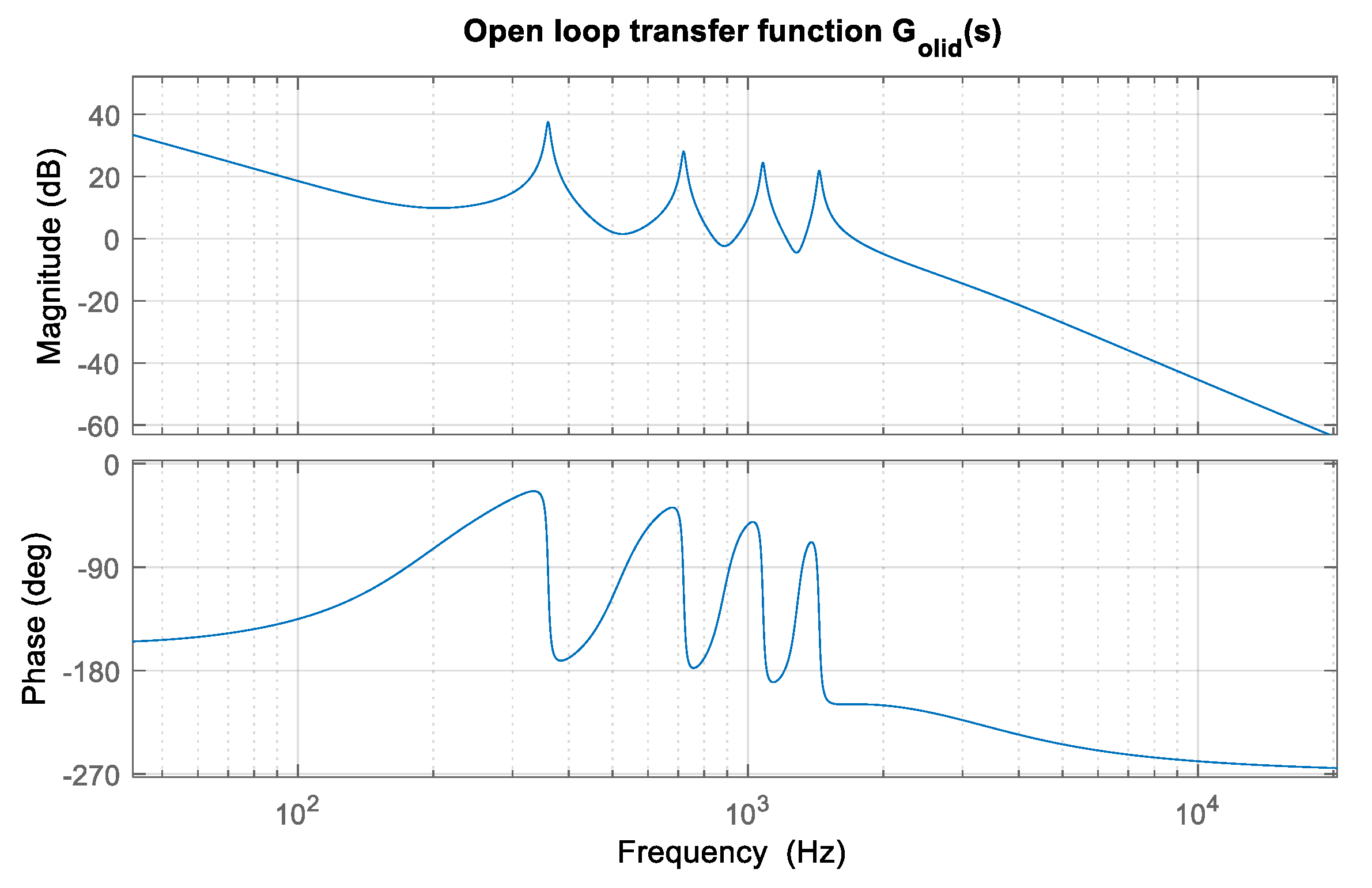
where ${MFk}_{DC}=tan\left({PM}_{VCD}-\pi \right)$. The design characteristics of the controller are selected considering the desired response speed of the control of the current loops and the voltage loop within the criteria presented above. The values obtained for the controllers are shown by

Table 1. Controller parameters.

Controller	Design Parameter	Controller Gain
Current Loop	Phase margin PMic = 65° Crossover frequency ωic = 600 Hz	Kp = 8.61 Ki = 1.447 × 104
Voltage Loop	Phase margin PMVCD = 70° Crossover frequency ωVCDc = 30 Hz	Kp = 0.93 Ki = 62.1

, as well phase margins and crossover frequencies, where a frequency response ten times above the frequency of the fundamental was chosen. The voltage loop controller was proposed so that the recovery time from a transient is approximately one cycle of the voltage period. The diagram of Bode is shown by Figure 3.

5.2. Resonant Controller Design

The compensated equivalent harmonics in the synchronous reference frame are those with a frequency 6000 times the fundamental frequency. There are different design methods for Proportional+Resonant (PR) type controllers. In [27], a modification of the Ziegler Nichols method is used. In [15,30], the gains are obtained by adjusting the distance to the critical point; this is the method used for designing the proposed PI+Resonant controller. When the tuning is done by adjusting the distance to the critical point (−1, j0), the stability of the control loop must be verified; this is accomplished using the Nyquist stability criteria for systems with delay [31]. The previously obtained gains of K_p and K_i are used to limit the degrees of freedom of the controller, to easily obtain a range of values of each resonant controller K_Rn, maintaining the current loop in steady state, where the critical point is not encircled. Next, the sensitivity function of the system is used.

$$S_0\left(s\right)=\frac{1}{{1+G}_{olidq}\left(s\right)},$$

(29)

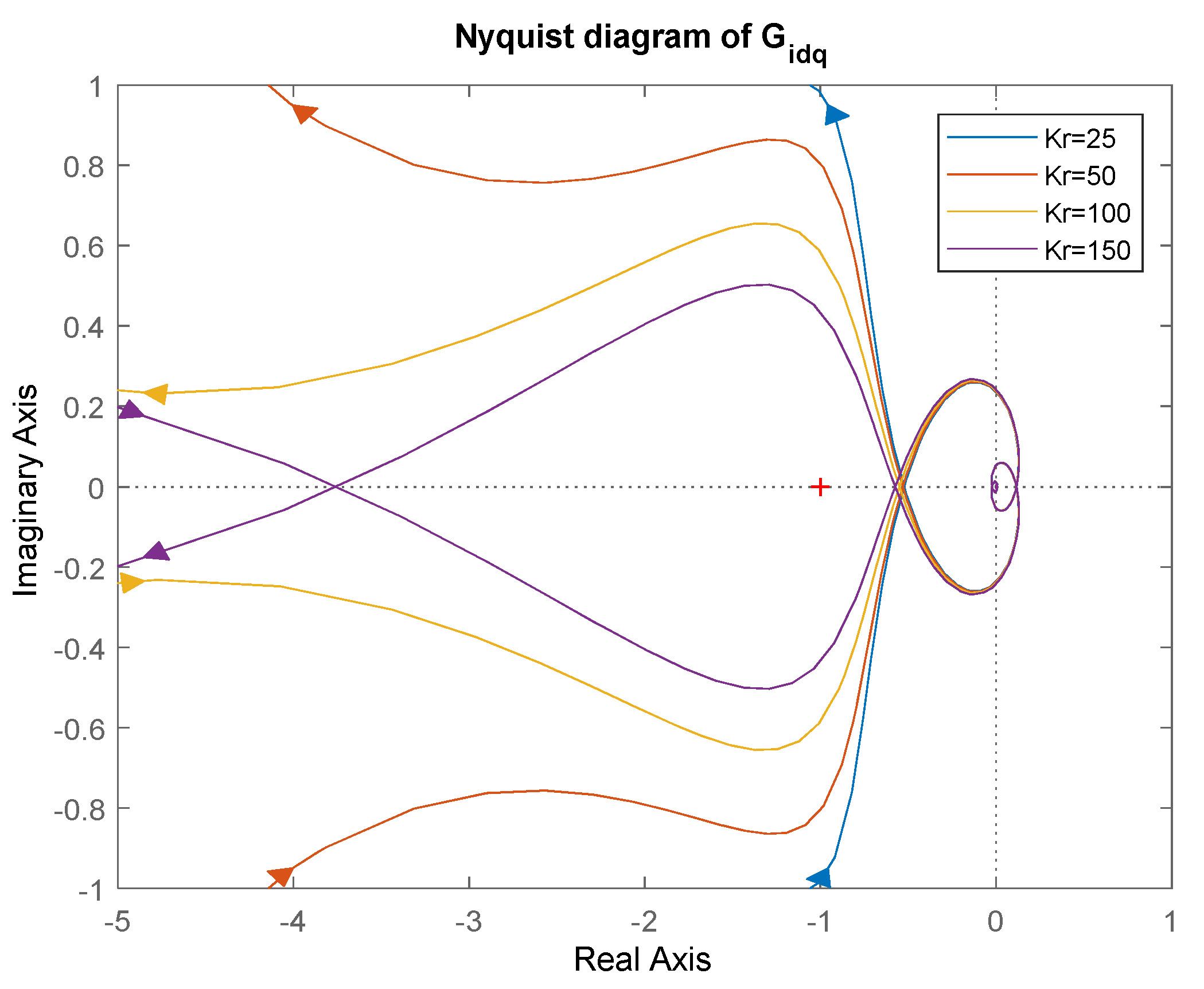
The calculation of the resonant controller gains is carried out using a Nyquist graph, considering a minimum distance η₀ to the critical point:

$$\frac{1}{{\eta }_0}=\underset{0\le \omega <\infty }{max}\left|S_0\left(j\omega \right)\right|=\Vert S_0\left(s\right)\Vert {}_{\infty }.$$

(30)

Setting η₀ = 0.1 and ξ = 0.01 and taking into account a measured delay of 300 μs, the analysis is performed for each frequency. The K_Rn values that present the best response, for each of the equivalent harmonic frequencies, in the dq reference frame are shown in

Table 2. Gains of the controllers for each harmonic order.

Harmonic Order	Gain
6	Kr6 = 100
12	Kr12 = 80
18	Kr18 = 80
24	Kr24 = 80

. Figure 4 shows the Nyquist plot of the PI+Resonant controller for the 6th harmonic, where the corresponding trajectories are observed at different gains; in this case, for the gain K_r = 150, it is observed that the path encloses the critical point. Therefore, a value of K_r = 100 is selected, verifying that the minimum distance is maintained η₀ at this point.

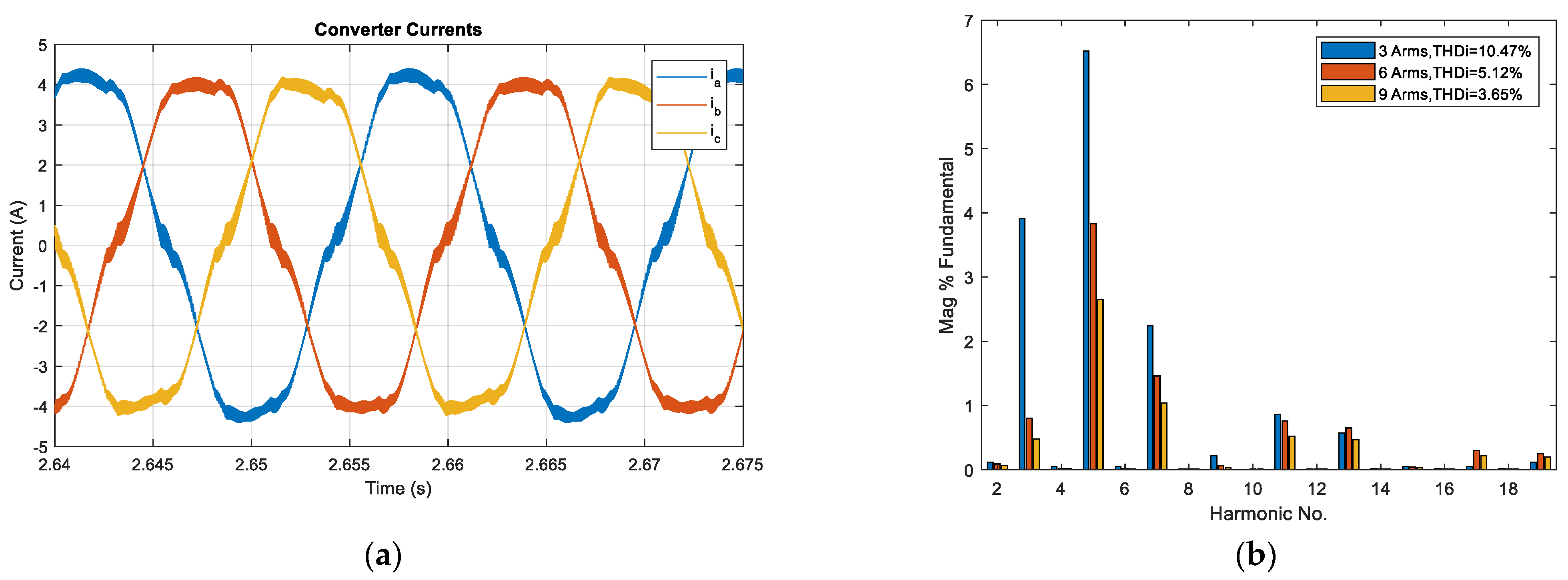
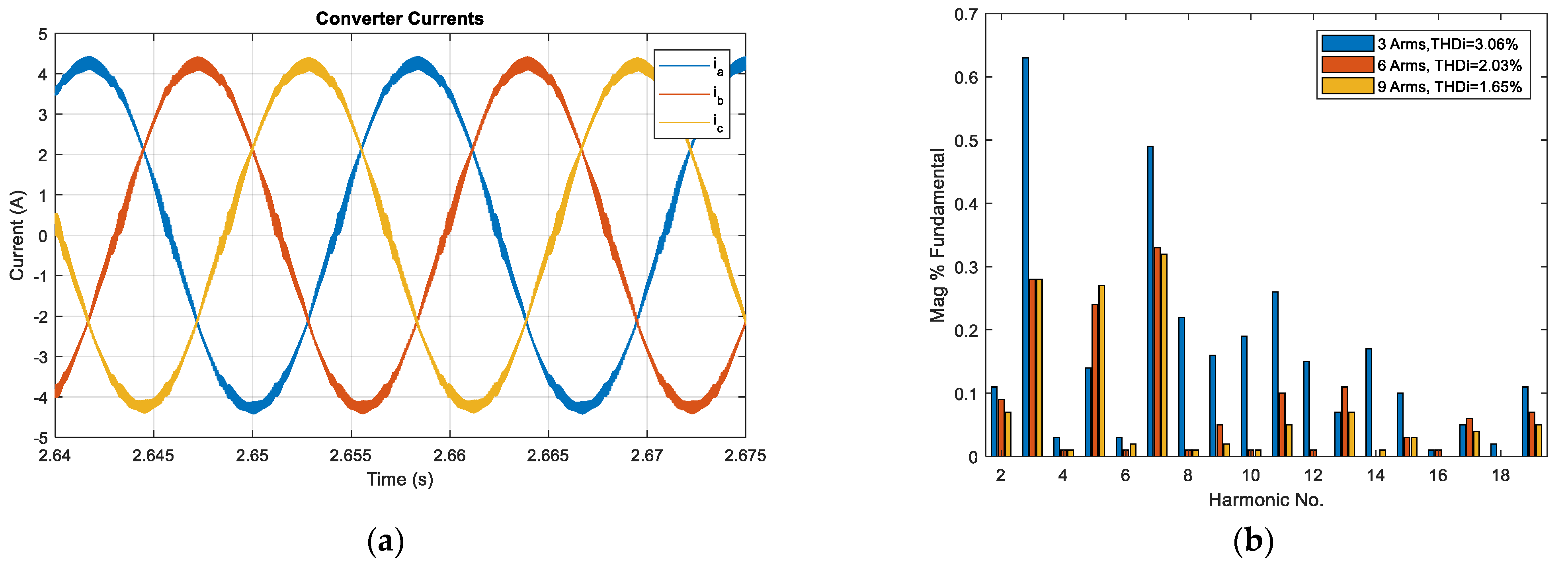
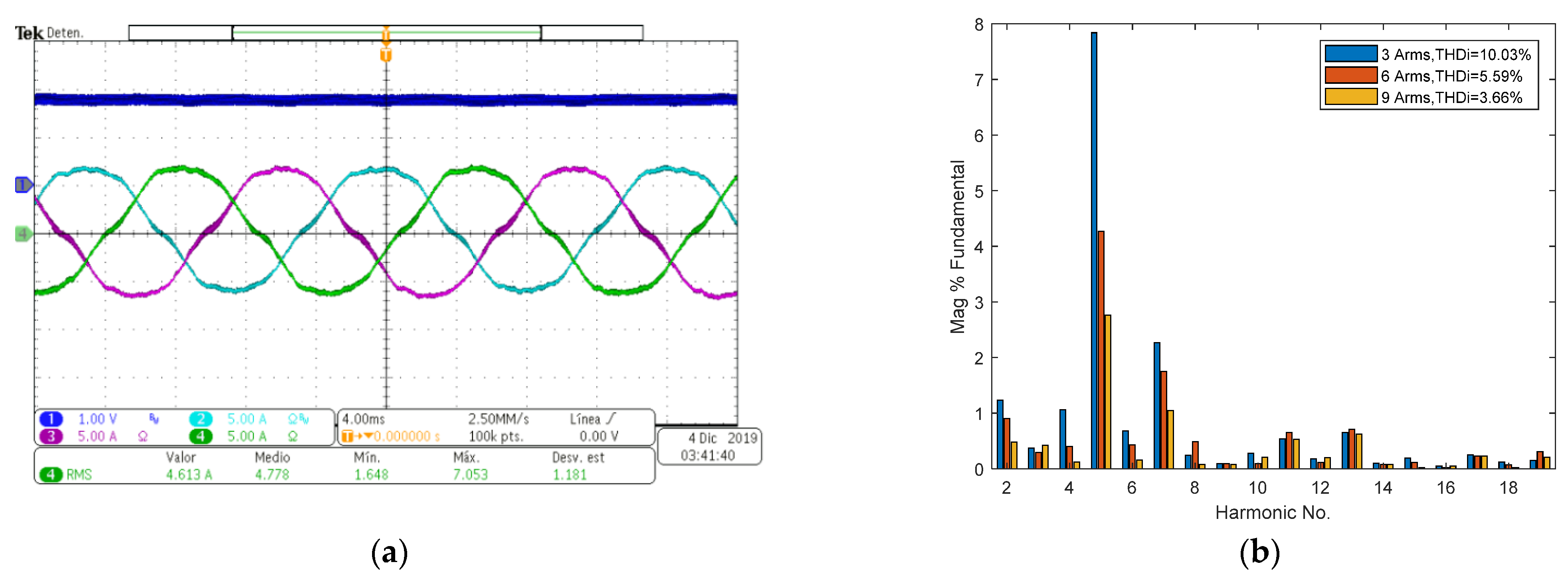
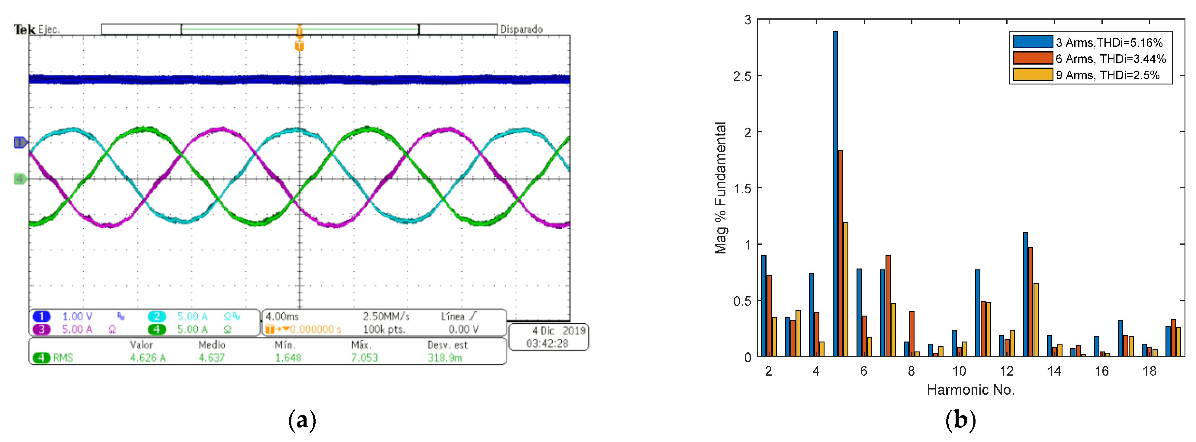
With the analysis of simulated and experimental results with a classical PI controller on the converter, it was found that harmonics higher than the 24th have an amplitude less than 0.5% of the fundamental, so its contribution to increase the overall harmonic distortion in the current (THDi) has little impact. In addition, amplitudes below 0.5% in the harmonics >24 are compliant with the standard 1547–2018. For this reason, the resonant controllers were designed for odd harmonics up to order 24, excluding the zero-order ones.

6. Digital Implementation

The digital implementation of the controller was done by discretizing the controllers using the Tustin approximation considering a sampling period of T_s = 5 µs. The discretized PI controller has the form:

$$H_{id}\left(z\right)=K_p+\frac{K_i{T}_s}{2}\frac{1+z^{-1}}{1-z^{-1}}.$$

(31)

The discrete resonant controllers for each frequency are expressed by:

$$H_{k,6}\left(z\right)=\frac{0.2255z-0.2255}{z^2-1.985z+0.9977},$$

(32)

$$H_{k,12}\left(z\right)=\frac{0.358z-0.358}{z^2-1.945z+0.9955},$$

(33)

$$H_{k,18}\left(z\right)=\frac{0.5307z-0.5307}{z^2-1.88z+0.9932},$$

(34)

$$H_{k,24}\left(z\right)=\frac{0.6962z-0.6962}{z^2-1.791z+0.991}.$$

(35)

7. Experimental Setup and Results

The prototype of the back to back converter used in the experimental verification is shown in Figure 5. The control algorithm was implemented in a Delfino F28335 evaluation board, which implements the digital signal processor (DSP) TMS320F28335, a 32 bit single precision floating point unit, with a processing capability of 150 MIPS (million instructions per second). The converter uses a FNA25060 IGBT intelligent module, with a maximum current of 30 A. The design characteristics of the converter are shown in

Table 3. Inverter and filter parameters.

Title 1	Title 3
RMS line voltage	110 V
Nominal power	5.76 kVA
DC bus reference voltage	190 V
RMS rated current	30 A
Capacitor on the DC Bus	5.4 mF
Inductor L	2.5 mH
Resistance of the inductor rL	65 mΩ

. The converter operates at a switching frequency of 20 kHz, and a dead time of 2 µs is required by the IGBTs of the converter. Measurements are performed using the Hall effect voltage sensors LV25–P and the current sensor LTSR 25–NP. The experimental measurements were made with a Tektronix MDO3014 100 MHz 2.5 Gs/s oscilloscope, with 4 channels, Tetronix current probes, and a Hioki PW3198 power analyzer. The inductor used is a three-phase line reactor, with an inductance per phase of 2.5 mH and a resistance in the windings of 160 mΩ. The converter is connected to the secondary of a 220 V to 110 V, 7.5 kVA step-down transformer.

7.1. Simulation Results

Simulation results were obtained with a simulation model in the Simulink™ GUI of the numerical software Matlab © to evaluate the performance of the implemented PI+Resonant controllers when compensating for the converter and grid harmonics. The three-phase grid voltages are simulated reproducing the conditions in the laboratory; this is done by recording the line voltages in a time interval of 20 s and used in simulation to replicate the real conditions of the grid in the laboratory. The three–phase voltages of the laboratory have an amplitude unbalance of 2.2% in one of its phases and a voltage THD of 1.82%.

Dead times were included in the simulation, as well as the parasitic resistances of the inductors. Additionally, a Space Vector Pulse Width Modulation (SVPWM) algorithm was implemented. To validate the results obtained using the proposed PI+Resonant controller, tests were compared with the results of a traditional PI controller. The tests are performed by applying a constant current load on the DC bus to demand 3, 6, and 9 A currents on the grid side. Figure 6 shows the behavior of the currents when using a conventional PI controller. Figure 6a shows the waveform of the currents when 3 A are demanded, where a THDi of 10.47% is obtained. Figure 6b shows the harmonic content of the converter currents for the values 3, 6, and 9 A, where the THDi decreases as the load current is increased. Figure 7 shows the currents’ behavior when the proposed PI+Resonant controller is used. Figure 7a shows their correspondent waveforms when a load of 3 A is demanded, where a THDi of 3.06% is obtained. Figure 7b shows the harmonic content of the converter currents for the values 3, 6, and 9 A, where it is observed that the THDi also decreases as the current demand increases.

7.2. Experimental Validation

The experimental results were obtained using the same grid voltage conditions used in the simulation (THD 1.82%, and an imbalance in one of the phases of 2%). The same tests were carried out as in the simulation; for a conventional PI, the total harmonic distortion of the current is 10.03% at 3 A, and its waveform is shown by Figure 8a. The harmonic content for a current sweep of 3, 6, and 9 A is shown by Figure 8b, where a considerable amplitude is observed in the fifth harmonic. When the PI+Resonant controller is used, a THDi of 5.16% is obtained at 3 A; Figure 9a shows its current waveforms. The current harmonic sweep is shown by Figure 9b; in this case, there is a considerable reduction at the fifth harmonic, which is compliant with the 1547–2018 standard.

7.3. Reactive Power Injection in the Wind Generation System

The reactive power controller was implemented to allow the converter to inject or demand reactive power, according to the reactive power reference $Q_c^{*}$ given by the user according to the grid requirements, and the current reference $i_q^{*}$. is calculated according to the analysis in Section 4. Figure 10 shows a step of Q_c = 3000 VAR, which is followed by a transition to Q_c = −3000 VAR.

7.4. Discussion of the Results

According to the IEEE 519–2014 standard, the harmonic distortion in the current is designated with the total demand distortion (Total Demand Distortion (TDD)), which measures the harmonic content with respect to the maximum RMS current. The standard 1547–2018 introduces the new term, Total Rated Current Distortion (TRD), which is used for Distributed Energy Resources (DER). The standard 1547–2018 states that TRD values must be less than 5%. Considering values of TRD less than 5%, when the RMS value of the current fundamental component approaches the RMS value of the rated current of the installation $I_{Lrated}\approx I_{1,L}$, the consideration THDi ≈ TRD can be done. For the converter operating at nominal load, THDi values lower than 2.5% are obtained, which are within the permitted values for power generation systems; however, the tests that were carried out (Figure 8 and Figure 9) correspond to a current sweep where the smallest value (3 Arms) presented the largest distortion (10.03%), and the distortion decreases as the currents increases, where above 9 Arms, the distortion goes below 2.5%, due to the increase in the magnitude of the fundamental with respect to the high frequency ripple, which impacts the sensitivity of the current control loop, when the system demands small currents. It is important to mention that the TRD refers to the nominal current of the converter; therefore, this value will be higher when the distortion high for currents close to the nominal value. It is important to mention that with regard to the reactive power control on the GSC, the total reactive power of the WGS can be controlled on the DFIG stator as well. When combined, the WGS can control a higher reactive power when the reactive power generated by the machine is insufficient to supply the demand.

8. Conclusions

This paper presents the implementation of resonant controllers on the synchronous reference frame (dq) for the grid side Converter in a wind generation system. The resonant controllers are added in parallel to the PI controller at a current control loop. The tuning process of this control loop was is performed in two steps. The first step is tune the gains of the PI controller the same way as is done in classic control, and the second step is to tune the resonant controller by finding the range where the resonant gains maintain the minimum distance to the critical point and adjusting them to achieve the best performance tracking the harmonic components. The proposed resonant controllers achieve an important improvement in the THDi; the THDi obtained is 3.65% in the simulated results and 5.16% in the experimental results. Four resonant controllers were implemented to reduce harmonics from sixth up to the 24th on the synchronous reference frame dq. The resonant controllers on the synchronous reference behave as double integrators when implemented in both axes of the dq coordinated system, allowing the controller to track the frequency pairs (1 + 6k) and (1 − 6k) by taking advantage of the frequency shift of the park transformation. Moreover, its implementation requires less computational cost from the DSP, because the proposed controllers use simple arithmetic compared to the high computational cost when nonlinear control is used due to the nature of the mathematical operations involved in this type of algorithm.