Sensorless PMSM Drive Inductance Estimation Based on a Data-Driven Approach

Abstract

In the permanent magnet synchronous motor (PMSM) sensorless drive method, motor inductance is a decisive parameter for rotor position estimation. Due to core magnetic saturation, the motor current easily invokes inductance variation and degrades rotor position estimation accuracy. For a constant load torque, saturated inductance and inductance error in the sensorless drive method are constant. Inductance error results in constant rotor position estimation error and minor degradations, such as less optimal torque current, but no speed estimation error. For a periodic load torque, the inductance parameter error periodically fluctuates and, as a result, the position estimation error and speed error also periodically fluctuate. Periodic speed error makes speed regulation and load torque compensation especially difficult. This paper presents an inductance parameter estimator based on polynomial neural network (PNN) machine learning for PMSM sensorless drive with a period load torque compensator. By applying an inductance estimator, we also proposed a magnetic saturation compensation method to minimize periodic speed fluctuation. Simulation and experiments were conducted to validate the proposed method by confirming improved position and speed estimation accuracy and reduced system vibration against periodic load torque.

1. Introduction

Permanent magnet synchronous motors (PMSMs) are largely applied to home appliances and automotive motors owing to their high efficiency and lightweight features. For a high performance PMSM drive, a rotor field-oriented control method is widely used. In this method, accurate position information of the rotor must be identified in real time. However, because of realistic problems, such as inability to mount, cost, and faulty situation of sensors, studies are actively being conducted on sensorless control methods that estimate rotor position and speed without a directly mounted position sensor [1,2,3,4,5,6]. The synchronous reference frame model-based sensorless control method is largely classified into current model-based and extended electromotive force (EMF)-based methods [2,3]. Currently, the latter method is commonly used because of its fast-tracking capability using the arc-tangent calculation.

To estimate the rotor position, the model-based sensorless control method utilizes motor parameters of inductance, resistance, and back EMF constant. Hence, motor parameter errors deteriorate the position estimation error and, as a result, degrade the control performance of the system. Particularly in environments where the motor drive is directly exposed to a periodic load torque, such as pumps, home appliance compressors, and vibration suppressors injecting counter motor torque, the control performance can be significantly compromised. In these cases, the effects of load torque fluctuation can be counteracted by analyzing the load pattern and applying a proper compensation current [7,8,9]. However, using this load torque compensation method reduces the effects of fluctuating load torque, and the magnitude of compensation torque current is increased. This leads to a secondary problem in speed estimation error due to magnetic saturation. The core saturation invokes inductance reduction, which creates an inductance parameter error in rotor position estimation by the sensorless control method. If the load torque is constant, the torque current and the inductance parameter error from the core saturation are constant values and the rotor position estimation error is constant. This constant rotor position error does not invoke a speed estimation error; it only invokes minor degradations such as a less optimal torque current. However, when the load torque has a periodic component, the inductance parameter error has a periodic fluctuation and periodic components in the speed error and position estimation error occur. The periodic speed error results in difficulty in speed regulation and load torque compensation. As a result, severe mechanical noise and vibrations still exist. If a proper compensation method considering this problem is not implemented, mechanical instability of the entire system as well as noise, vibration, and harshness (NVH) problems could be present. By accurately estimating the actual value of inductance, the accuracy of sensorless speed control can be improved [10,11,12,13].

To compensate for the magnetic saturation problem, inductance estimation studies have been conducted with mathematical models, such as a flux observer [13,14,15,16,17]. However, the sensorless drive method utilizes an identical PMSM model to estimate the rotor position. The model-based flux observer utilizes the estimated rotor position and speed from the sensorless drive method. Hence, the inductance estimator is sensitive to the back EMF constant and drive output voltage error. Even with a well-tuned back EMF constant, the estimated inductance could worsen system stability and speed estimation error, particularly for periodic load torque fluctuation.

As a parameter estimator, a data-driven approach based on soft computing method can be used since estimation can be done with the selected input data while excluding any model parameters. In comparison to mathematical model-based methods, data-driven approaches, such as machine learning approach, are more appropriate to learn the predictive model for unknown parameter estimation [18]. With a recursive training process, the input data errors, which include inverter output voltage error, current sensor offset, and various nonlinear components, can be excluded. Moreover, this method can learn parameters faster and more accurately in a nonlinear relationship where the input and output relationship, or functional type of the model, is uncertain. In particular, the polynomial neural network (PNN)-based group method of data handling (GMDH) estimates output parameters with a polynomial expression of multiple layers. It has fast calculating speed, good real-time performance, and excellent accuracy. Moreover, it has many advantages when applied to an embedded system compared to a neural network, fuzzy logic, etc. It could effectively reduce estimated parameter errors by training the network as it combines multiple input/output data to dynamically estimate the collections of necessary factors [19,20]. Recent studies have applied machine learning to the motor control system to exploit these advantages. However, to our knowledge, there has been no attempt to apply PNN-based machine learning for the prediction of sensorless control parameters and compensation control because of difficulty in implementation, optimization, etc. [21,22]. In particular, if the design factors are not properly selected when applying a PNN-based learning method to a nonlinear system, the control characteristics of the system could be degraded, and the entire system can become unstable if an unexpected disturbance or fault occurs. Therefore, it is necessary to design and optimize a suitable method for the sensorless nonlinear system and to have a quick-response control strategy when errors or faults occur during parameter estimation.

Comparing to the conventional model-based inductance estimation, the PNN-based estimation has the following list of major advantages for a PMSM sensorless system. Firstly, the PNN-based learning method is suitable for complex nonlinear models—it can reduce the cost for a fine tuning of a variety of PMSM sensorless systems. Secondly, the PNN-base learning method accurately estimate the unknown parameter and compensates without delay or distortion. Hence, it performs better than the other methods in terms of root mean square error (RMSE) and correlation coefficients. Thirdly, it can be easily adaptable to various operating load condition including step, periodic, and random profiles with the learning process.

In this paper, the $q$-axis inductance estimation method for a sensorless PMSM drive is studied to minimize rotor position and speed error and compensate external periodic load torque variation. To minimize the uncertainty based on magnetic saturation and improve real-time control performance, we proposed a PNN-based compensation method using a GMDH algorithm to estimate the $q$-axis inductance and perform compensation control for magnetic saturation. In addition, to reduce the estimation error and improve control accuracy, an optimization learning of the $q$-axis inductance parameter was conducted with respect to various load torque patterns. To effectively respond to fault situations, such as unexpected disturbances or errors in estimated values, the position error was also estimated and monitored in real time. A software simulation was performed on a sensorless PMSM drive to validate the proposed PNN-based compensation method and confirm the result of the control performance. Through the experiment, we confirmed that sensorless speed estimation error is reduced with PNN-based inductance and frequency response characteristics of the system. The NVH performance was also improved.

2. Extended EMF-Based Sensorless Control

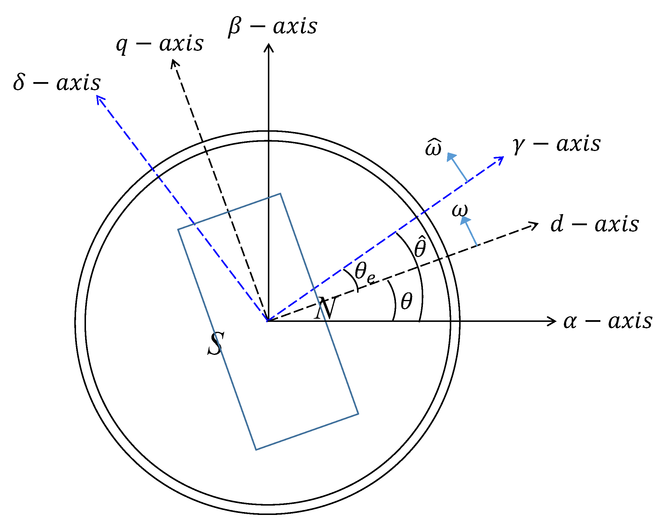
Figure 1 shows a space vector diagram of a PMSM. Note that $\alpha$-$\beta$, $d$-$q$, and $\gamma$-$\delta$ represent two axes in the stationary reference frame, the synchronous reference frame, and the estimated frame for a sensorless control, respectively. ${\theta }_e$ is the difference between the actual rotor position $\theta$ and the estimated rotor position $\widehat{\theta }$. $\omega$ and $\widehat{\omega }$ denote the actual and the estimated rotor speed, respectively. The voltage equation in $d$-$q$ synchronous frame is given by

$$\left[\begin{array}{c}{v}_d\\ v_q\end{array}\right]=\left[\begin{array}{cc}{R}_a+p{L}_d& -\omega L_q\\ \omega L_q& R_a+p{L}_d\end{array}\right]\left[\begin{array}{c}{i}_d\\ i_q\end{array}\right]+\left[\begin{array}{c}0\\ \omega \psi \end{array}\right],$$

(1)

where $R_a,L_d,L_q,$ and $\psi$ represent the stator resistance, the $d$-$q$ axes inductance, and the back EMF constant, respectively; $p$ is a differential operator; $v_d$, $v_q$, and $i_d$, $i_q$ are the stator voltage and current in the $d$-$q$ synchronous reference frame, respectively.

Ignoring the difference between the estimated speed and the actual speed, (1) can be converted to the $\gamma$-$\delta$ axes estimated by the extended back EMF. Then, the voltage equation can be represented as [2]

$$\left[\begin{array}{c}{v}_{\gamma }\\ v_{\delta }\end{array}\right]=\left[\begin{array}{cc}{R}_a+p{L}_d& -\omega L_q\\ \omega L_q& R_a+p{L}_d\end{array}\right]\left[\begin{array}{c}{i}_{\gamma }\\ i_{\delta }\end{array}\right]+\left[\begin{array}{c}{e}_{\gamma }\\ e_{\delta }\end{array}\right],$$

(2)

where $e_{\gamma }=-E_{ex}\sin {\theta }_e, e_{\delta }=-E_{ex}\cos {\theta }_e, and E_{ex}=\omega \left[\left(L_d-L_q\right)i_d+\psi \right]-\left(L_d-L_q\right)\frac{d{i}_q}{dt}$. $v_{\gamma }$, $v_{\delta }$, $i_{\gamma }$, $i_{\delta }$, $e_{\gamma }$, and $e_{\delta }$ are the stator voltage, the current, and the extended back EMF in the $\gamma$-$\delta$ estimated synchronous reference frame, respectively, which includes rotor position error. Using $e_{\gamma }$ and $e_{\delta }$, the rotor position error can be calculated as

$${\widehat{\theta }}_e={\tan }^{-1}\left(-\frac{{\widehat{\theta }}_{\gamma }}{{\widehat{\theta }}_{\delta }}\right)\cong -\frac{{\widehat{e}}_{\gamma }}{E_{ex}}.$$

(3)

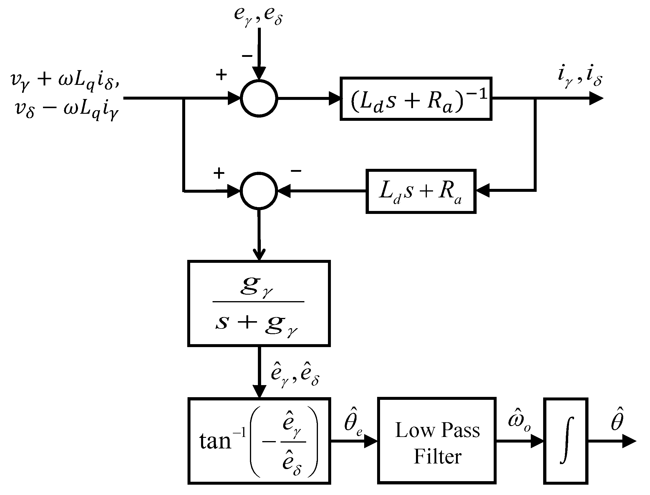
As shown in Figure 2, the estimated speed $\widehat{\omega }$ can be obtained through the PI controller that takes the estimated rotor position error ${\widehat{\theta }}_e$ as an input. Finally, the rotor position $\widehat{\theta }$ can be estimated by integrating the estimated speed.

3. Compensating Method for Magnetic Saturation

3.1. Analysis of Inductance Saturation Effect on Sensorless Control

For precise rotor position estimation in sensorless control, the accuracy of parameters, such as resistance and inductance in (2), is important. In a system with a large periodic load, such as a pump or compressor, if the error between the actual $q$-axis inductance ($L_q$) and the estimated $q$-axis inductance (${\widehat{L}}_q$) increases due to magnetic saturation, the estimated rotor position becomes inaccurate. Considering the error between the actual value and the estimated value due to magnetic saturation, (2) can be reorganized for the extended back EMF, $e_{\gamma }$ and $e_{\delta }$, which are expressed as

$$\left[\begin{array}{c}{e}_{\gamma }\\ e_{\delta }\end{array}\right]= \left[\begin{array}{c}{v}_{\gamma }\\ v_{\delta }\end{array}\right]-\left[\begin{array}{cc}{R}_a+p{L}_d& -\omega {\widehat{L}}_q\\ \omega {\widehat{L}}_q& R_a+p{L}_d\end{array}\right]\left[\begin{array}{c}{i}_{\gamma }\\ i_{\delta }\end{array}\right]+\left[\begin{array}{c}\Delta e_{\gamma }\\ \mathsf{\Delta }{e}_{\delta }\end{array}\right]$$

(4)

where $\mathsf{\Delta }{e}_{\gamma }=-p\mathsf{\Delta }{L}_d{i}_{\gamma }+\omega \mathsf{\Delta }{L}_q{i}_{\delta }$ and $\mathsf{\Delta }{e}_{\delta }=-p\mathsf{\Delta }{L}_d{i}_{\delta }-\omega \mathsf{\Delta }{L}_q{i}_{\gamma }$. Note that $\mathsf{\Delta }{L}_d$ and $\mathsf{\Delta }{L}_q$ are the parameter errors of $d$- and $q$-axes inductance, respectively, which are obtained by subtracting the estimated inductance from the actual inductance $(\mathsf{\Delta }{L}_d=L_d-{\widehat{L}}_d$, $\mathsf{\Delta }{L}_q=L_q-{\widehat{L}}_q)$. The rotor position error is influenced by the inductance error.

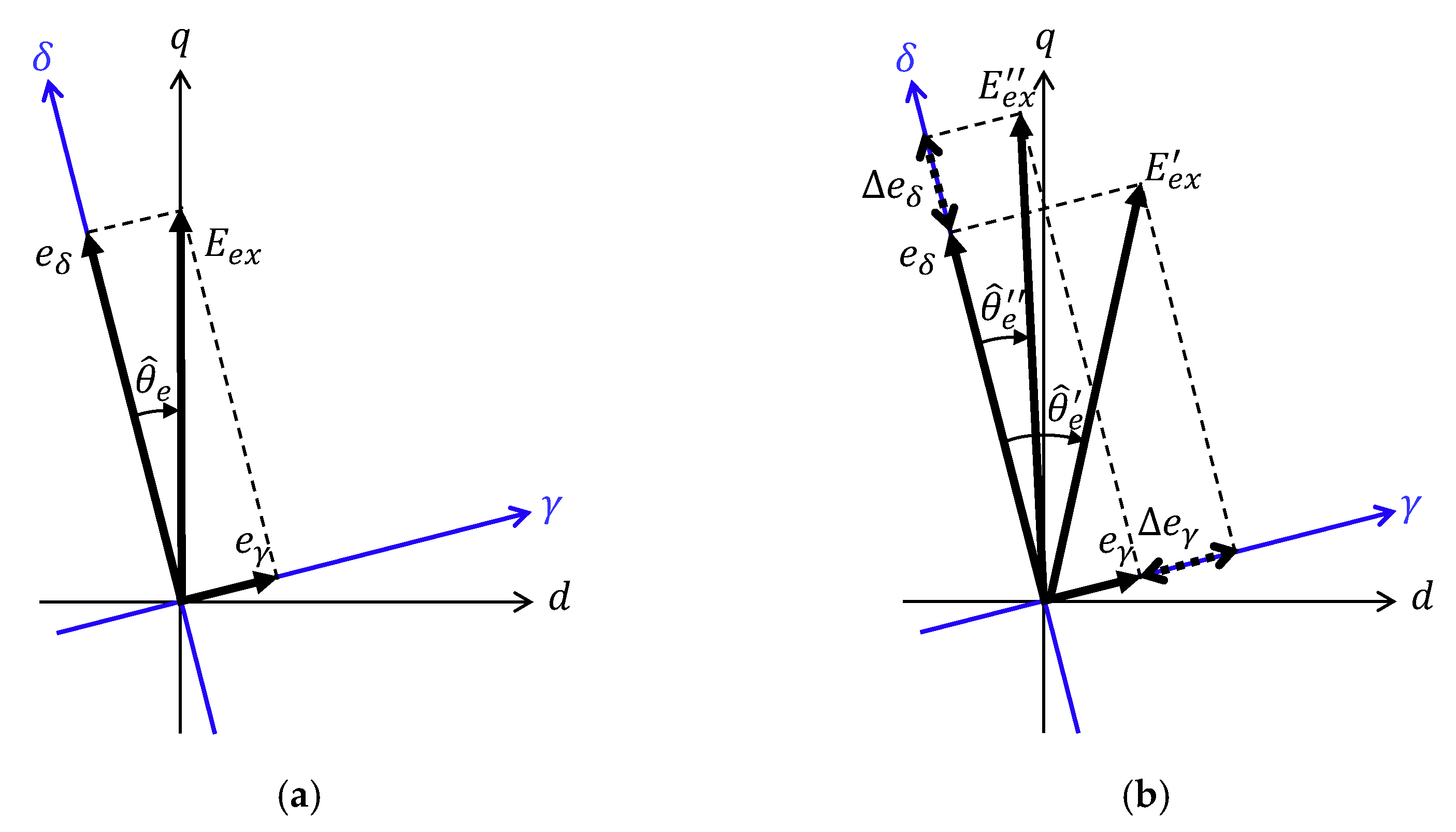
Figure 3 shows a comparison of estimated rotor position error according to the voltage error of the $\gamma$-$\delta$ axes extended back EMF. Note that ${\widehat{\theta }}_e^{\prime }$ and $E_{ex}^{\prime }$ are the estimated rotor position error and the extended EMF due to the $\gamma$-axis extended back EMF error ($\Delta e_{\gamma }$), respectively. ${\widehat{\theta }}_e^{″}$ and $E_{ex}^{″}$ are the estimated rotor position error and extended EMF due to the $\delta$-axis extended back EMF error $(\Delta e_{\delta }$), respectively. In Figure 3a, when the extended back EMF, $e_{\gamma }$ and $e_{\delta }$, are constant without error, the estimated extended EMF coincides with the $d$-$q$ synchronous reference frame. However, when the variation of the $\gamma$-$\delta$ axes’ extended back EMF occur due to an inductance variation, as a result, the estimated rotor position error varies, as shown in Figure 3b. Typically, since the $\delta$-axis extended back EMF, $e_{\delta }$, includes the back EMF voltage, it is larger than the $\gamma$-axis component ($e_{\gamma }\ll$ $e_{\delta }$). Hence, the $\gamma$-axis extended back EMF variation has a dominant effect on the estimated rotor position error and estimated speed compared to the $\delta$-axis component when the magnitudes of $\Delta e_{\gamma }$ and $\Delta e_{\delta }$ are the same.

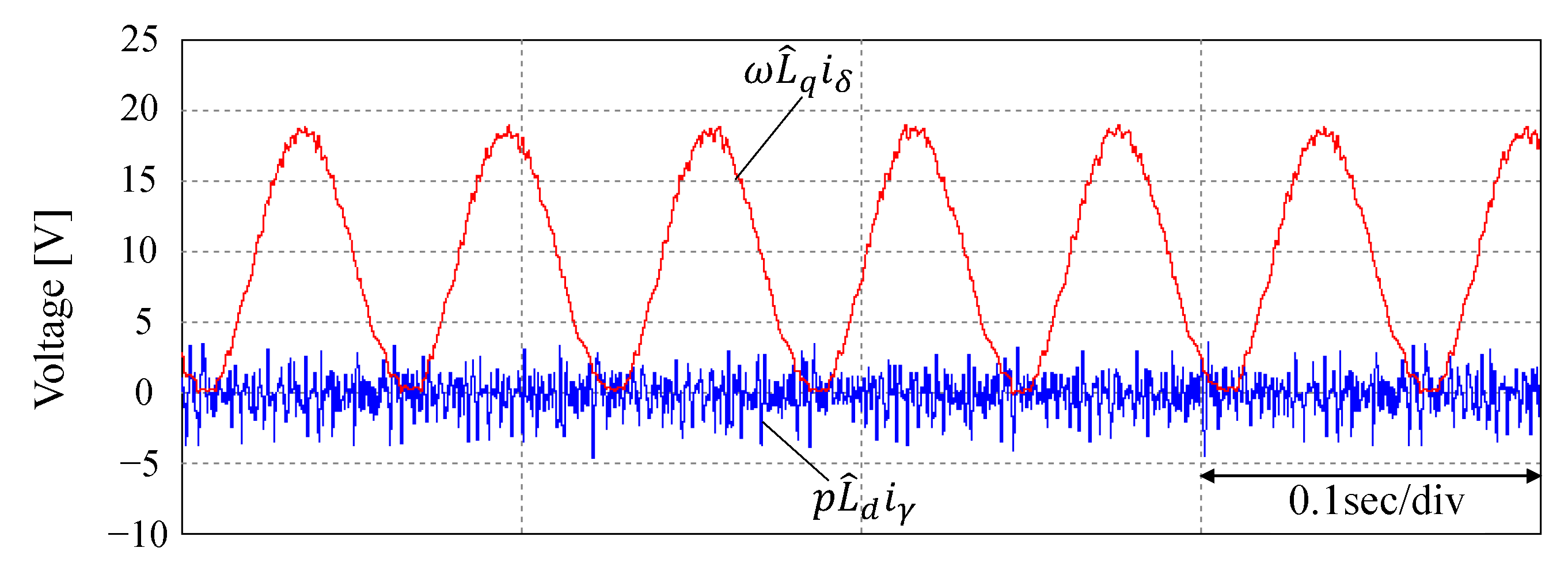
In Figure 4, simulation plots of $\omega {\widehat{L}}_q{i}_{\delta }$ and $p{\widehat{L}}_d{i}_{\gamma }$ are shown under a periodic load torque (16.6 Hz). Since $L_q$ and $i_{\delta }$ are conventionally larger than $L_d$ and $i_{\gamma }$, respectively, $\omega {\widehat{L}}_q{i}_{\delta }$ has a much larger magnitude than $p{\widehat{L}}_d{i}_{\gamma }$ in Figure 4. In the same manner, the dominant component of $\mathsf{\Delta }{e}_{\gamma }=-p\mathsf{\Delta }{L}_d{i}_{\gamma }+\omega \Delta L_q{i}_{\delta }$ is $\omega \mathsf{\Delta }{L}_q{i}_{\delta }$, and it can be assumed that $\mathsf{\Delta }{e}_{\gamma }\approx \omega {\mathsf{\Delta }L}_{\mathrm{q}}{i}_{\delta }$. Hence, if the $q$-axis inductance $L_q$ is accurately estimated, the rotor position error and speed error can be minimized. However, since $L_q$ is easily saturated by the $q$-axis current, it makes rotor position estimation difficult. This is especially true under a periodic load torque; the $q$-axis current has a periodic variation to regulate the motor speed. The periodic $q$-axis current creates periodic $q$-axis inductance variation from core magnetic saturation. As a result, the rotor position error has a periodic component and, moreover, speed error exists.

3.2. Model-Based Inductance Estimation Method

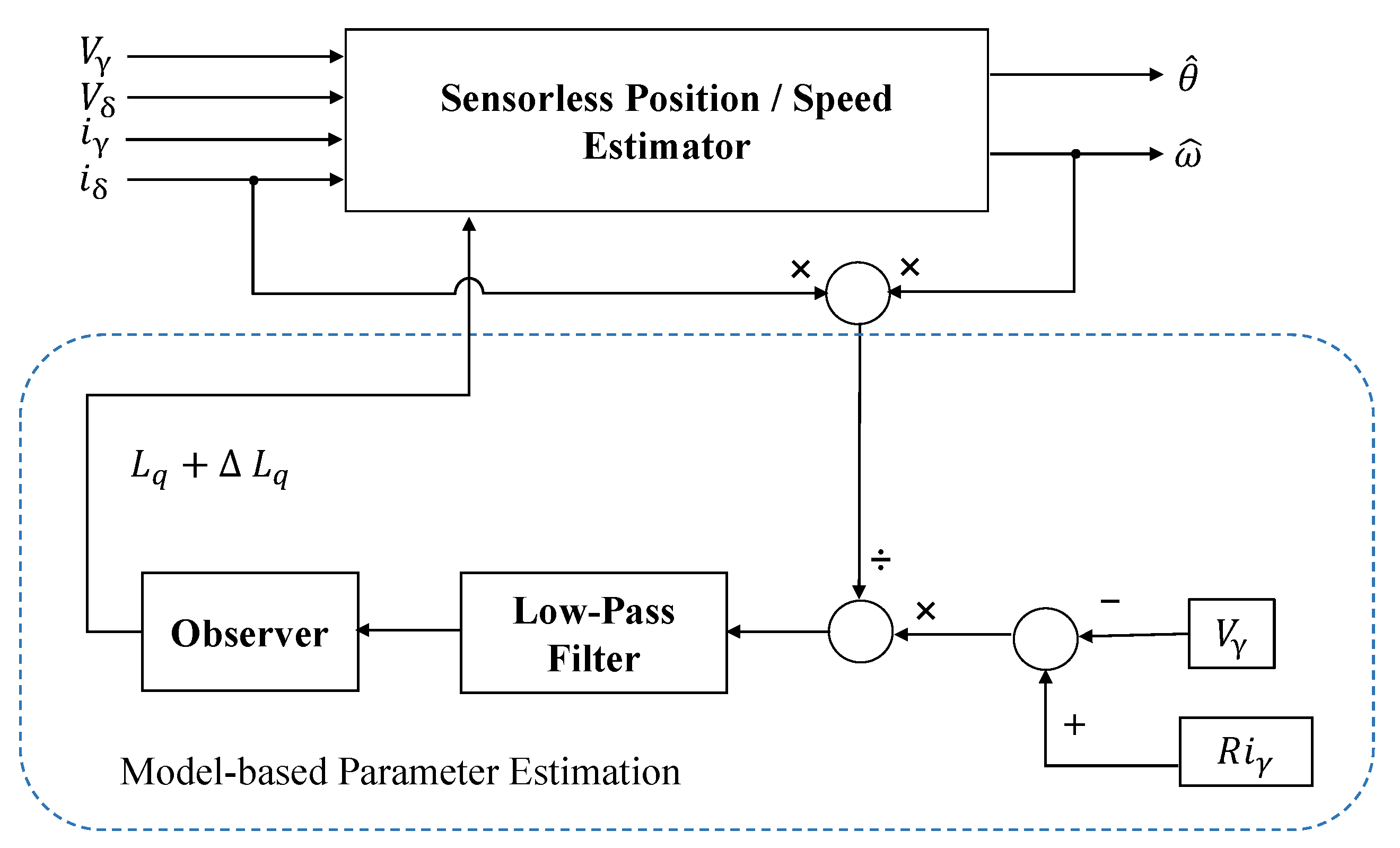
In most conventional model-based inductance estimation methods, the inductance estimated by a model-based observer is fed back to the sensorless controller and compensates the magnetic fluctuation [13,14,15,16,17]. From (1), the differential components can be ignored by assuming a steady-state condition. Then, the $d$- and $q$-axes inductance can be represented as

$$\{\begin{array}{l}{L}_q=\frac{-v_d+R_s{i}_d}{\omega i_q}\hfill \\ L_d=\frac{-v_q+R_s{i}_q+\omega {\psi }_f}{\omega i_q}\hfill \end{array}.$$

(5)

Figure 5 shows a block diagram of the $q$-axis inductance estimator based on (5). In this parameter estimator model, a low-pass filter is required to minimize undesired high-frequency noise and ripple. However, a time delay and a DC offset due to the integral function are inevitable when applying the low-pass filter. Therefore, in a system exposed to a large amount of dynamic load, a compensator, such as a time delay compensator, is required. In addition, the angular speed, which is a variable estimated by the sensorless control observer, is reused for estimating the inductance parameter. Thus, when the estimated speed errors increase, the estimated inductance becomes inaccurate and the speed control also becomes unstable.

Figure 6 shows the simulation results of the step response with the observer model-based inductance estimator. If a transient load is applied in this system, a time delay and DC offset occur, resulting in more than 5% error compared to the actual value.

4. Proposed Inductance Estimation Method

With the model-based $q$-axis inductance estimation method, it has a limitation that the estimation error could worsen system stability and accuracy, since the estimator is sensitive to errors of inverter nonlinearity, rotor position, and motor parameters. The PNN-based estimation method studied in this study is in the form of a “black box” in which everything such as voltage/current errors are already included, and the errors can be minimized by repetitive training.

4.1. Data-Driven Approach for Inductance Estimation

On the one hand, since both the extended EMF sensorless control and the model-based inductance estimation utilize the same motor dynamics, the response speed of the estimated rotor position and inductance are partially contradicted, and a time delay is created. On the other hand, the PNN-based machine learning method predicts a system equation by selecting input variables, partitioning input/output variables, and defining partial expressions. Thus, even if the relationship of the input/output variables is nonlinear or the function type of the model is not specified, partial expressions can be hierarchically combined to obtain the estimation equation accurately and without a time delay. Therefore, this method can be easily implemented in an embedded system.

The PNN-based algorithm is a multilayered network with a certain structure determined through training. Not only are the nonlinear dynamics expressed as a mathematical model, but the polynomials are also characterized by higher order terms without instability problems. The general connection between the input and output variables can be expressed by a complicated polynomial series in the form of the Volterra series, known as the Kolmogorov–Gabor polynomial [19]:

$$y=a_0+{{\displaystyle \sum }}_{i=1}^m{a}_i{x}_i+{{\displaystyle \sum }}_{i=1}^m{{\displaystyle \sum }}_{j=1}^m{a}_{ij}{x}_i{x}_j+{{\displaystyle \sum }}_{i=1}^m{{\displaystyle \sum }}_{j=1}^m{{\displaystyle \sum }}_{k=1}^m{a}_{ijk}{x}_i{x}_j{x}_k+\cdots ,$$

(6)

where $x$ is the input into the system, $m$ is the number of inputs, and $a$ is a coefficient. The $a_0$ coefficient is added as a constant offset for the function. It can be used to offset noise or error in the system [23,24].

For most applications that can be represented by quadratic forms for input variables, a GMDH algorithm can be used as a predictor for estimating the output of nonlinear complex systems. The output of each quadratic neuron is calculated as

$$z\left(x_1,x_2\right)=a_0+a_1{x}_1+a_2{x}_2+a_3{x}_1^2+a_4{x}_2^2+a_5{x}_1{x}_2,$$

(7)

where $a_i$(i = 0, 1,…, 5) are the weight coefficients of the quadratic neuron to be learned, and $z_i$ is intermediate output variables of each quadratic neuron. The coefficients $a_i$ are obtained from linear regression analysis and a recursive algorithm, which minimizes errors of checking data in each layer.

To train a GMDH network with inputs, one must consider the combinations of all possible input pairs. To obtain the value of the coefficients for each model, one must solve a system of Gaussian normal equations. When the system has more than three variables (neurons), the coefficient of nodes in each layer can be expressed by

$$\mathit{A}={\left({\mathit{X}}^T\mathit{X}\right)}^{-1}{\mathit{X}}^T\mathit{Z}$$

where

$$\begin{gathered} \mathit{Z}={\left[z_1,z_2,\cdots ,z_m\right]}^T, \\ \mathit{A}=\left[a_0,a_1,a_2,a_3,a_4,a_5\right], \\ \mathit{X}=\left[\begin{array}{cccccc}1& x_{1p}& x_{1q}& x_{1p}{x}_{1q}& x_{1p}^2& x_{1q}^2\\ 1& x_{2p}& x_{2q}& x_{2p}{x}_{2q}& x_{2p}^2& x_{2q}^2\\ ⋮& ⋮& ⋮& ⋮& ⋮& ⋮\\ 1& x_{mp}& x_{mq}& x_{mp}{x}_{mq}& x_{mp}^2& x_{mq}^2\end{array}\right]. \end{gathered}$$

(8)

The unknown coefficients $a_i$ are determined to minimize the difference between actual output and the determined one, $z_i$, for each pair of $x_{mp}, x_{mq}$ using the first equation of (8) and linear regression analysis.

Thus, the output of each polynomial can be calculated as

$$\mathit{Z}=\mathit{A}\times \mathit{X}.$$

(9)

To evaluate the goodness of fit of the partial description of the checking dataset, one can obtain the linear regression performance index $R_k$ as

$$R_k=\sqrt{\frac{{{\displaystyle \sum }}_{i=1}^m{\left(y_i-z_i\right)}^2}{{{\displaystyle \sum }}_{i=1}^m{y}_i^2}},k=1,2,\cdots \frac{1}{2}m\left(m-1\right).$$

(10)

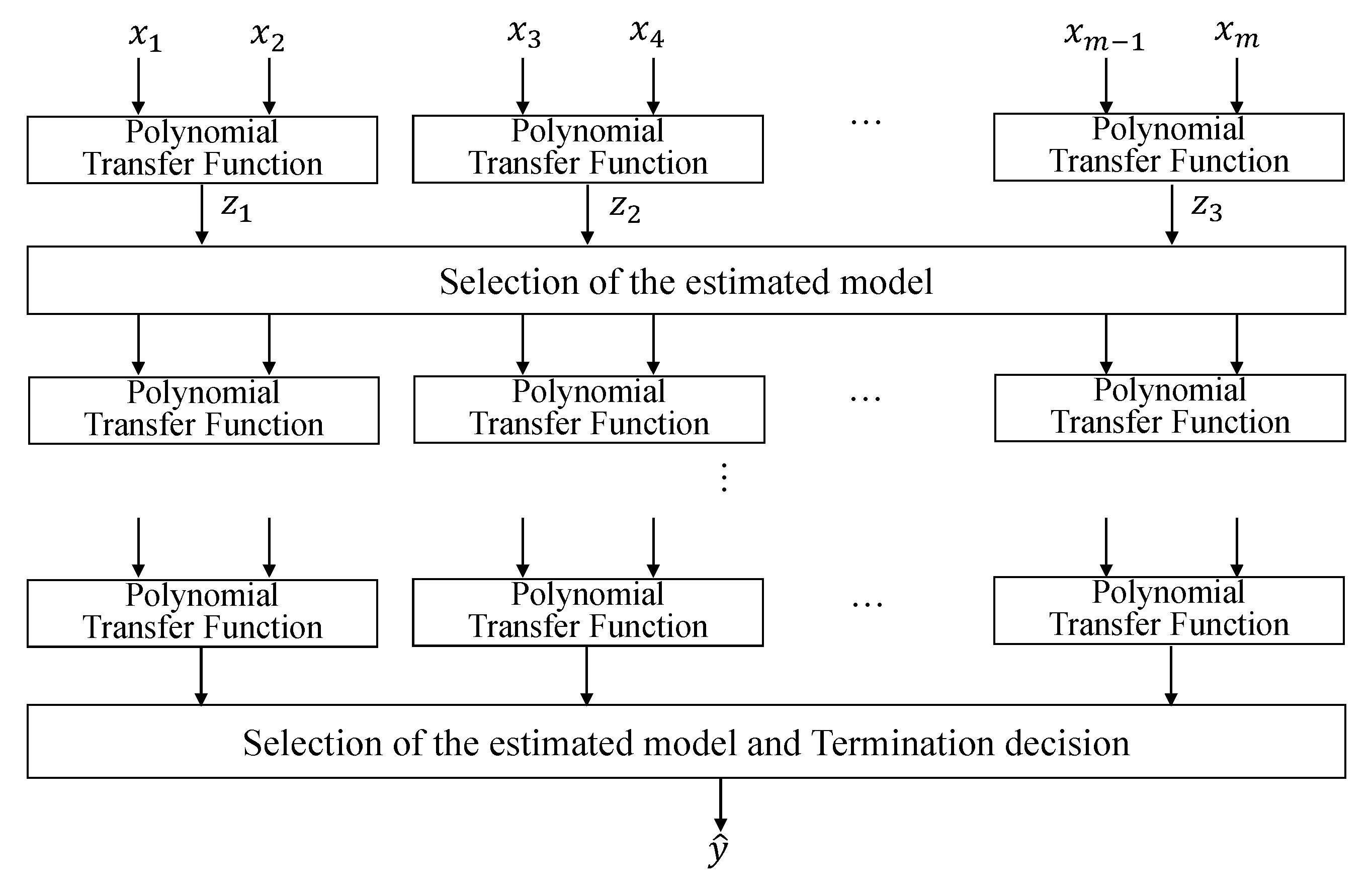
The main function of GMDH is based on the forward propagation of a signal through nodes of the net, similar to the principal used in classical neural nets, as shown in Figure 7 [25]. Every layer consists of simple nodes that each perform their own polynomial transfer function and pass their output to nodes in the next layer.

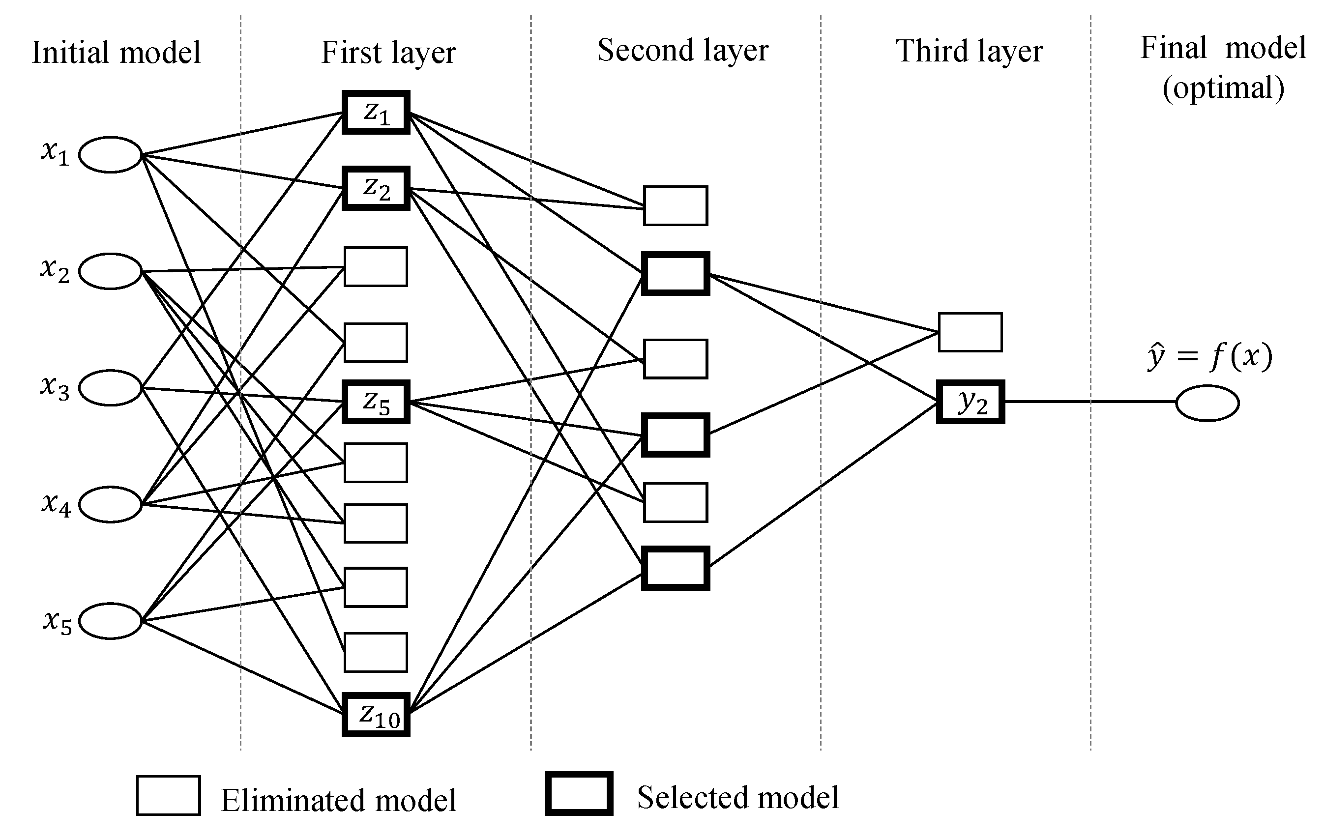
Figure 8 shows the diagram of the multilayered GMDH neural network model. The multilayer algorithm in a GMDH-type neural network builds a multilayer feed-forward neural network structure. Nodes in the hidden layers are developed for each layer that represents functions of every possible combination of two inputs to that layer. The combination of these terms that gives the lowest root mean square (RMS) error is kept as the transfer function of the neuron. By utilizing the external criterion, such as the lowest RMS error, the surviving neurons are then passed on to a new layer of the network. This continues to choose only optimal model (neuron) that supplies the best possible RMS error, or the network has reached a designer defined layer limit [24]. The basic steps involved in GMDH modeling are as follows [26]:

Step 1. Select input variables X = {$x_1$, $x_2$,…, $x_m$}. Divide the available data into training and checking data sets. Before applying the algorithm, the inputs and output are normalized.

• Inputs (candidates) are chosen as follows:
  • $x_1$: $a$-axis current, $i_a$ [$A$]
  • $x_2$: $b$-axis current, $i_b$ [$A$]
  • $x_3$: $c$-axis current, $i_c$ [$A$]
  • $x_4$: $\gamma$-axis current, $i_{\gamma }$ [$A$]
  • $x_5$: $\delta$-axis current, $i_{\delta }$ [$A$]
  • $x_6$: $\gamma$-axis voltage reference in synchronous reference frame, $v_{\gamma }$ [$V$]
  • $x_7$: $\delta$-axis voltage reference in synchronous reference frame, $v_{\delta }$ [$V$]
  • $x_8$: $\gamma$-axis voltage reference in stationary reference frame, $v_{\alpha }$ [$V$]
  • $x_9$: $\delta$-axis voltage reference in stationary reference frame, $v_{\beta }$ [$V$]
• Outputs (estimated models) are defined as follows:
  • ${\widehat{y}}_1$: $q$-axis inductance, $L_q$ [$H$]
  • ${\widehat{y}}_2$: position error, ${\theta }_e$ [$rad$]

Step 2. Separate data into two sets called the “training data set” and the “checking data set.” Construct new variables $Z=\left\{z_1,z_1,\dots ,z_m\right\}$ in the training data set and construct the regression polynomial for the first layer by forming the quadratic expression that approximates the output y.

Step 3. Identify the contributing nodes at each hidden layer according to the value of the root mean square (RMS) error. Eliminate the least effective variable by replacing the columns of X (old data) by the new columns of Z.

Step 4. The GMDH algorithm is carried out by repeating Steps 2 and 3 of the algorithm. When the errors of the checking data in each layer stop decreasing, the iterative computation is terminated.

The next step is to evaluate the output of each polynomial using the data points in the checking data. The output of each polynomial can be calculated using $\left(9\right).$

4.2. Sensorless Control Method with the Proposed Inductance Estimation Method

For data-driven approach-based parameter estimation, the sensorless controller was designed to estimate the inductance using a PNN algorithm and to follow the actual system output reference value. PNN design parameters were optimized to minimize RMS errors and deviations from the reference values. Considering the computational speed of the processor, the number of GMDH multilayers was set to ≤ 5. To cope with various load patterns, sufficient learning was performed on transient inputs, such as periodic functions of sine, step, and nonperiodic random functions. In addition, to prevent misoperation or decrease in accuracy of sensorless control because of inaccurate estimation of the parameter or unexpected problems, we configured the controller to perform additional monitoring and error detection by estimating the value of position error in real time.

Table 1. Polynomial neural network (PNN)-based training results.

No.	Input Variables for Training	$\mathit{q}$-$\mathbf{axis} \mathbf{Inductance}, {\mathit{L}}_{\mathit{q}}$		$\mathbf{Position} \mathbf{Error}, {\mathit{\theta }}_{\mathit{e}}$
		RMS Error (%)	R	RMS Error (rad)	R
Case 1	$i_{\delta }$, $v_{\gamma }$, $v_{\delta }$	0.61	0.9976	-	-
Case 2	$i_{\gamma }$, $i_{\delta }$, $v_{\gamma }$,$v_{\delta }$	0.57	0.9979	0.01242	0.8554
Case 3	$i_a$,$i_b$,$i_c$,$v_{\gamma }$,$v_{\delta }$	1.89	0.98713	0.01352	0.86149
Case 4	$i_a$,$i_b$,$i_c$,$v_{\alpha }$,$v_{\beta }$	1.98	0.9753	0.01812	0.7406

shows a comparison of RMS error and the linear regression performance index ($R$) of $q$-axis inductance ($L_q$) and position error (${\theta }_e$), which were estimated by PNN-based learning for each combination of input variables using MATLAB. In Table 1, $i_a$, $i_b$, $i_c$, $v_{\alpha }$, and $v_{\beta }$ are the $a,b,c$-phase current and stator voltage in the $\alpha$-$\beta$ stationary reference frame. The lowest RMS error was found in Case 2, applying four neurons of the current $i_{\gamma \delta }$ and voltage $v_{\gamma \delta }$ in the $\gamma$-$\delta$ reference frame as input parameters. However, both $v_{\gamma \delta }$ and $i_{\gamma \delta }$ were calculated in the $\gamma$-$\delta$ estimated synchronous reference frame and learning proceeded with these terms as input variables. As the estimated position error of the sensorless main controller increased, the accuracy of parameter estimation can also be reduced. In Case 4, $\alpha$-$\beta$ voltage in the stationary reference frame was used as input variables and the estimation error of $q$-axis inductance was relatively small. However, the position error was represented by the training result, which had a large RMS error and low linear regression performance. On the other hand, in Case 3, three-phase currents and $\gamma$-$\delta$ voltage in the synchronous frame were used as input variables. Although $q$-axis inductance and position error were slightly larger than in Case 2, the effect of the $\gamma$-$\delta$ current from the rotor position error could be minimized by using the three-phase currents directly measured in the current sensors. Therefore, the regression and training for $q$-axis inductance and position error were carried out in Case 3.

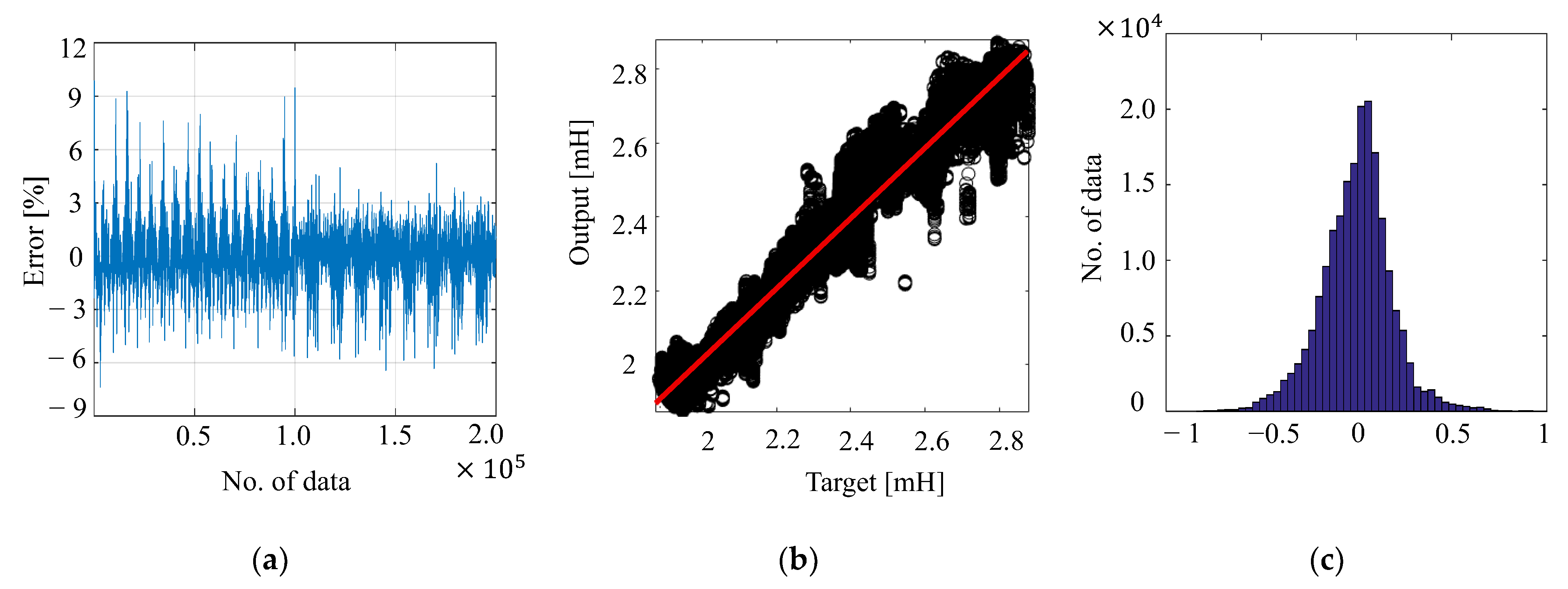
Figure 9 represents $q$-axis inductance estimation error, a linear regression plot, and error histogram of the PNN-based machine learning simulation with five input variables selected in Case 3. The analysis results indicated sufficiently low RMS error (<2%) and high linearity, R > 0.95. In Figure 9b,c, characteristics of estimation error are identified.

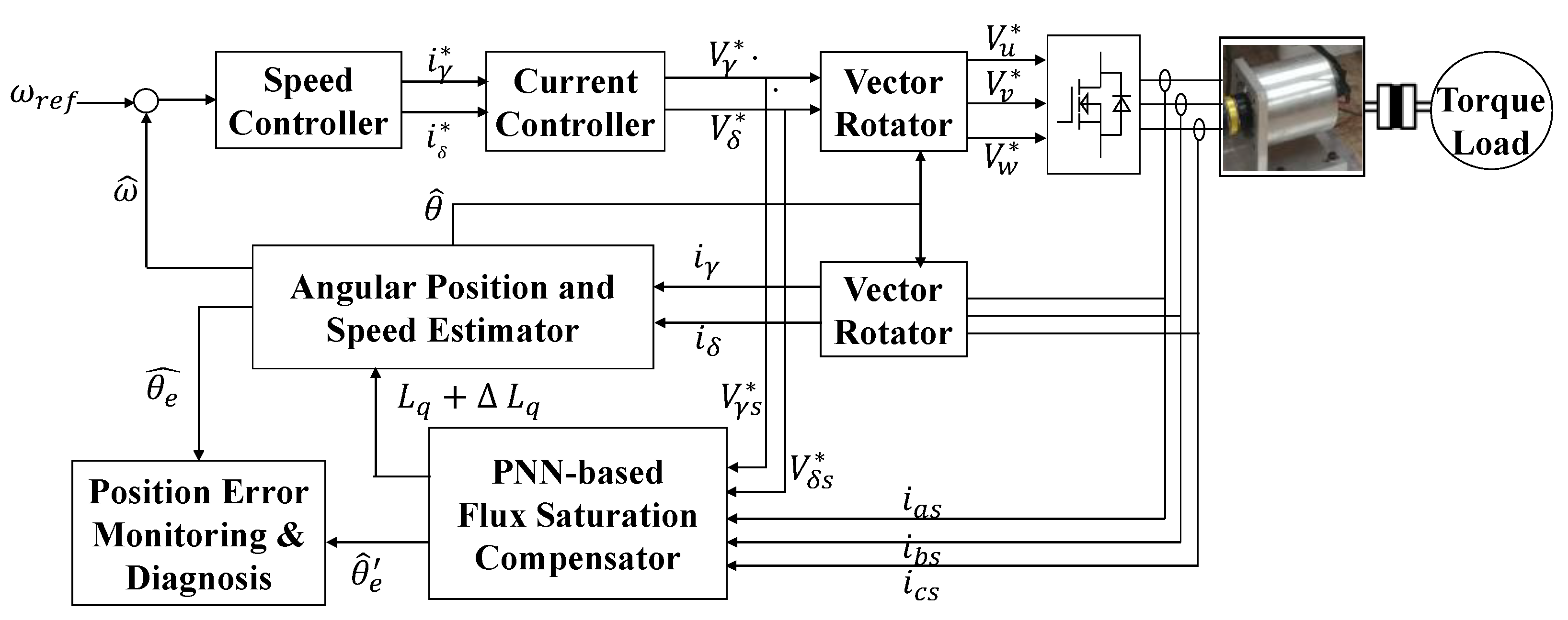
Figure 10 shows a block diagram of the entire PMSM sensorless control system with the proposed inductance estimation based on the PNN machine learning algorithm. The PNN algorithm is used to derive a polynomial expression-based numerical model of the inductance parameters through machine learning from multiple variable inputs, such as the measured current and voltage reference. The inductance values that are estimated through machine learning are fed back to the sensorless controller again and compensate the magnetic fluctuation in real-time to reduce speed ripple. Comparing the position error ${\theta }_e$ and ${\theta }_e^{\prime }$ from the sensorless position estimator and the PNN algorithm, one can perform position estimation error monitoring and diagnosis. If the difference between these values or an abnormal operation is detected, an error flag is transmitted to the sensorless main controller. In addition, the gain factor of the PNN is adjusted to limit the magnetic saturation compensation or to stop the system by gradually reducing its operating speed.

5. Simulation and Experimental Results

5.1. Simulation Results

A software simulation was performed for an entire sensorless system to validate the proposed PNN-based compensation method and to confirm results from position estimation error and speed ripple. The parameters of the PMSM used in the simulations were the same as the motors used in the practical experiments, as shown in

Table 2. Motor parameters.

Parameter	p-Value	Unit
Rated power	3	kW
Rated current	20	A
Winding resistance	0.3	$\mathsf{\Omega }$
Number of poles	6	-
Number of slots	27	-
$d$-axis inductance	1.5	mH
$q$-axis inductance	2.0	mH

.

The sensorless PMSM drive has a periodic load torque from the compression/charging and exhaust/discharging stroke in the compressor and pump. If the periodic load torque is not compensated by the PMSM torque, it invokes speed ripple, noise, and vibration. Especially at a low speed, when vibration occurs, there is mechanical fatigue failure. The periodic load torque can be compensated by applying a load torque compensator. However, magnetic saturation occurs due to increasing compensation current, which degrades the accuracy of sensorless speed control and the load torque compensator.

First, it is assumed that the periodic load torque is fully known and the $\delta$-axis compensation current depending on the load is expressed as the sum of the first frequency component, $I_S$, with constant amplitude and DC offset $I_{DC}$:

$$i_{\delta }=I_{S}sin\omega t+I_{DC}$$

(11)

where $i_{\delta }$ is $\delta$-axis compensation current, and $\omega$ is first frequency component of rotor speed.

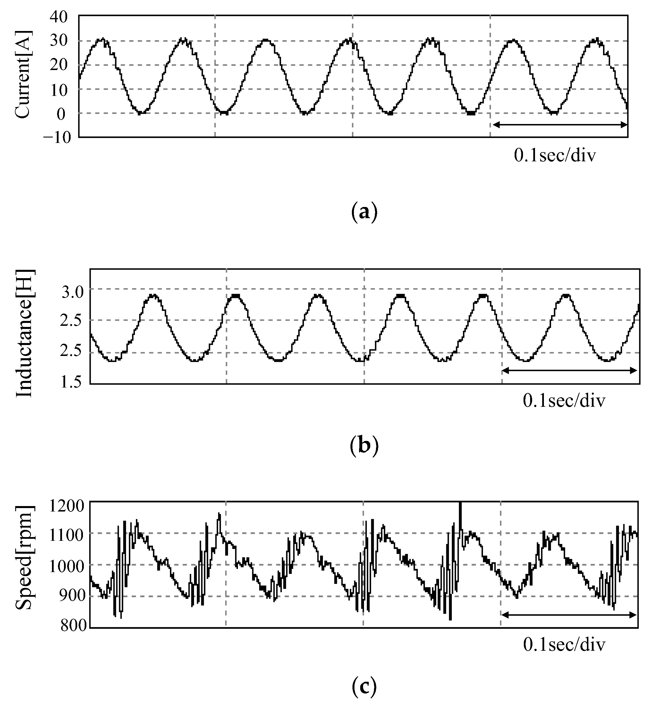
The $\gamma$-axis compensation current is obtained from the $\delta$-axis compensation current on the basis of the rule of maximum torque per ampere. If the rotor position is correctly estimated, even with varying inductance, the periodic load torque would be fully compensated with (11). In the simulation, both the DC offset and the magnitude of the first frequency component of the current were applied as 15 A: $I_S=I_{DC}=15 A$. Figure 11 shows the simulation plots of inductance and speed ripple generated by the load torque compensation current during constant speed operation at 1000 rpm (16.67 Hz) and without the inductance estimation. When the $\delta$-axis current was controlled by a maximum amplitude of 30 A, as shown in Figure 11a, the actual inductance changed, as shown in Figure 11b. When the control was performed without compensating the inductance variations caused by magnetic saturation, a high ripple of the estimated speed occurred, as shown in Figure 11c.

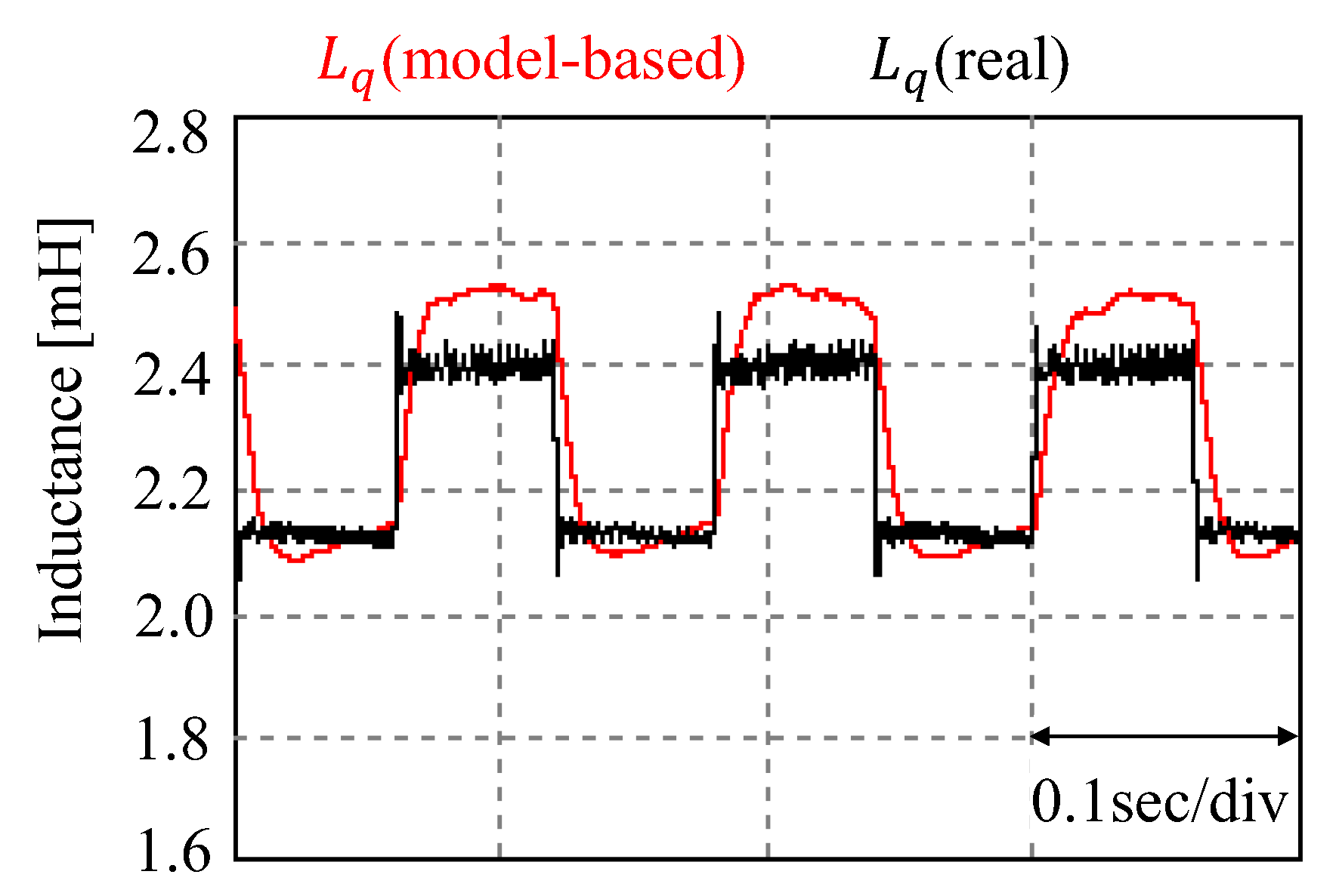
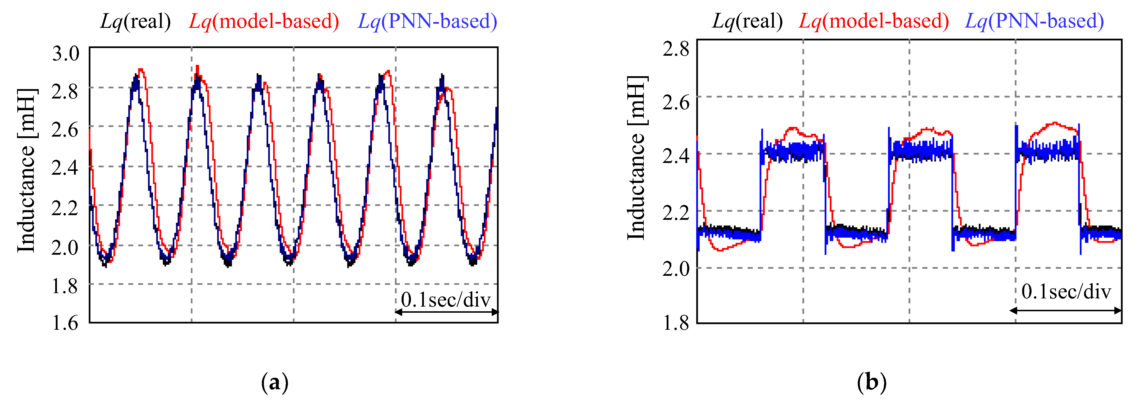
Figure 12 presents comparison plots of the estimated inductance values obtained from the mathematical model-based method and the PNN-based machine learning method under a periodic load torque. For the inductance estimated by the mathematical model-based method, DC offset and time delay occurred. On the other hand, in the case of the PNN-based learning method, good correspondence was observed between the estimated values and the real values. The rotor position error, $\Delta {\widehat{\theta }}_e$, and extended EMF error, $\Delta {\hat{e}}_{\mathsf{\gamma }},$ could be easily obtained by applying the inductance variation $\Delta L_q$, derived in the form of a quadratic polynomial equation through machine learning into (3) and (4). In addition, through the low-pass filter and integrator in Figure 2, the estimated speed ripple, $\Delta {\widehat{\omega }}_o$, due to magnetic saturation, could be obtained.

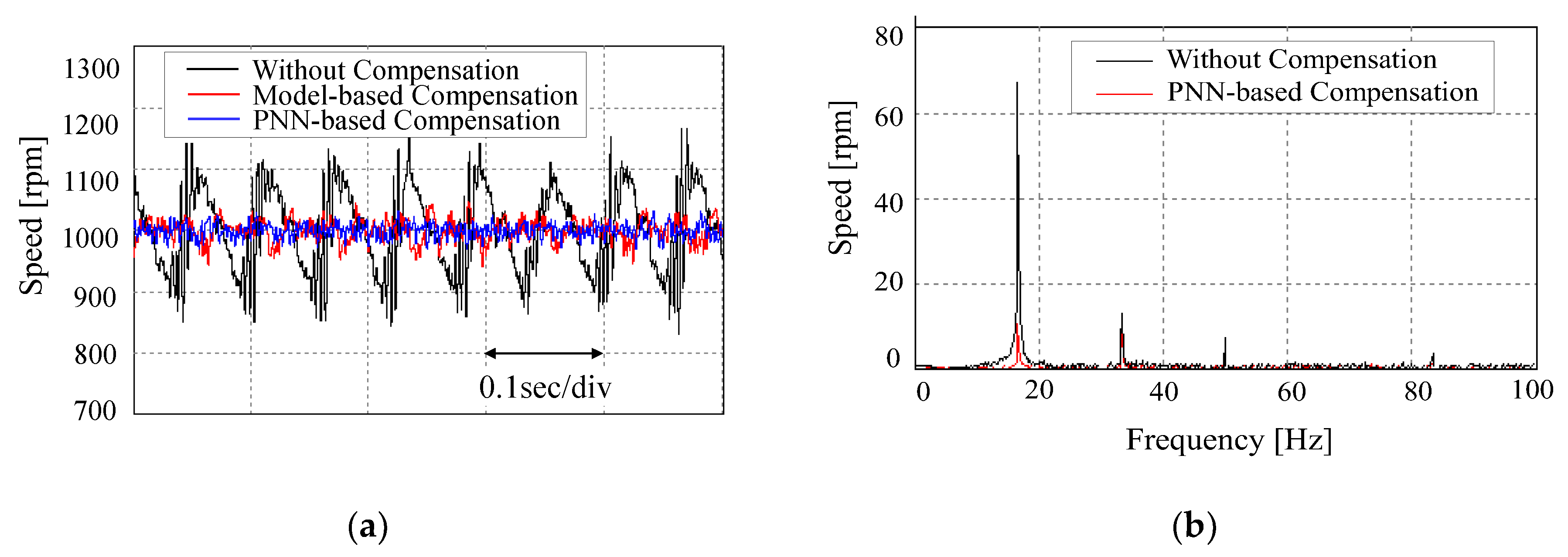
As shown in Figure 13, the estimated speed without compensation was compared with the two estimated speeds with feedback compensation for inductance variation on the basis of the model-based method and PNN-based method under the condition of constant speed (1000 rpm). In the uncompensated condition, the ripple of speed error was about ±15%, as shown in Figure 13a. On the other hand, when the model-based compensation was applied, the ripple was reduced to less than ±5%, and when the PNN-based compensation was applied, it was reduced to approximately ±3%. In addition, as a comparison result in the frequency domain, the magnitude of the first to third order harmonic of the fundamental frequency (16.67 Hz) was high before applying compensation control, as shown in Figure 13b. However, after applying compensation control, it can be seen that the magnitude was significantly decreased compared to the uncompensated condition. In particular, the magnitude of the fundamental frequency was reduced by approximately 85%.

5.2. Experimental Results

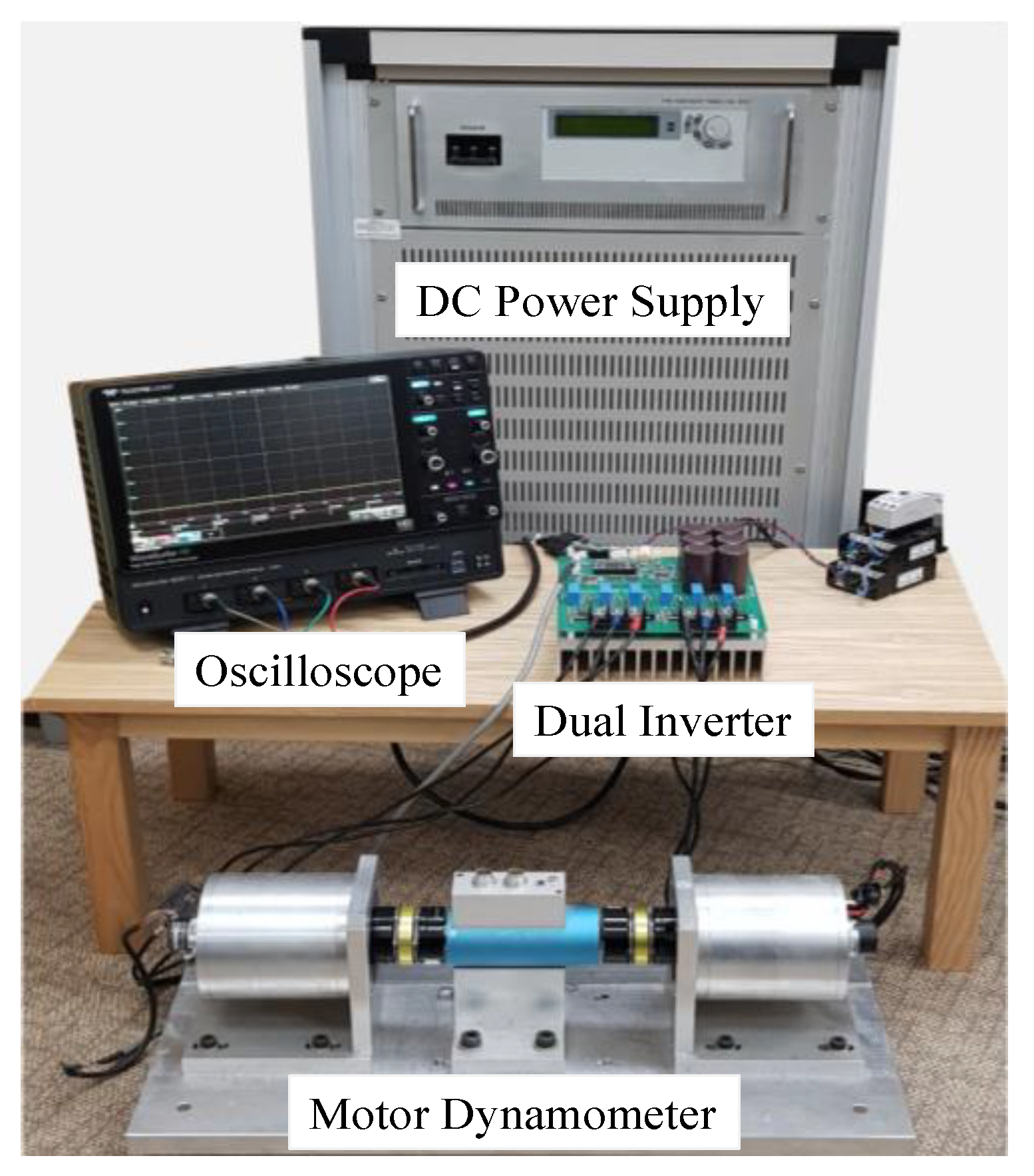
Figure 14 shows the experimental configuration used in this study. Two hybrid vehicle compressors were disassembled and manufactured as a test motor and a load motor. To control each motor, we designed and implemented a dual inverter.

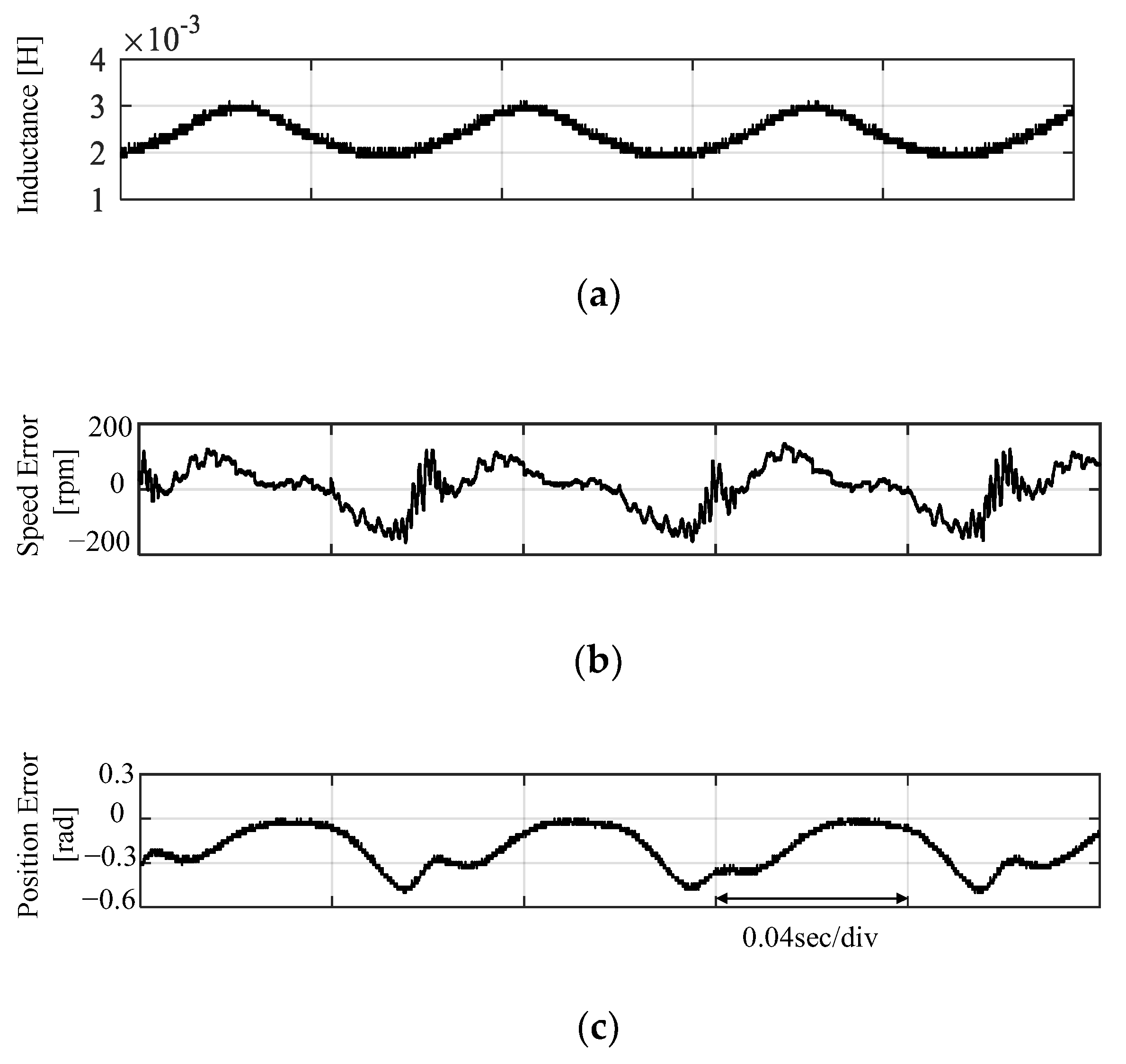
Figure 15a shows the $q$-axis inductance with magnetic saturation when $\delta$-axis current was controlled by a maximum amplitude of 30 A periodic signal during constant speed operation at 1000 rpm. These conditions are the same as the simulation load conditions. Figure 15b,c shows the speed error and the position error when controlling without compensation of the inductance variation. In the experimental results, since the $q$-axis inductance was controlled by a constant value under the uncompensated condition, the amplitude of the speed error and position error were up to 15% due to magnetic saturation.

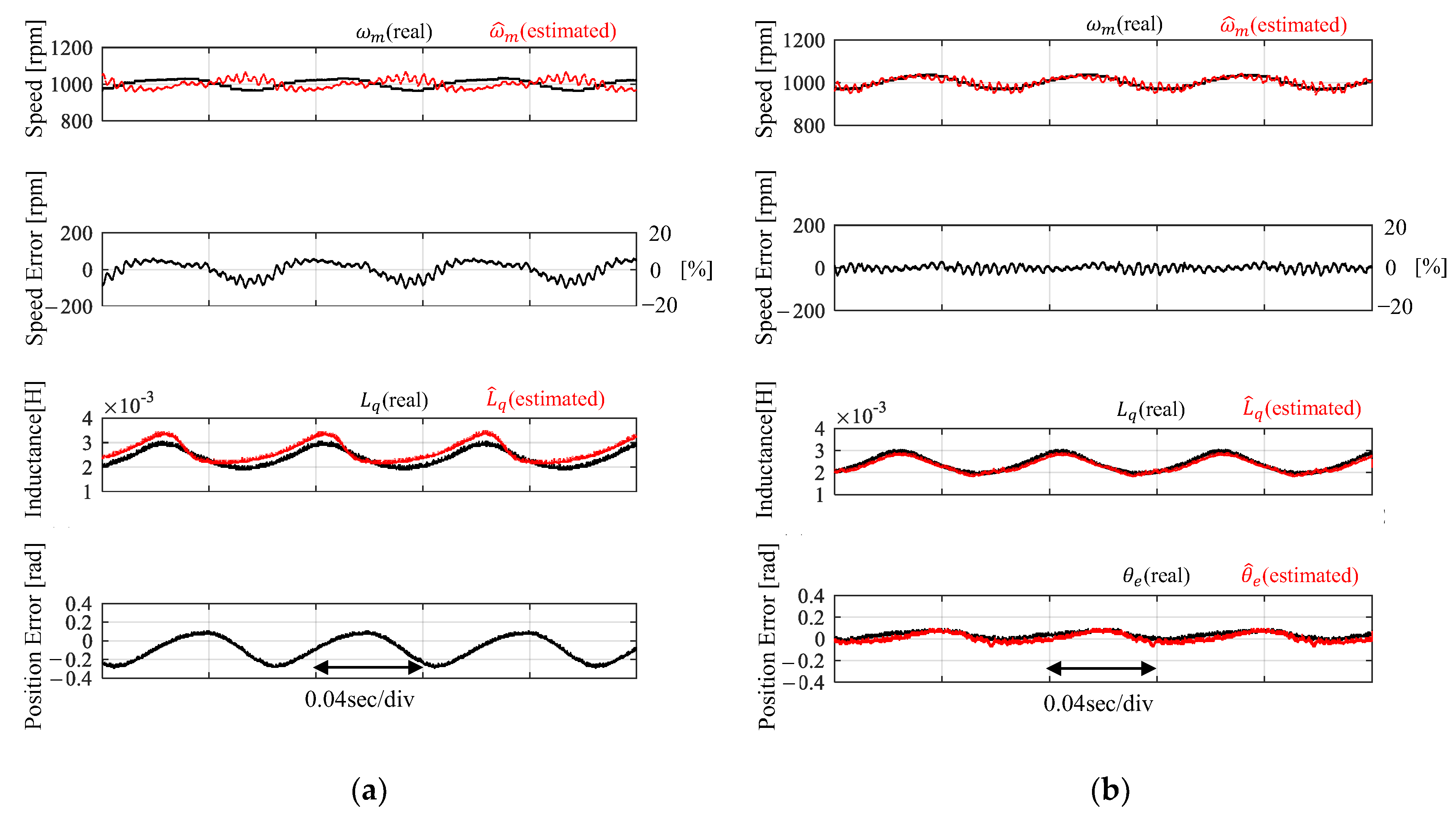
Figure 16 shows a comparison of the experiment result with the model-based $q$-axis inductance compensation method and with PNN-based compensation. When the model-based compensation method was applied, the estimated $q$-axis inductance had a time delay and some distortion compared to the actual inductance. On the other hand, the inductance estimated by the PNN-based machine learning method almost tracked the actual value completely. Therefore, it was confirmed that the ripple of the speed error was improved by 3–4% when compensation control was performed on the basis of the PNN algorithm and compared with the model-based compensation method. However, despite performing calibration controls, the speed ripple of the experimental results was higher than that of the simulation because of system vibration due to mechanical alignment problems and electrical imbalance, which were not reflected in the simulation.

In addition, it could be confirmed that the estimated position error based on the PNN algorithm was properly monitored in real time to appropriately respond to fault conditions, such as large error in the estimated value or unstable system control.

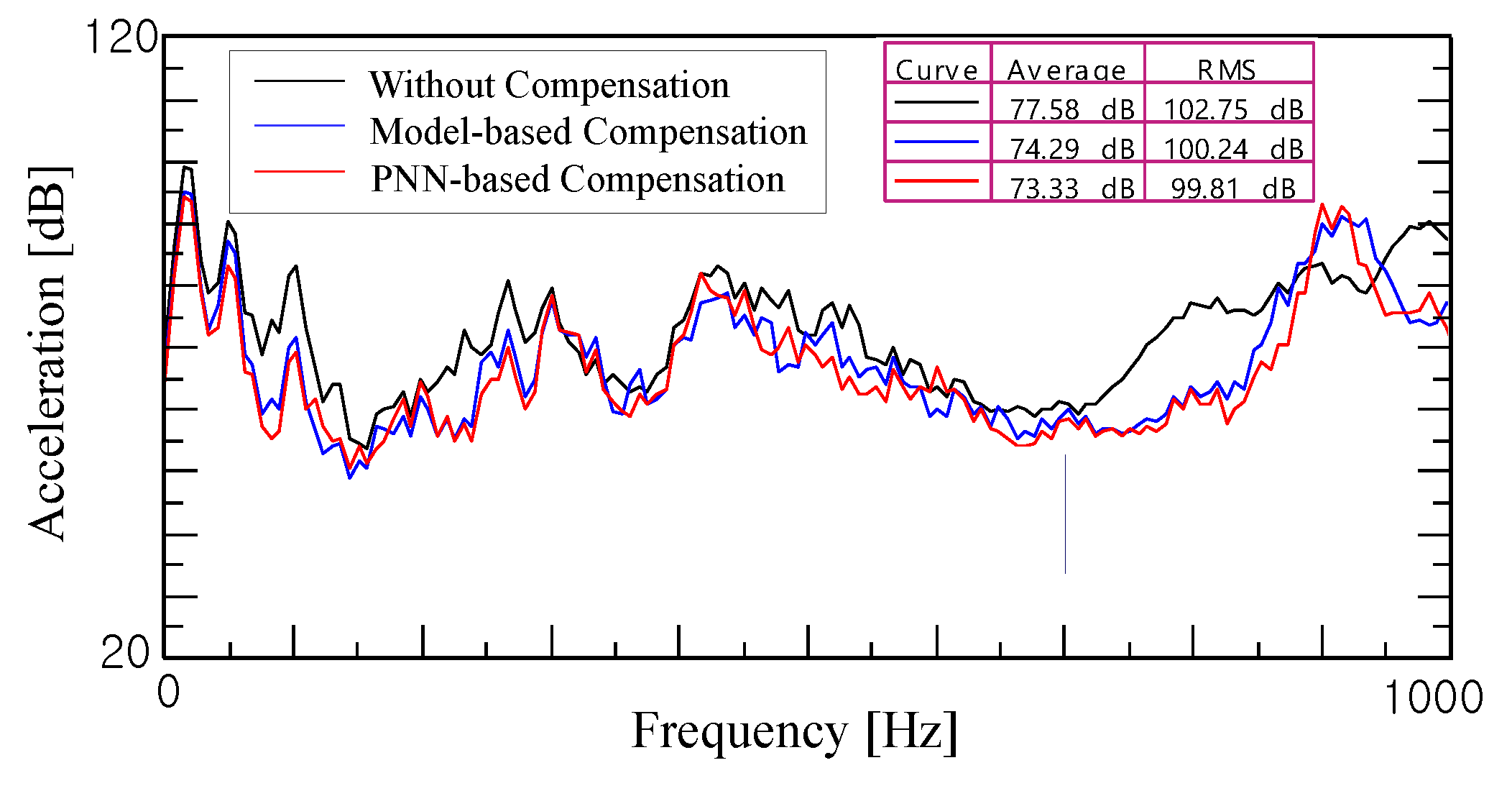
To evaluate the dynamic NVH performance of motors for the compressor, we mounted acceleration sensors on the motor housing, and real-time data were collected. In addition, vibration data with or without compensation control under magnetic saturation conditions were compared and analyzed. Figure 17 shows comparison results of the vibration magnitude without compensation and with feedback compensation based on the model-based method and PNN-based method at a speed of 16.67 Hz (1000 rpm). For the condition without compensation, the vibration magnitude was 77.58 dB in terms of the average value. In the case of model-based compensation and PNN-based compensation, the average values of vibration were 74.29 dB and 73.33 dB, respectively. Therefore, it was confirmed that the vibration magnitude of PNN-based compensation was the lowest in both average value and RMS value, and approximately 4 dB smaller than the uncompensated condition.

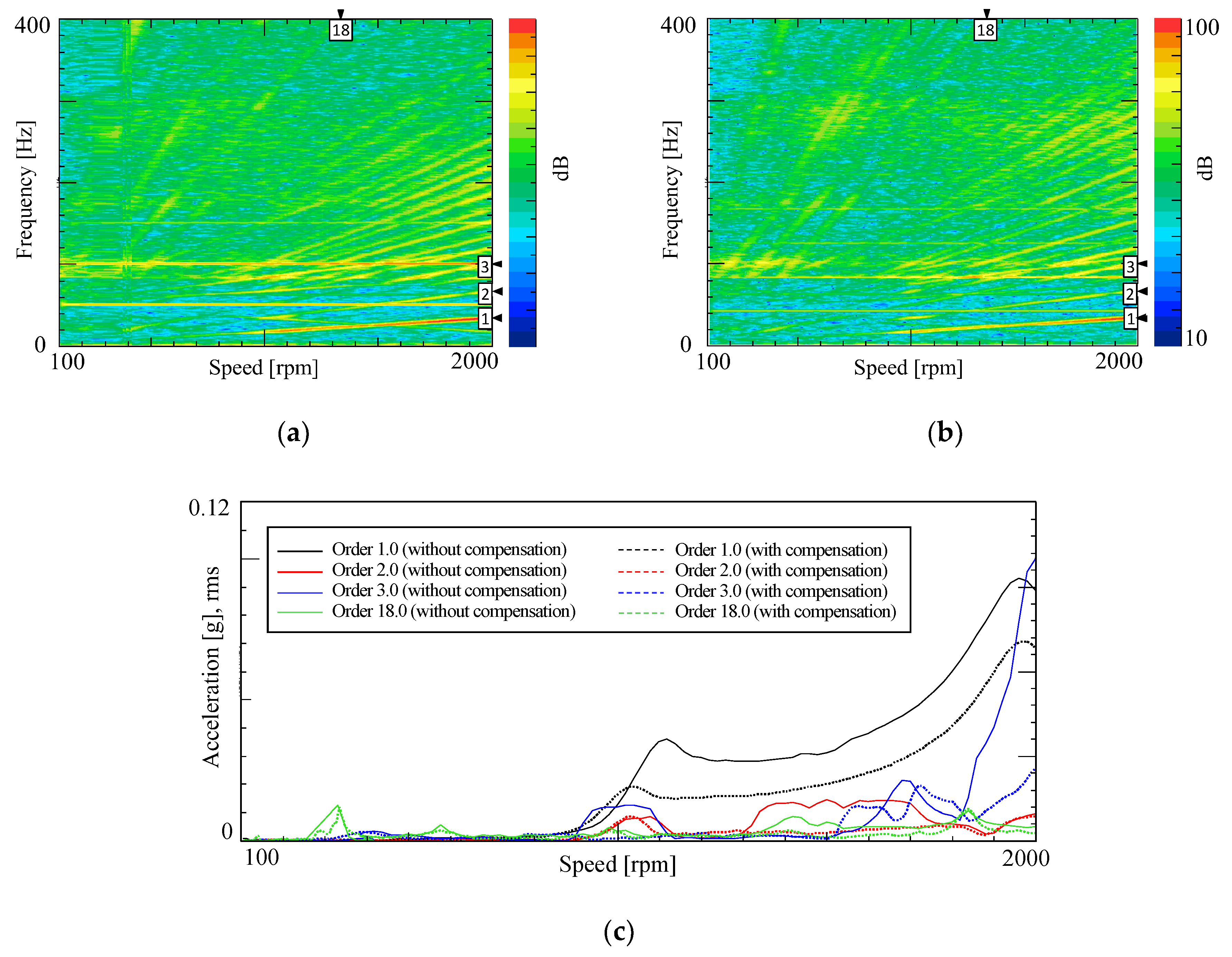
The vibration measurement results without compensation were compared to that with PNN-based compensation using a color map and order tracking analysis in speed sweeps from 0 to 2000 rpm under a periodic load torque, as shown in Figure 18. From the order analysis results, we confirmed that the first order component, which is the fundamental frequency component of the rotational speed, was dominant to the vibration and magnitude of the vibration after compensation was significantly reduced from 0.095 g to 0.070 g on the basis of the maximum value. Moreover, the vibration magnitude was reduced in the second and third harmonics of the fundamental frequency component. The vibration of the 18th order component, which is the cogging torque frequency due to the number of poles and slots, was also improved. Therefore, it was recognized that the vibration reduction effect of compensation control was relatively high in the low frequency region since the first order component, which coincided with the load torque frequency, acted as the main excitation source and caused vibration. In addition, it was determined that the mechanical vibration component of the rotation frequency due to the influence of mechanical alignment, runout, and unbalance still remained.

6. Conclusions

This paper analyzed the position and speed estimation error of a PMSM sensorless drive caused by magnetic saturation. To compensate magnetic saturation, we proposed a $q$-axis inductance estimation method with PNN machine learning. The learning model, based on the PNN-based GMDH algorithm, was configured to correspond with a nonlinear sensorless control system. Moreover, to effectively respond to fault situations, such as an unknown disturbance or increased errors in the position error in the sensorless method, we also estimated the position error and monitored it in real-time.

For each case of applying a compensator on the basis of the mathematical observer model and the proposed PNN machine learning model, we compared and analyzed the control performances through simulation and experiment. The experimental results indicated that the model-based compensator had problems, including time delay and DC offset, and estimation accuracy was further decreased when a dynamic transient load was applied. However, in the case of the PNN-based compensator, the compensation control performance was accurate and fast.

Through simulation and experimental results, we confirmed that the proposed compensation method can be applied to obtain real-time estimation performance for parameters that are relatively simple and accurate. In addition, by applying the proposed method to a nonlinear sensorless system, we verified a more efficient improvement of the control performance compared to the conventional method. Moreover, through a vibration test for each speed/frequency, we confirmed that the sensorless control system with the proposed compensation method showed clear NVH improvement in low-frequency regions, having a large fluctuation of parameters compared with the uncompensated system. Because the PNN-based estimator is adaptable to various operating conditions and is simple in design, it can be applied to various types of motors for parameter estimation and compensation by performing simple training with appropriate load models.

References

- Tang, P.; Dai, Y.; Li, Z. Unified Predictive Current Control of PMSMs with Parameter Uncertainty. Electronics 2019, 8, 1534. [Google Scholar] [CrossRef] [Green Version]
- Morimoto, S.; Kawamoto, K.; Sanada, M.; Takeda, Y. Sensorless control strategy for salient-pole PMSM based on extended EMF in rotating reference frame. IEEE Trans. Ind. Appl. 2002, 38, 1054–1061. [Google Scholar] [CrossRef]
- Mizutani, R.; Takeshita, T.; Matsui, N. Current model-based sensorless drives of salient-pole PMSM at low speed and standstill. IEEE Trans. Ind. Appl. 1998, 34, 841–846. [Google Scholar] [CrossRef]
- Zhu, Y.; Tao, B.; Xiao, M.; Yang, G.; Zhang, X.; Lu, K. Luenberger Position Observer Based on Deadbeat-Current Predictive Control for Sensorless PMSM. Electronics 2020, 9, 1325. [Google Scholar] [CrossRef]
- Hoai, H.-K.; Chen, S.-C.; Chang, C.-F. Realization of the Neural Fuzzy Controller for the Sensorless PMSM Drive Control System. Electronics 2020, 9, 1371. [Google Scholar] [CrossRef]
- Imaeda, Y.; Doki, S.; Hasegawa, M.; Matsui, K.; Tomita, M.; Ohnuma, T. PMSM position sensorless control with extended flux observer. In Proceedings of the 37th Annual Conference of the IEEE Industrial Electronics (IECON 2011), Melbourne, Australia, 7–10 November 2011; pp. 4721–4726. [Google Scholar]
- Cho, K.Y. Sensorless control for a PM synchronous motor in a single piston rotary compressor. J. Power Electron. 2006, 6, 29–37. [Google Scholar]
- Young, C.M.; Liu, C.C.; Liu, C.H. Vibration analysis of rolling piston-type compressors driven by single-phase induction motor. In Proceedings of the 19th Annual Conference of IEEE Industrial Electronics (IECON ’93), Maui, HI, USA, 15–19 November 1993; pp. 918–923. [Google Scholar]
- Lee, K.W.; Ha, J.I. Evaluation of back-EMF estimators for sensorless control of permanent magnet synchronous motors. J. Power Electron. 2012, 12, 604–614. [Google Scholar] [CrossRef]
- Ichikawa, S.; Tomita, M.; Doki, S.; Okuma, S. Sensorless control of permanent-magnet synchronous motors using online parameter identification based on system identification theory. IEEE Trans. Ind. Electr. 2006, 53, 363–371. [Google Scholar] [CrossRef]
- Morimoto, S.; Sanada, M.; Takeda, Y. Effect and Compensation of Magnetic Saturation in Flux-Weakening Controlled Permanent Magnet Synchronous Motor Drives. IEEE Trans. Ind. Appl. 1994, 30, 1632–1637. [Google Scholar] [CrossRef]
- Ichikawa, S.; Tomita, M.; Doki, S.; Okuma, S. Sensorless Control of Synchronous Reluctance Motors Based on Extended EMF Models Considering Magnetic Saturation with Online Parameter Identification. IEEE Trans. Ind. Appl. 2006, 30, 1264–1274. [Google Scholar] [CrossRef]
- Underwood, S.J.; Husain, I. Online Parameter Estimation and Adaptive Control of Permanent-Magnet Synchronous Machines. IEEE Trans. Ind. Electr. 2010, 57, 2435–2443. [Google Scholar] [CrossRef]
- Lin, H.; Hwang, K.Y.; Kwon, B.I. An Improved Flux Observer for Sensorless Permanent Magnet Synchronous Motor Drives with Parameter Identification. J. Electr. Eng. Technol. 2013, 8, 516–523. [Google Scholar] [CrossRef] [Green Version]
- Wang, A.; Zhang, L.; Dong, S. Dynamic performance improvement based on a new parameter estimation method for IPMSM used for HEVs. In Proceedings of the 37th Annual Conference of the IEEE Industrial Electronics (IECON 2011), Melbourne, Australia, 7–10 November 2011; pp. 1825–1829. [Google Scholar]
- Hasegawa, M.; Matsui, K. Position sensorless control for interior permanent magnet synchronous motor using adaptive flux observer with inductance identification. IET Electr. Power Appl. 2009, 3, 209–217. [Google Scholar] [CrossRef]
- Kawamura, N.; Nomura, Y.; Zanma, T.; Liu, K.Z.; Hasegawa, M. Q-axis inductance identification for IPMSMs using DyCE principle based adaptive flux observer. In Proceedings of the 2020 International Symposium on Power Electronics, Electrical Drives, Automation and Motion (SPEEDAM), Sorrento, Italy, 24–26 June 2020; pp. 699–704. [Google Scholar]
- Fan, S.S.; Hsu, C.; Tsai, D.; He, F.; Cheng, C. Data-Driven Approach for Fault Detection and Identification in Semiconductor Manufacturing. IEEE Trans. Autom. Sci. Eng. 2020, 17, 1925–1936. [Google Scholar] [CrossRef]
- Farlow, S. The GMDH algorithm of Ivakhnenko. Am. Stat. 1981, 35, 210–215. [Google Scholar]
- Farlow, S. Self-Organizing Methods in Modeling: GMDH Type Algorithms; CRC Press: Boca Raton, FL, USA, 1984; pp. 8–86. [Google Scholar]
- Guo, H.; Sagawa, S.; Watanabe, T.; Ichinokura, O. Sensorless driving method of permanent-magnet synchronous motors based on neural networks. IEEE Trans. Magn. 2003, 39, 3247–3249. [Google Scholar]
- Elbuluk, M.; Liu, T.; Husain, I. Neural network-based model reference adaptive systems for high performance motor drives and motion controls. In Proceedings of the 2000 IEEE Industry Applications Conference, Thirty-Fifth IAS Annual Meeting and World Conference on Industrial Applications of Electrical Energy, Rome, Italy, 8–12 October 2000; pp. 959–965. [Google Scholar]
- Fan, S.S.; Chang, Y.; Aidara, N. Nonlinear Profile Monitoring of Reflow Process Data Based on the Sum of Sine Functions. Qual. Reliab. Eng. Inter. 2012, 29, 743–758. [Google Scholar] [CrossRef]
- Pandya, A.S.; Gilbar, T.; Kim, K.B. Neural Network Training Using a GMDH Type Algorithm. Int. J. Fuzzy Logic Intell. Syst. 2005, 5, 52–58. [Google Scholar] [CrossRef] [Green Version]
- Iwasaki, M.; Takei, H.; Matsui, N. GMDH-based modeling and feedforward compensation for nonlinear friction in table drive systems. IEEE Trans. Ind. Electr. 2003, 50, 1172–1178. [Google Scholar] [CrossRef]
- Kim, J.H.; Matsui, Y.; Hayakawa, S.; Suzuki, T.; Okuma, S.; Tsuchida, N. Acquisition and modeling of driving skills by using three dimensional driving simulator. IEICE Trans. Fundam. Electr. Comm. Comput. 2005, E88-A, 770–778. [Google Scholar] [CrossRef]
Figure 1.
Space vector diagram of a permanent magnet synchronous motor (PMSM).
Figure 2.
Block diagram of position estimator using extended electromotive force (EMF)-based sensorless control [2].
Figure 3.
Comparison of estimated rotor position errors (a) without and (b) with the voltage error of the - axes extended back EMF.
Figure 4.
Simulation results of and , where , and .
Figure 5.
Schematic illustrating the conventional compensation method for magnetic saturation.
Figure 6.
Step response simulation results of observer model-based inductance estimation.
Figure 7.
Self-organizing process for a GMDH algorithm regression model.
Figure 8.
Diagram of the multilayered GMDH neural network model.
Figure 9.
PNN-based machine learning and optimization results of -axis inductance (Case 3). (a) Plot of error between target and output; (b) scatterplot of linear regression; (c) error histogram.
Figure 10.
Block diagram of the sensorless control system with a PNN-based inductance estimation.
Figure 11.
Simulation results when the load fluctuated at 16.7 Hz for (a) -axis current, (b) -axis inductance, and (c) estimated speed.
Figure 12.
-axis inductance comparison of real, model-based, and PNN-based methods in (a) sine response and (b) step response.
Figure 13.
Comparison of estimated speed between no compensation, model-based compensation, and PNN-based compensation in the (a) time domain and (b) frequency domain (FFT).
Figure 14.
Experimental configuration.
Figure 15.
Plots when the motor operated at 16.7 Hz without compensation for (a) -axis inductance, (b) speed error, and (c) position error.
Figure 16.
Plots of speed, speed error, inductance, and position error when the motor operated at 16.7 Hz with the (a) model-based method and (b) PNN-based compensation method.
Figure 17.
Frequency analysis of vibration measurement results (dB reference level = 1 × 10⁻⁶ [g]).
Figure 18.
Vibration order analysis based on a (a) colormap without compensation, (b) colormap with compensation, and (c) order tracking results.