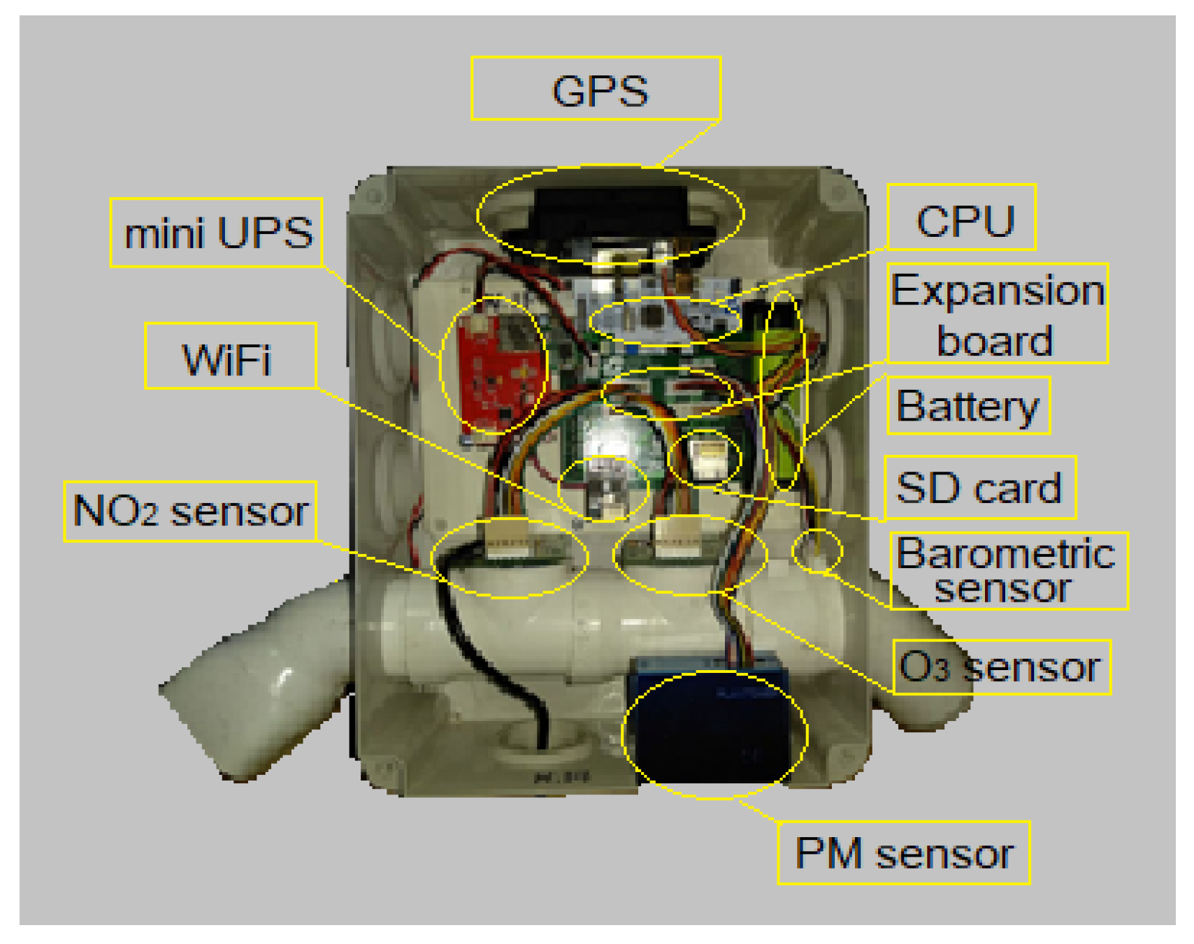
Figure 1.
Wireless connectivity (Wi-Fi).
Figure 1.
Wireless connectivity (Wi-Fi).
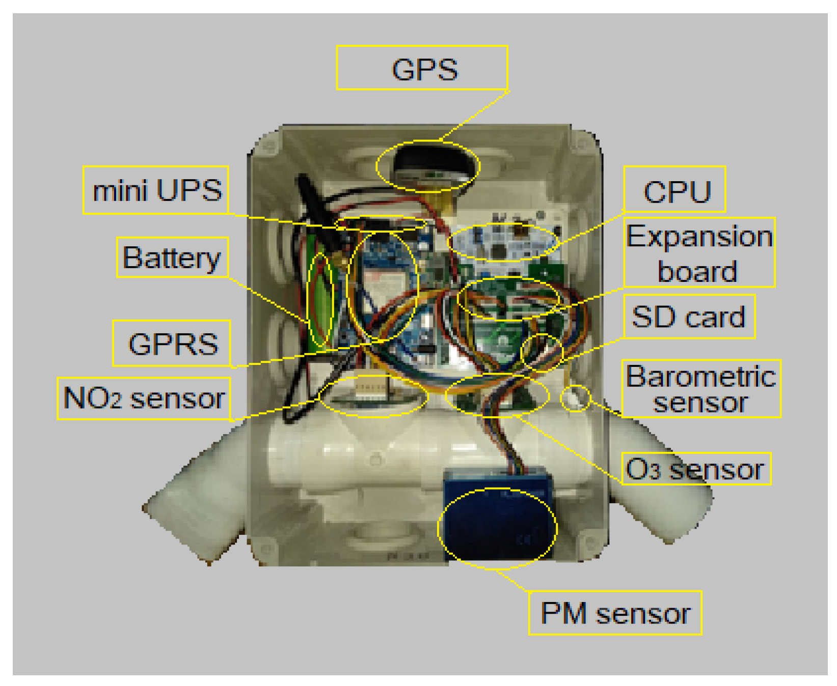
Figure 2.
Mobile network connectivity (GPRS).
Figure 2.
Mobile network connectivity (GPRS).
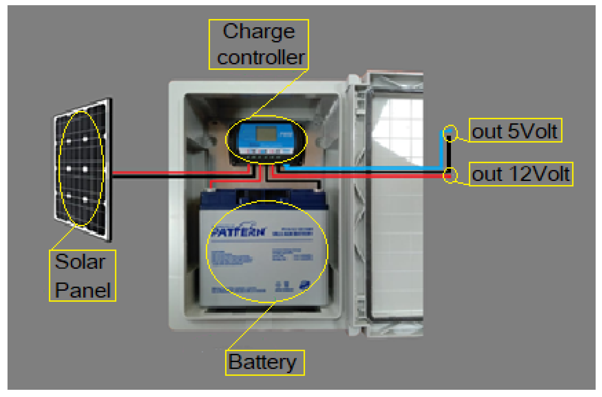
Figure 3.
Autonomous power supply.
Figure 3.
Autonomous power supply.
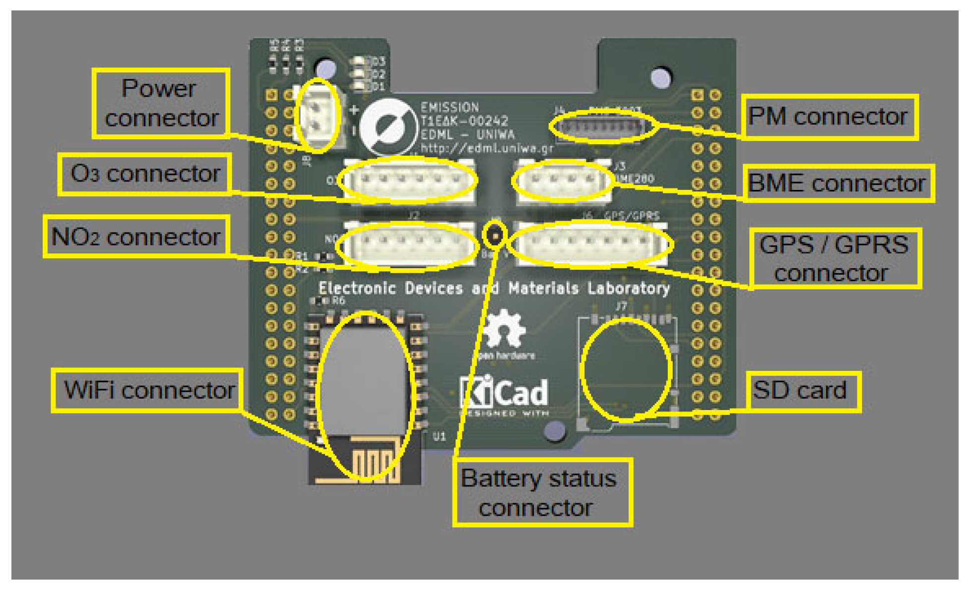
Figure 4.
Expansion board.
Figure 4.
Expansion board.
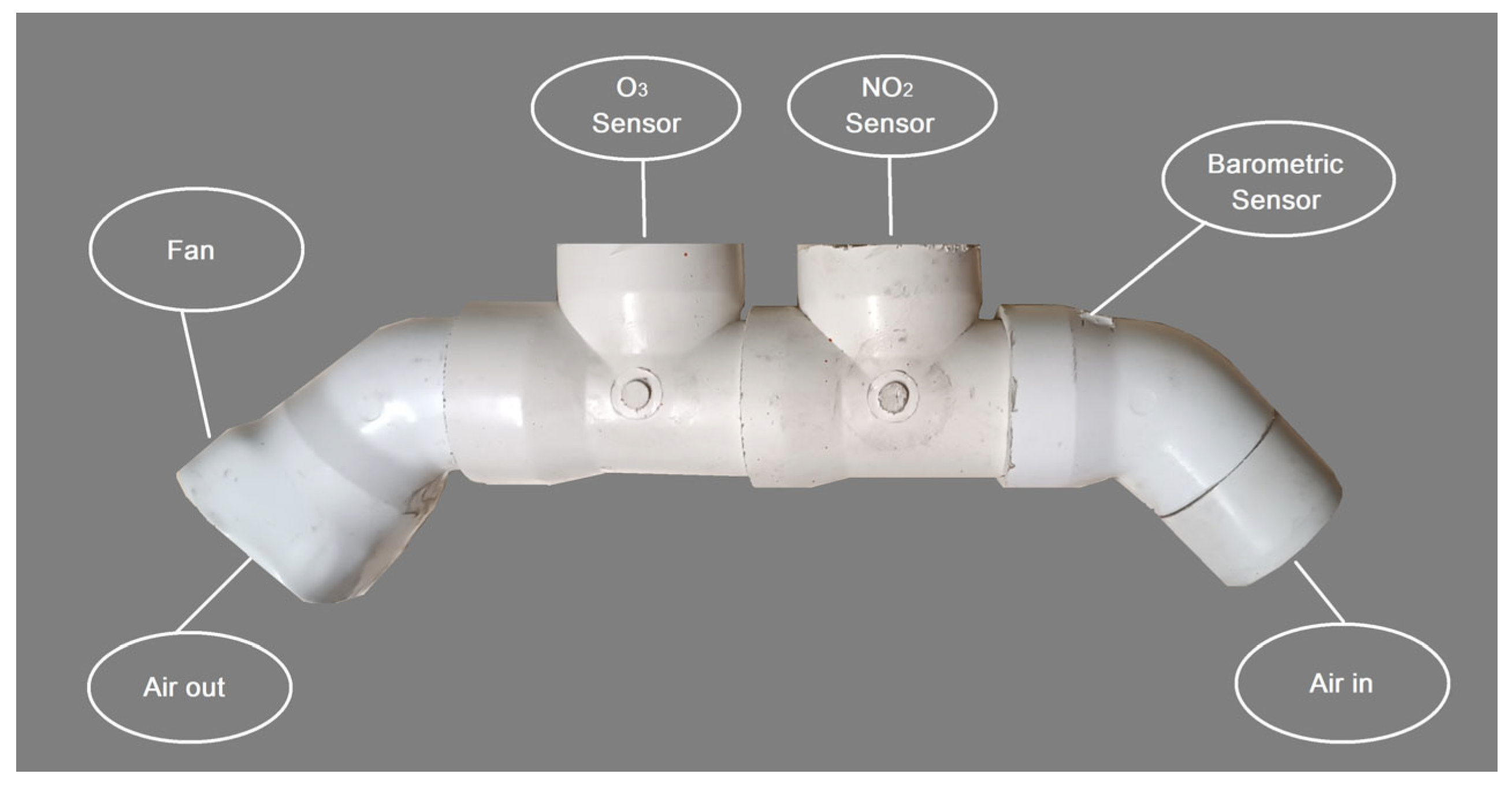
Figure 5.
Sensor holder tube.
Figure 5.
Sensor holder tube.
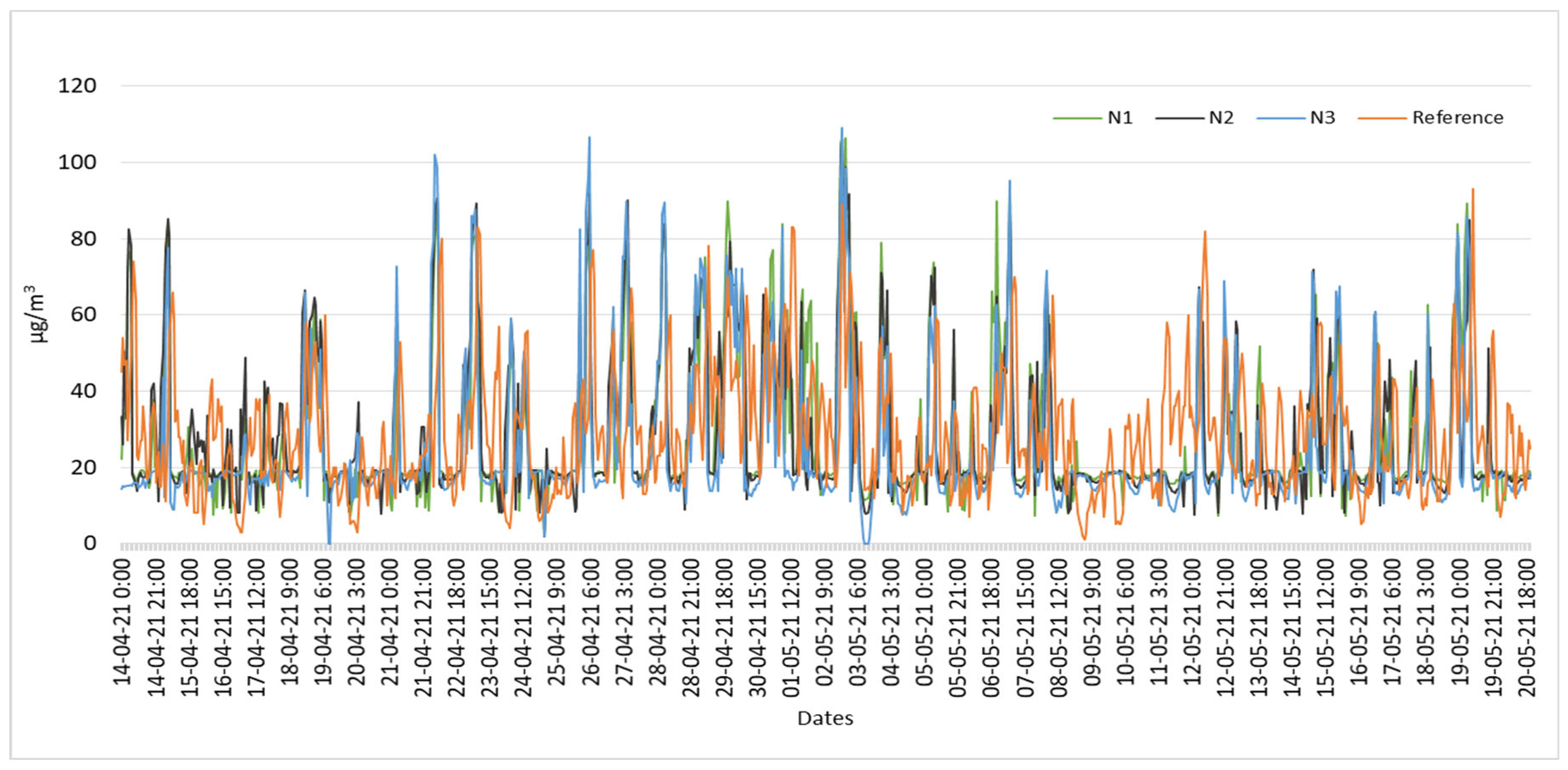
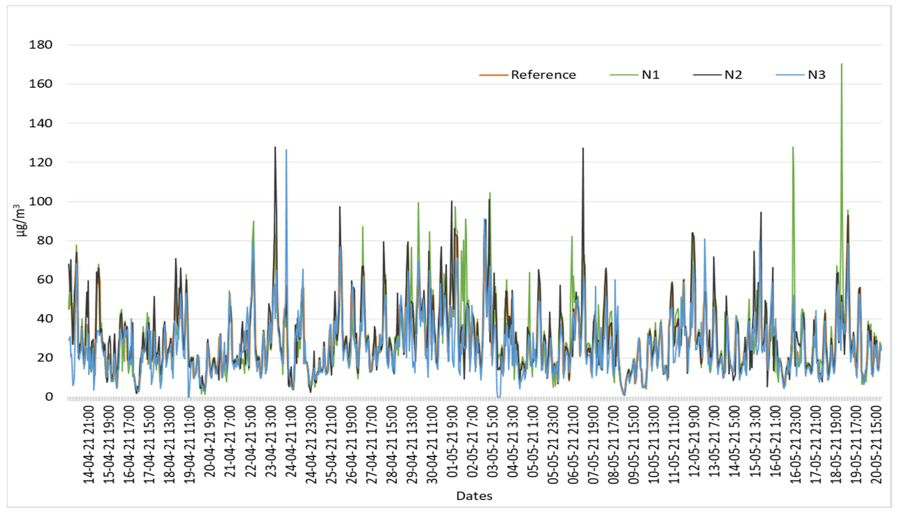
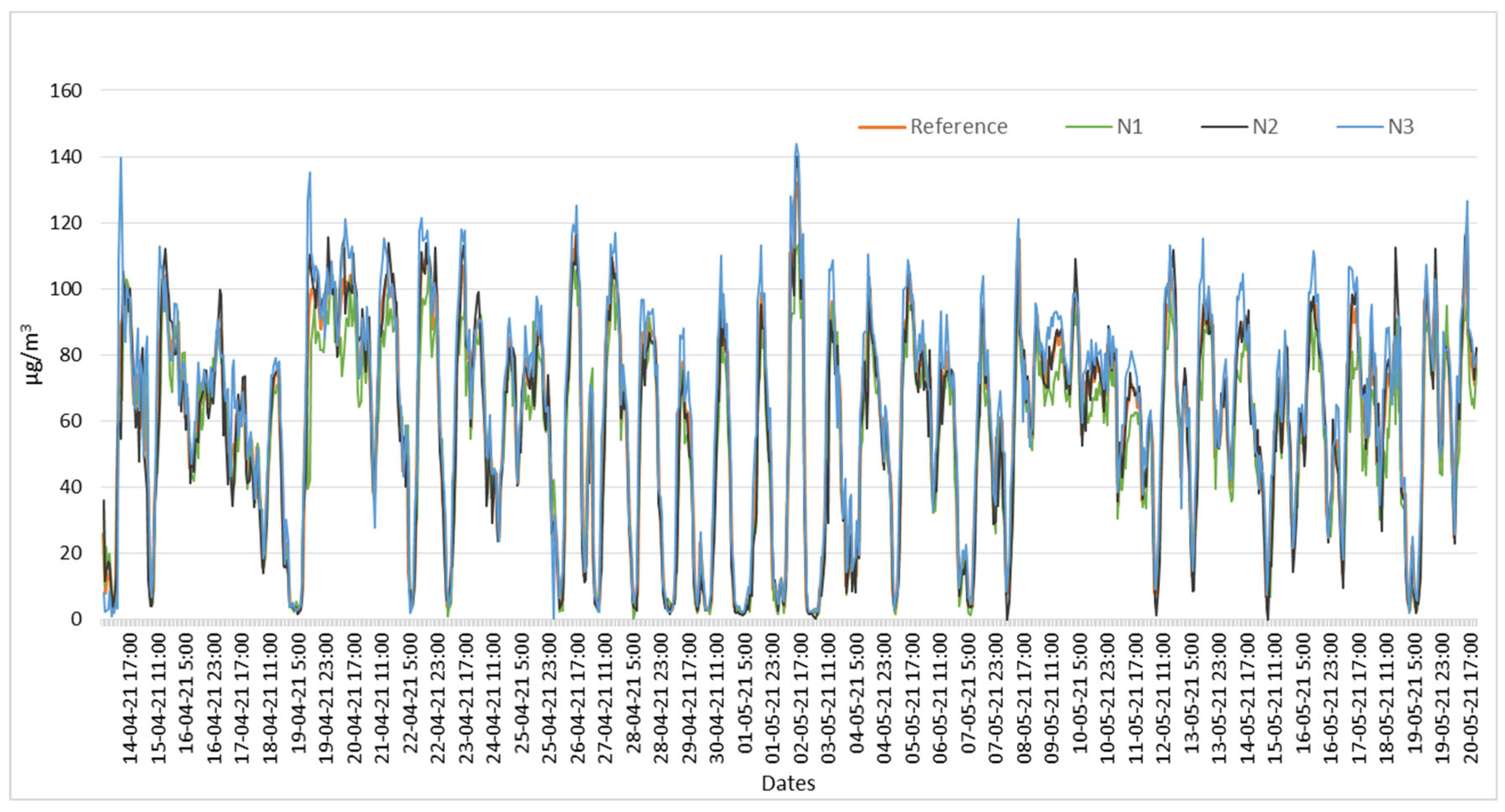
Figure 6.
NO2 time series of three LCS and reference.
Figure 6.
NO2 time series of three LCS and reference.
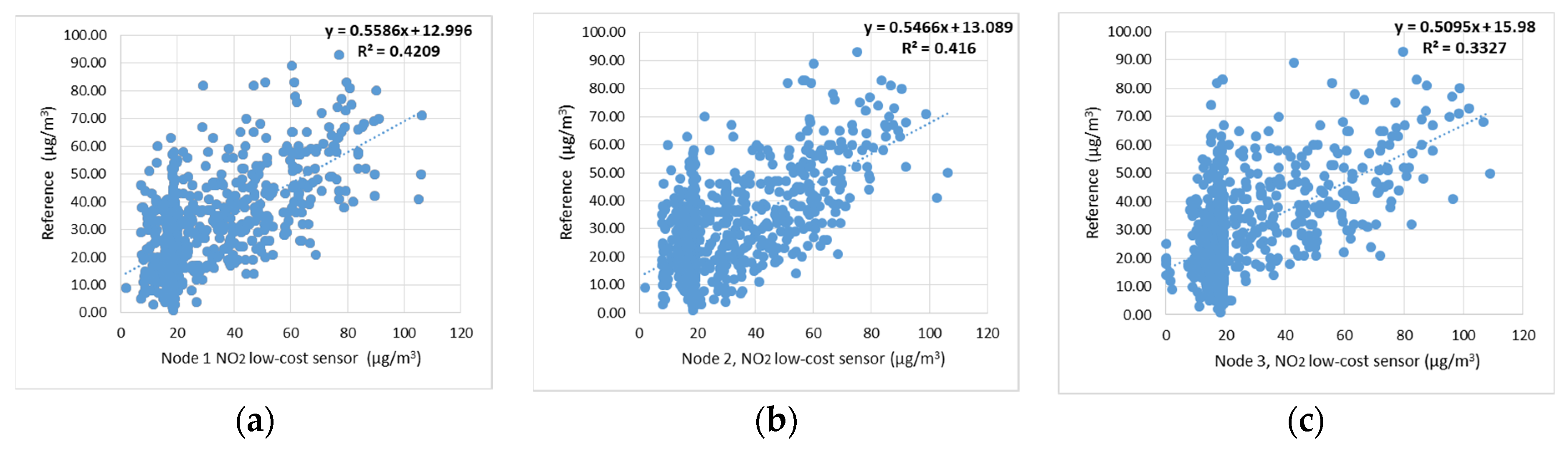
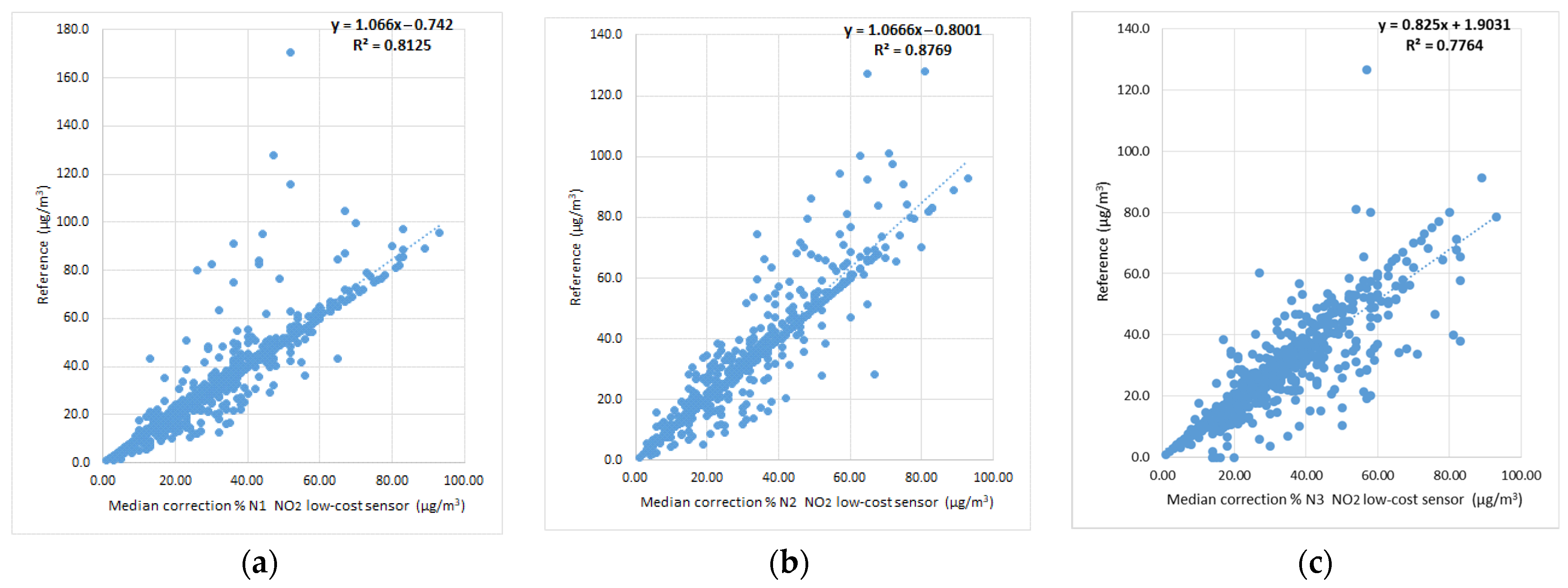
Figure 7.
Scatter plot of values of each LCS NO2 (N1, N2, N3) and reference. (a) Scatter plot of measurements of Node 1 NO2 LCS and reference, (b) Scatter plot of measurements of Node 2 NO2 LCS and reference, (c) Scatter plot of measurements of Node 3 NO2 LCS and reference.
Figure 7.
Scatter plot of values of each LCS NO2 (N1, N2, N3) and reference. (a) Scatter plot of measurements of Node 1 NO2 LCS and reference, (b) Scatter plot of measurements of Node 2 NO2 LCS and reference, (c) Scatter plot of measurements of Node 3 NO2 LCS and reference.
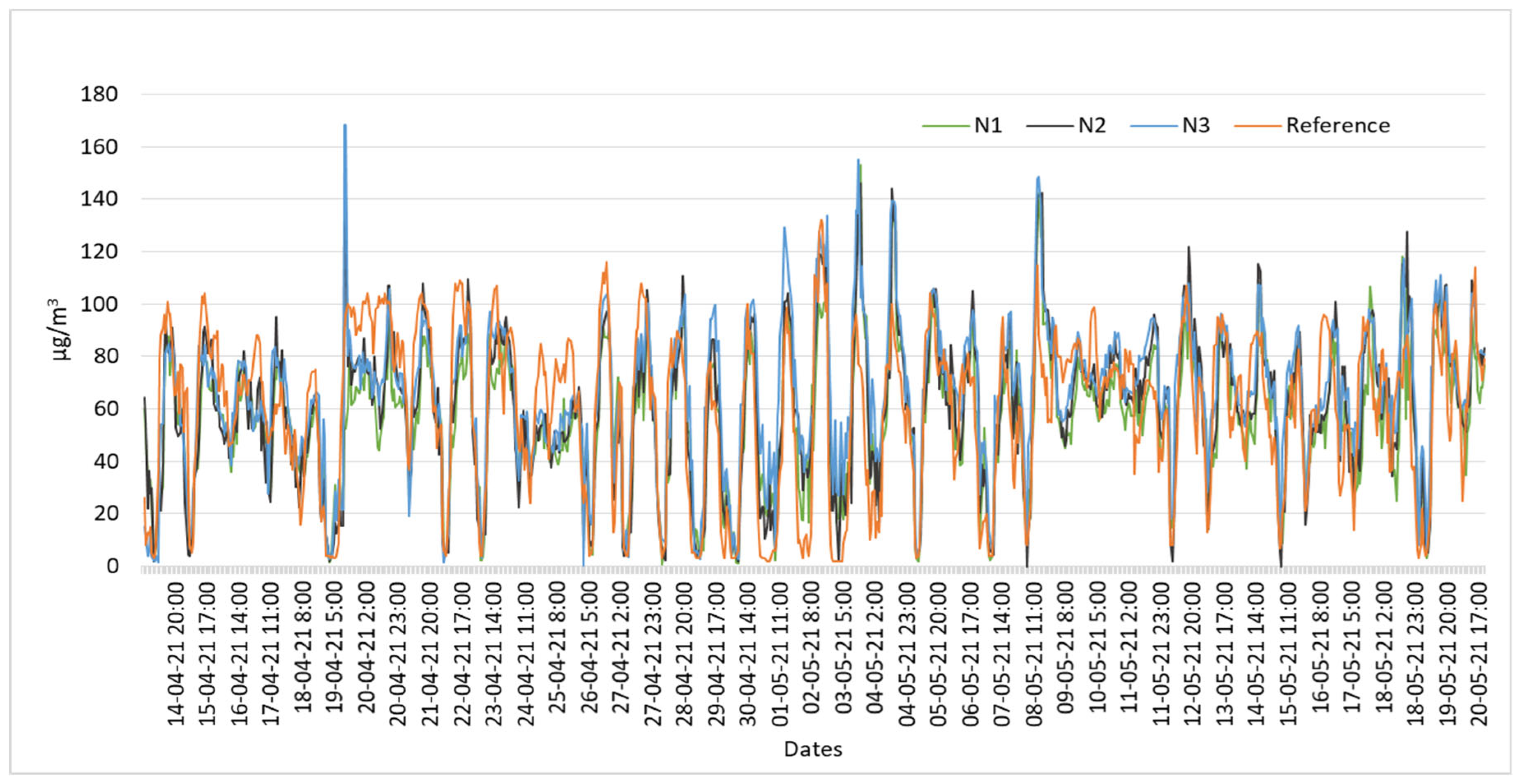
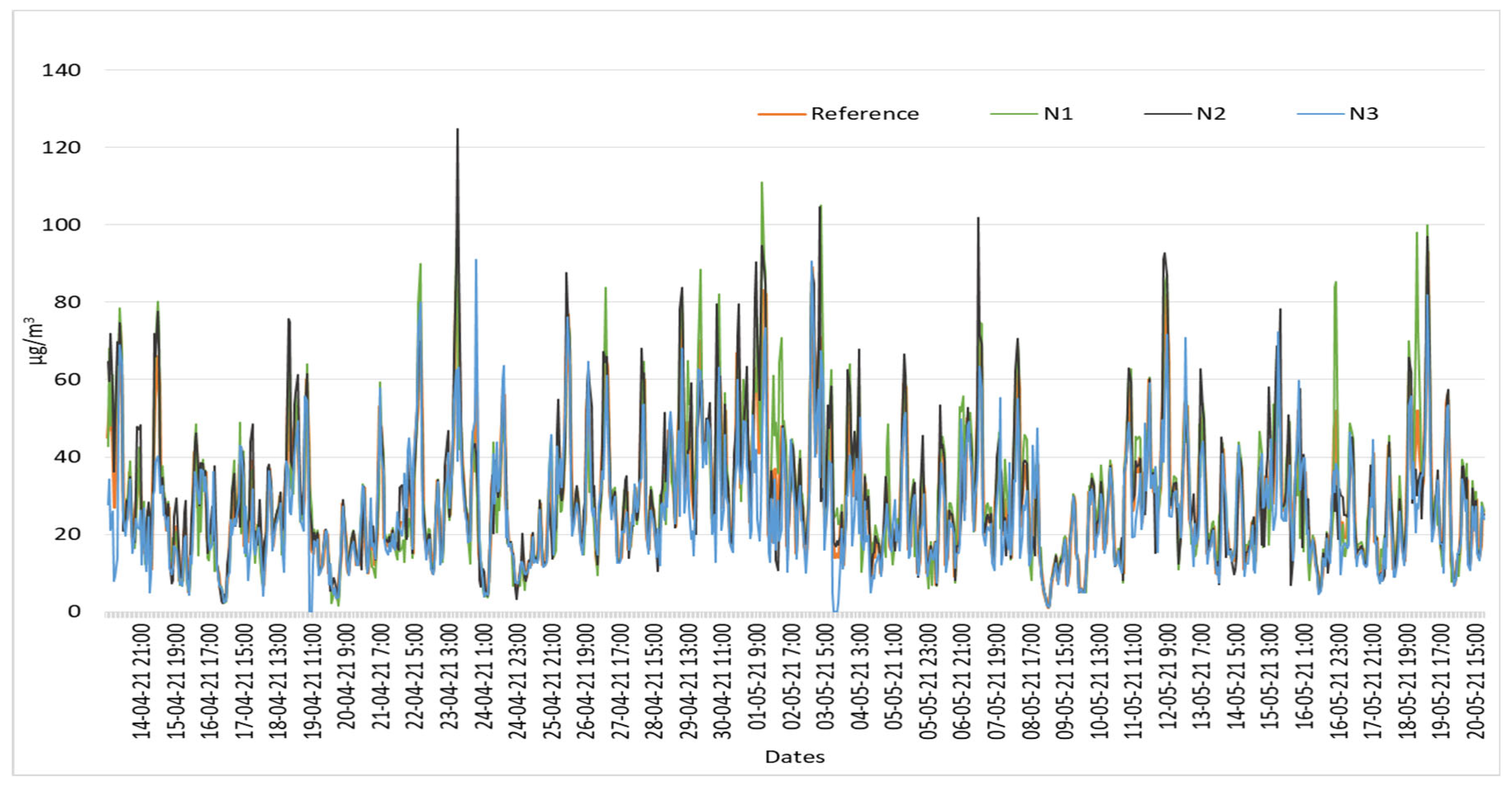
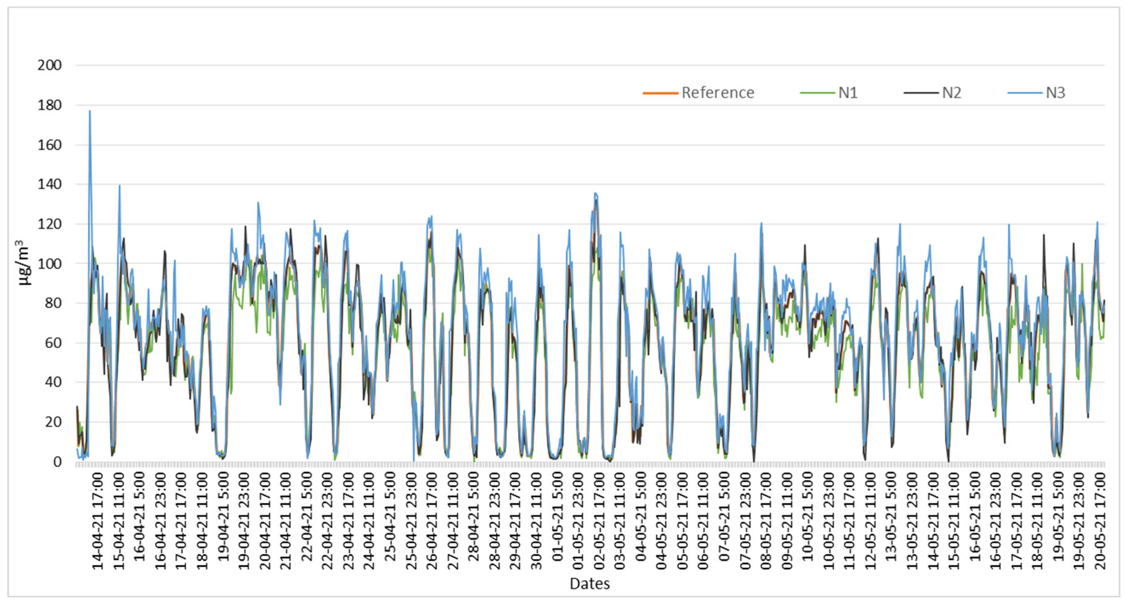
Figure 8.
O3 time series of three LCS and reference.
Figure 8.
O3 time series of three LCS and reference.
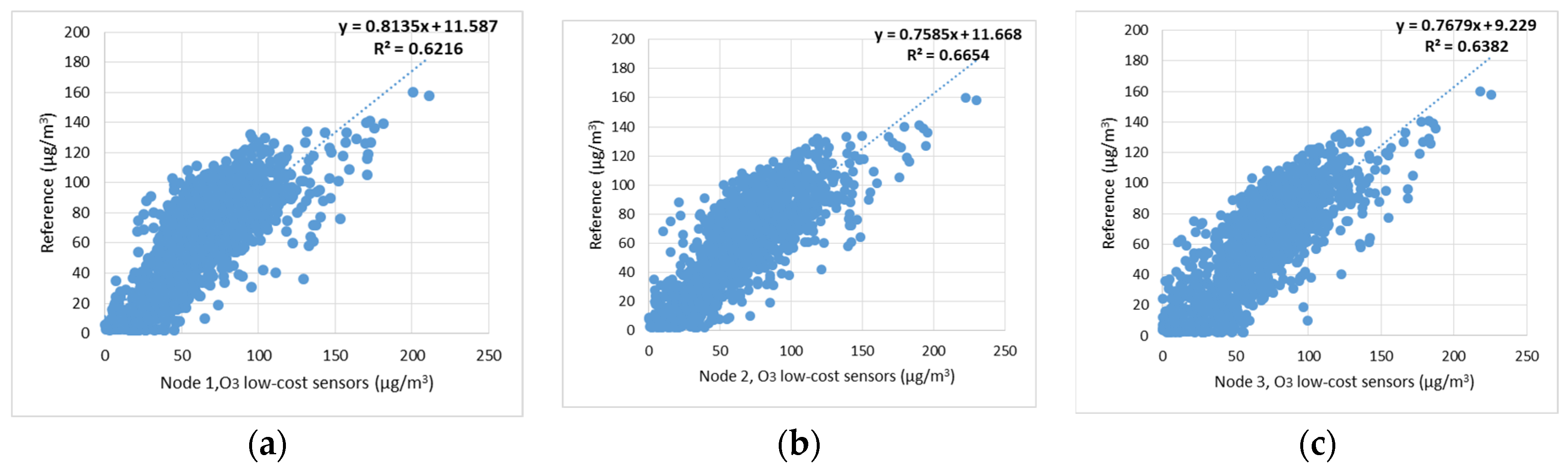
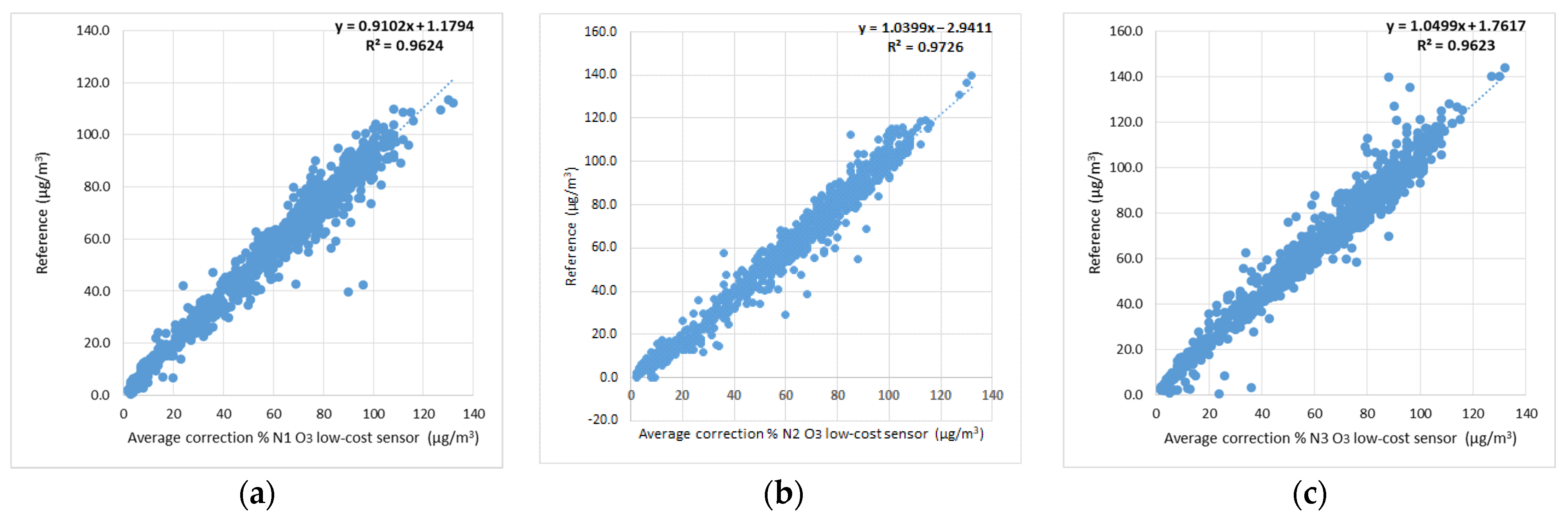
Figure 9.
Scatter plot of values of each LCS O3 (N1, N2, N3) and reference. (a) Scatter plot of measurements of Node 1 O3 LCS and reference, (b) Scatter plot of measurements of Node 2 O3 LCS and reference, (c) Scatter plot of measurements of Node 3 O3 LCS and reference.
Figure 9.
Scatter plot of values of each LCS O3 (N1, N2, N3) and reference. (a) Scatter plot of measurements of Node 1 O3 LCS and reference, (b) Scatter plot of measurements of Node 2 O3 LCS and reference, (c) Scatter plot of measurements of Node 3 O3 LCS and reference.
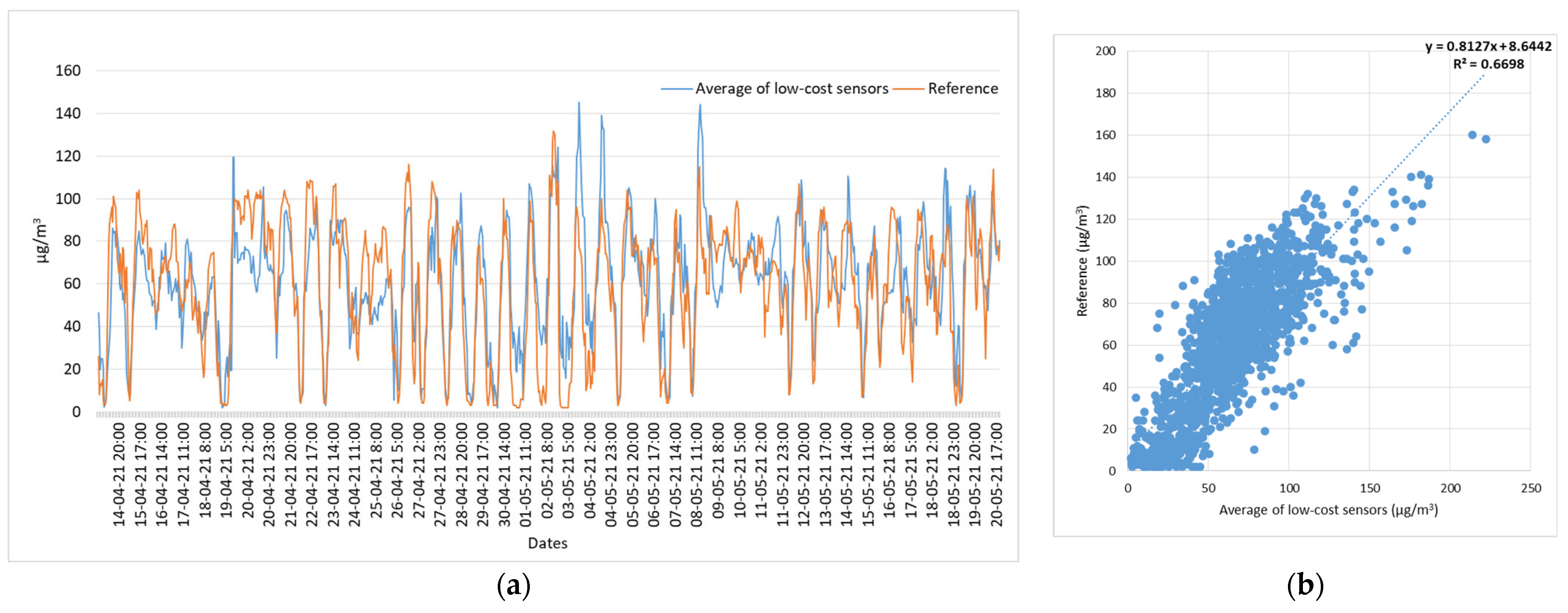
Figure 10.
Performance of average values of three low-cost nitrogen dioxide sensors and the reference values. (a) Time series of the average values and reference values of nitrogen dioxide concentration, (b) Scatter plot between the average and reference values of nitrogen dioxide concentration.
Figure 10.
Performance of average values of three low-cost nitrogen dioxide sensors and the reference values. (a) Time series of the average values and reference values of nitrogen dioxide concentration, (b) Scatter plot between the average and reference values of nitrogen dioxide concentration.
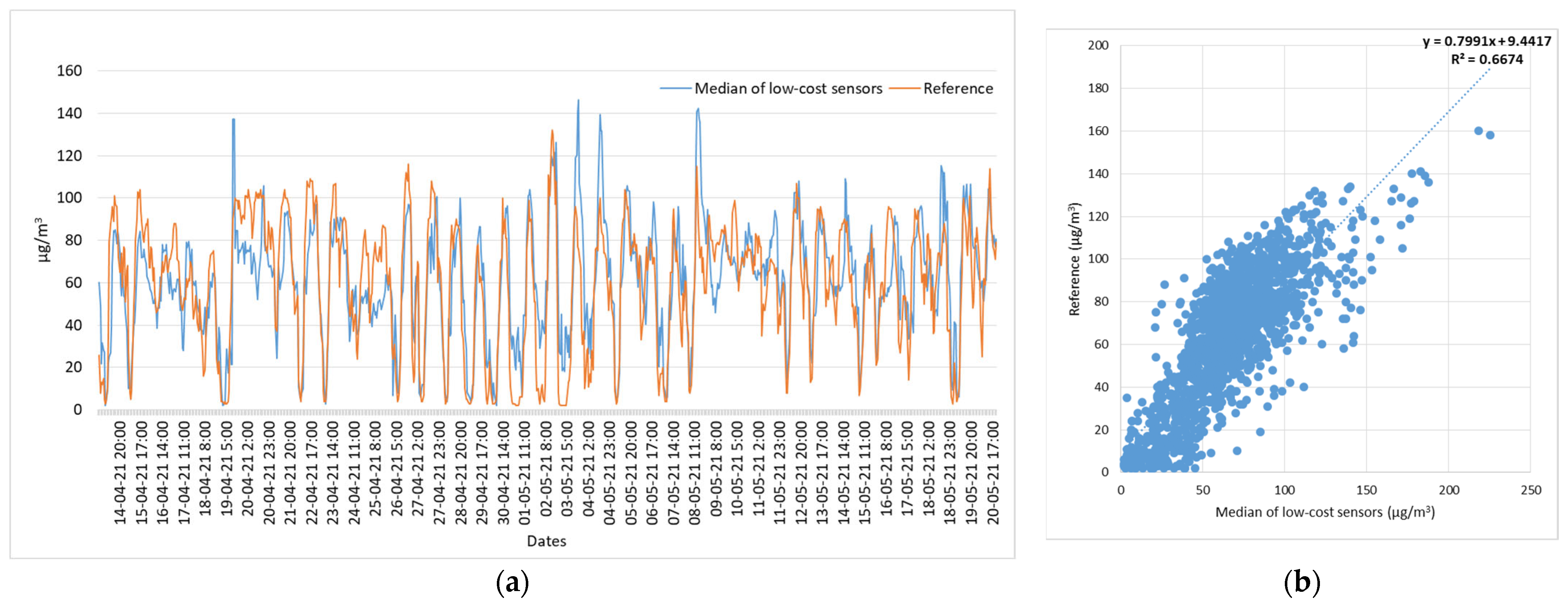
Figure 11.
Performance of median values of three low-cost nitrogen dioxide sensors and the reference values. (a) Time series of the median values and reference values of nitrogen dioxide concentration, (b) Scatter plot between the median and reference values of nitrogen dioxide concentration.
Figure 11.
Performance of median values of three low-cost nitrogen dioxide sensors and the reference values. (a) Time series of the median values and reference values of nitrogen dioxide concentration, (b) Scatter plot between the median and reference values of nitrogen dioxide concentration.
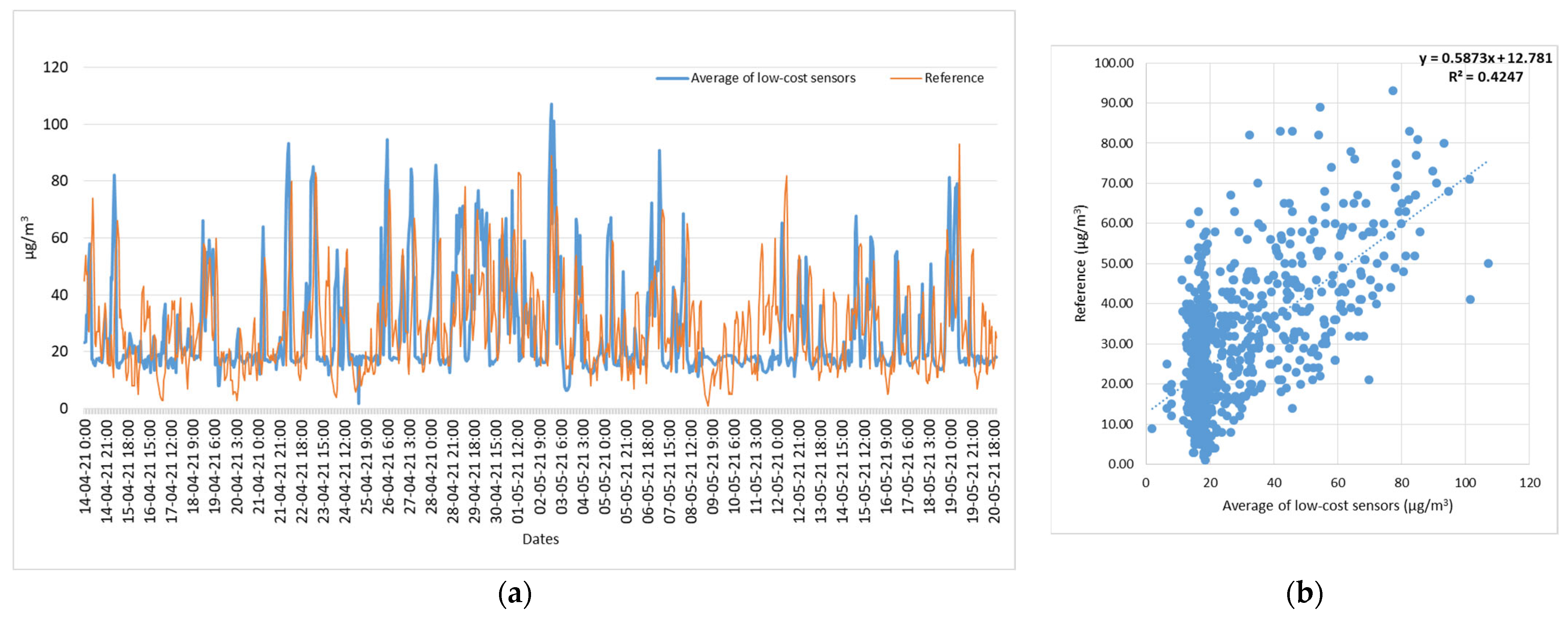
Figure 12.
Performance of average values of three low-cost ozone sensors and the reference values. (a) Time series of the average values and reference values of ozone concentration, (b) Correlation (R2) between the average and reference values of ozone concentration.
Figure 12.
Performance of average values of three low-cost ozone sensors and the reference values. (a) Time series of the average values and reference values of ozone concentration, (b) Correlation (R2) between the average and reference values of ozone concentration.
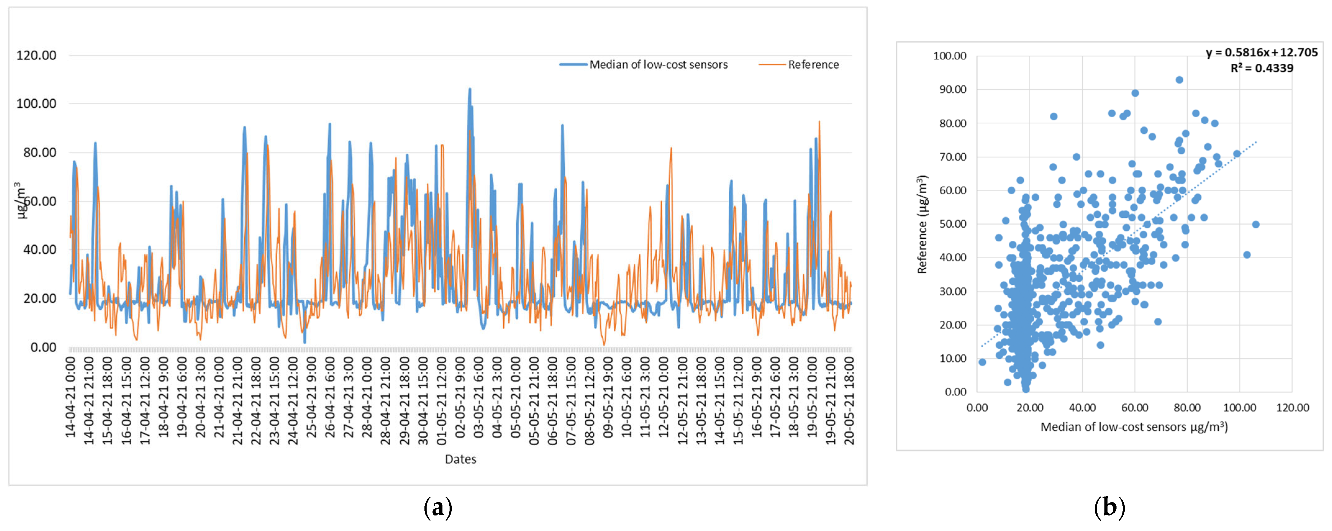
Figure 13.
Performance of median values of three low-cost ozone sensors and the reference values. (a) Time series of the median values and reference values of ozone concentration, (b) Correlation (R2) between the median and reference values of ozone concentration.
Figure 13.
Performance of median values of three low-cost ozone sensors and the reference values. (a) Time series of the median values and reference values of ozone concentration, (b) Correlation (R2) between the median and reference values of ozone concentration.
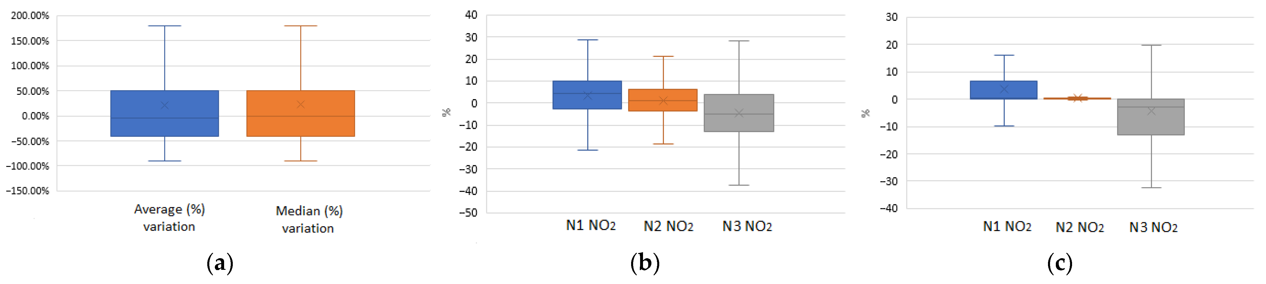
Figure 14.
Boxplots of NO2 LCS. (a) Total variation including the values of all three low-cost NO2 sensors, both the average and the median. (b) Variation of each low-cost NO2 sensor in relation to the percentage average values and reference values for each sensor. (c) Variation of each low-cost NO2 sensor in relation to the percentage median values and reference values for each sensor.
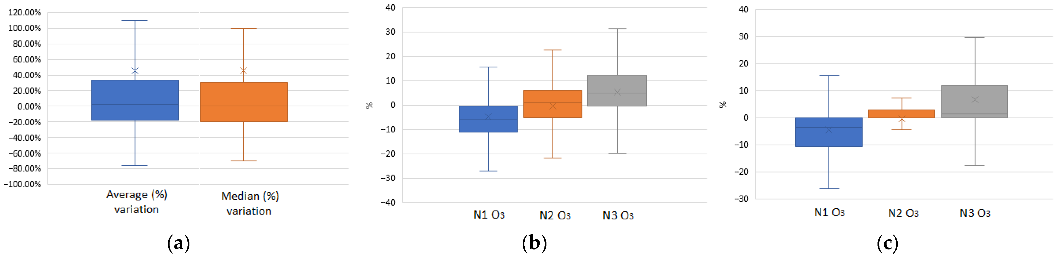
Figure 15.
Boxplots of O3 LCS. (a) Total variation including the values of all three low-cost O3 sensors, both the average and the median. (b) Variation of each low-cost O3 sensor in relation to the percentage average values and reference values for each sensor. (c) Variance of each low-cost O3 sensor in relation to the median average variance values versus the reference values for each sensor.
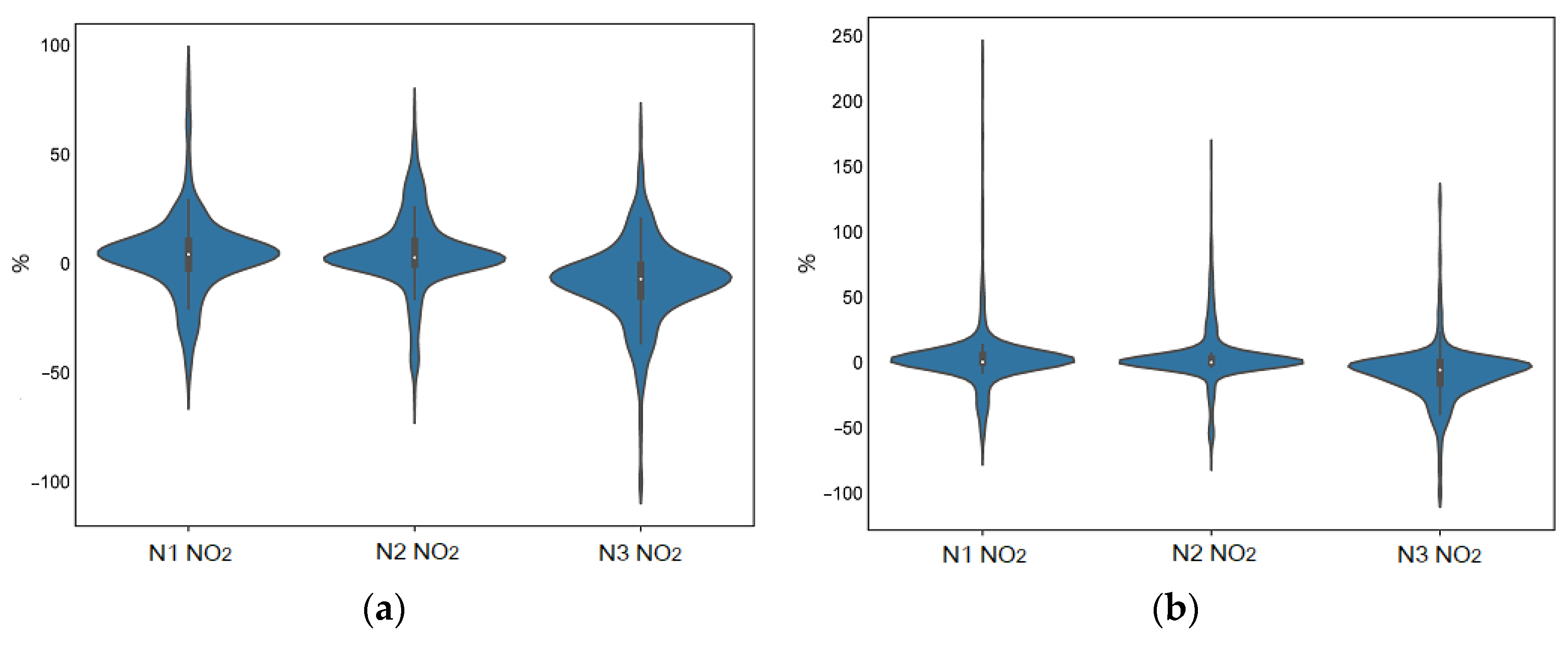
Figure 16.
Violin curves of NO2 LCS. (a) Percentage change distribution of average method of NO2 measurements. (b) Percentage change distribution of median method of NO2 measurements.
Figure 16.
Violin curves of NO2 LCS. (a) Percentage change distribution of average method of NO2 measurements. (b) Percentage change distribution of median method of NO2 measurements.
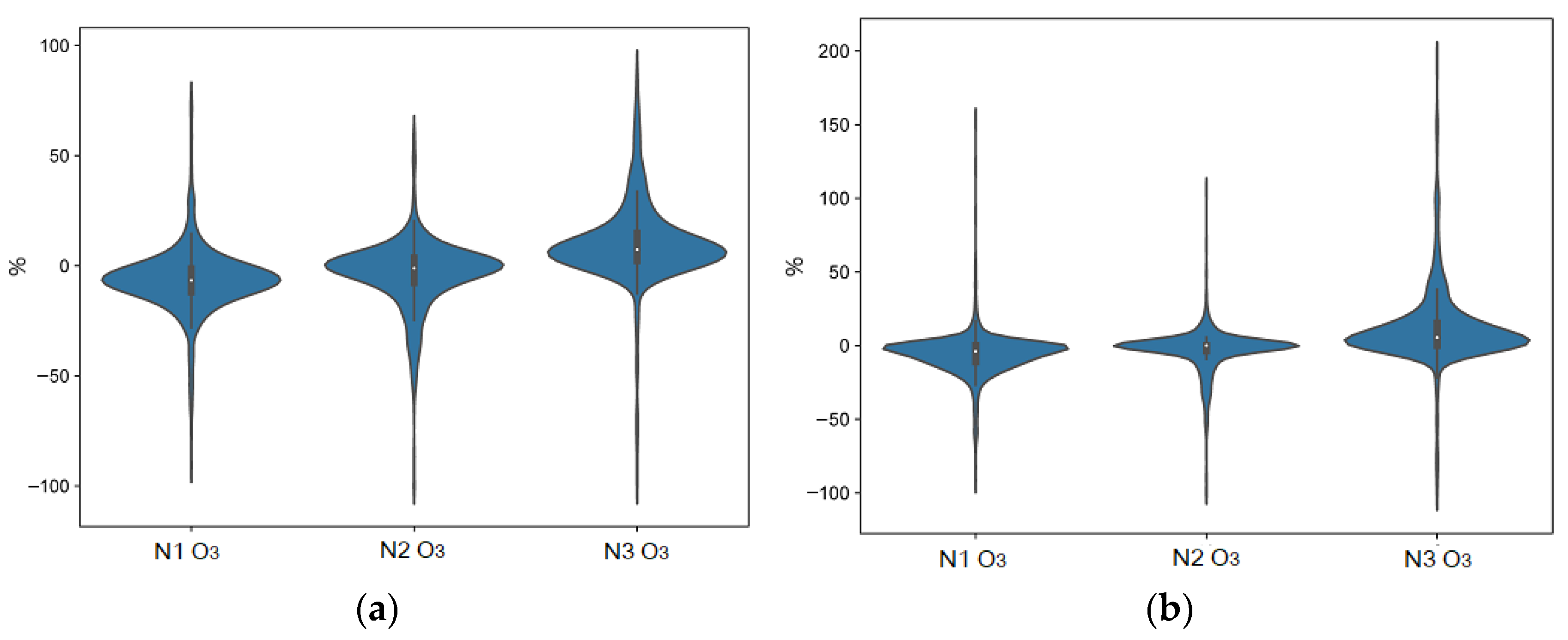
Figure 17.
Violin curves of O3 LCS. (a) Percentage change distribution of average method of O3 measurements. (b) Percentage change distribution of median method of O3 measurements.
Figure 17.
Violin curves of O3 LCS. (a) Percentage change distribution of average method of O3 measurements. (b) Percentage change distribution of median method of O3 measurements.
Figure 18.
Corrected values of each low-cost NO2 sensor using the average variation as correction factor in relation to the reference values.
Figure 18.
Corrected values of each low-cost NO2 sensor using the average variation as correction factor in relation to the reference values.
Figure 19.
Scatter plots of corrected values (average variation) in relation to the reference values of each NO2 sensor. (a) Scatter plot of corrected values in relation to the reference values of NO2 sensor of Node 1. (b) Scatter plot of corrected values in relation to the reference values of NO2 sensor of Node 2. (c) Scatter plot of corrected values in relation to the reference values of NO2 sensor of Node 3.
Figure 20.
Corrected values of each low-cost NO2 sensor using the median variation as correction factor in relation to the reference values.
Figure 20.
Corrected values of each low-cost NO2 sensor using the median variation as correction factor in relation to the reference values.
Figure 21.
Scatter plots of corrected values (median variation) in relation to the reference values of each NO2 sensor. (a) Scatter plot of median variation corrected values in relation to the reference values of NO2 sensor of Node 1. (b) Scatter plot of median variation corrected values in relation to the reference values of NO2 sensor of Node 2. (c) Scatter plot of median variation corrected values in relation to the reference values of NO2 sensor of Node 3.
Figure 22.
Corrected values of each low-cost O3 sensor using the average variation as correction factor in relation to the reference values.
Figure 22.
Corrected values of each low-cost O3 sensor using the average variation as correction factor in relation to the reference values.
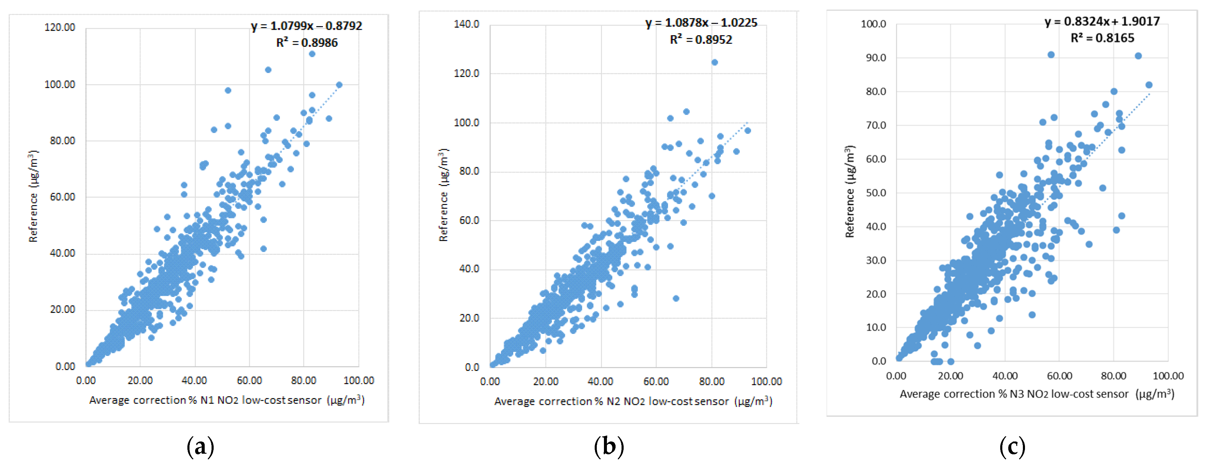
Figure 23.
Scatter plots of corrected values (average variation) in relation to the reference values of each O3 sensor. (a) Scatter plot of average variation corrected values in relation to the reference values of O3 sensor of Node 1. (b) Scatter plot of average variation corrected values in relation to the reference values of O3 sensor of Node 2. (c) Scatter plot of average variation corrected values in relation to the reference values of O3 sensor of Node 3.
Figure 24.
Corrected values of each low-cost O3 sensor using the median variation as correction factor in relation to the reference values.
Figure 24.
Corrected values of each low-cost O3 sensor using the median variation as correction factor in relation to the reference values.
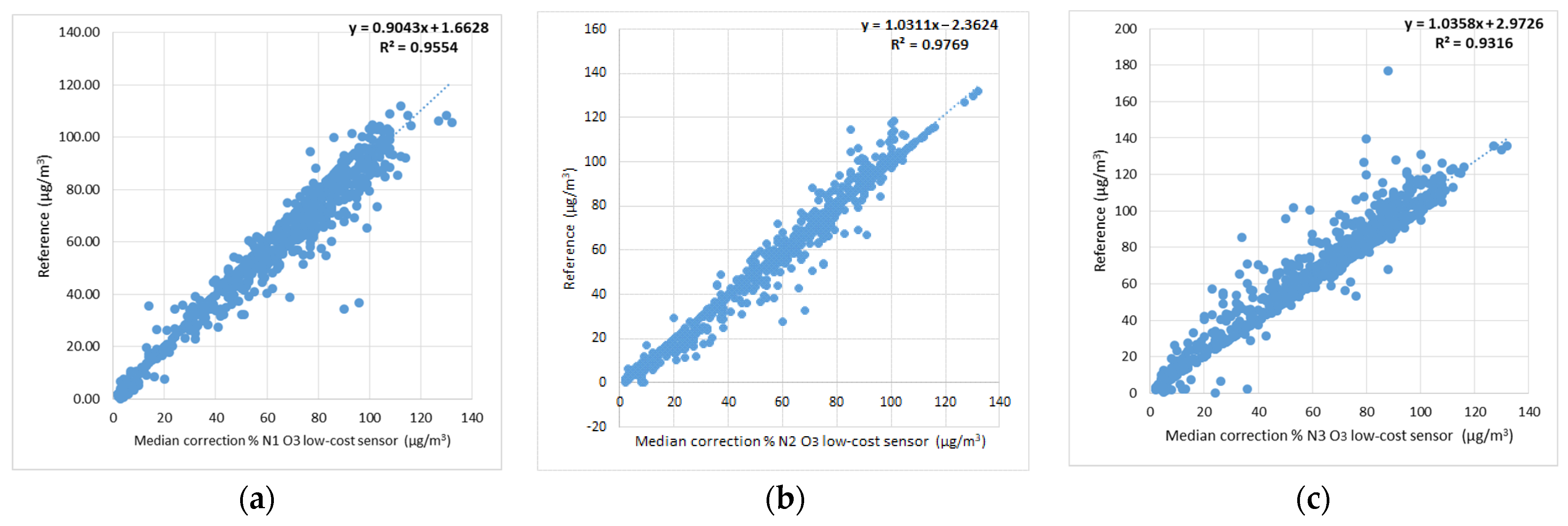
Figure 25.
Scatter plots, of corrected values (median variation) in relation to the reference values of each O3 sensor. (a) Scatter plot of median variation corrected values in relation to the reference values of O3 sensor of Node 1. (b) Scatter plot of median variation corrected values in relation to the reference values of O3 sensor of Node 2. (c) Scatter plot of median variation corrected values in relation to the reference values of O3 sensor of Node 3.
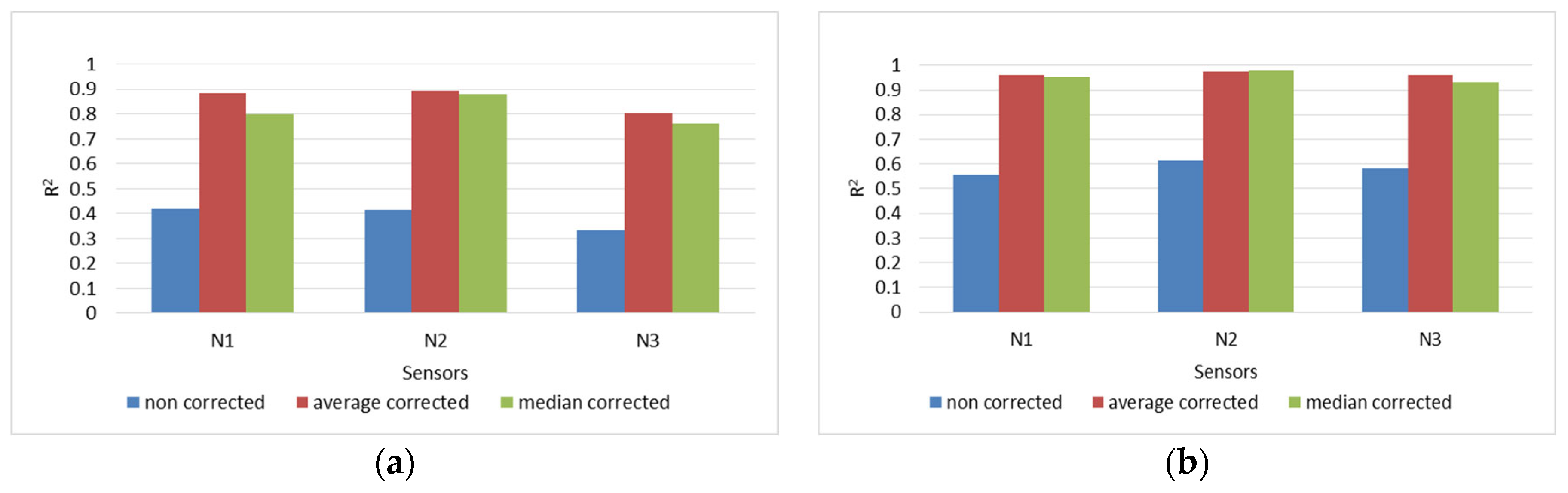
Figure 26.
LR correlations (R2) of non-corrected, corrected by average method, and corrected by median method, measurements in respect to the reference measurements. (a) LR correlations (R2) of NO2 gas concentrations, (b) LR correlations (R2) of O3 gas concentrations.
Figure 26.
LR correlations (R2) of non-corrected, corrected by average method, and corrected by median method, measurements in respect to the reference measurements. (a) LR correlations (R2) of NO2 gas concentrations, (b) LR correlations (R2) of O3 gas concentrations.
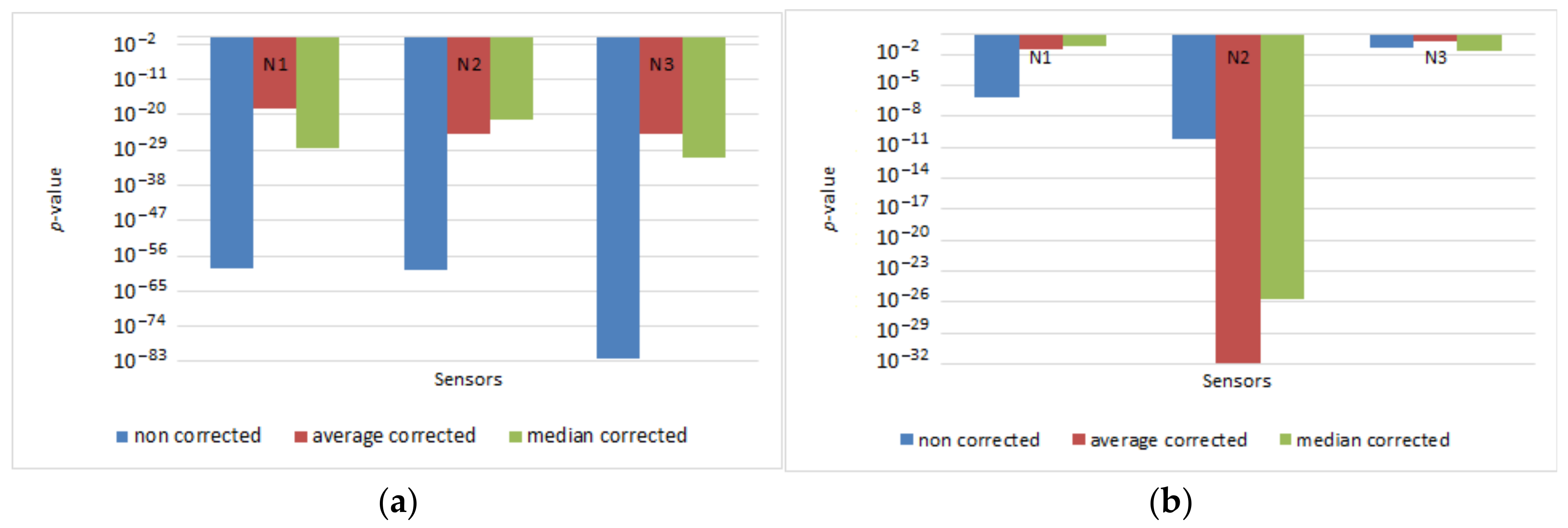
Figure 27.
Value of LR interception (p-value) of non-corrected, corrected by average method, and corrected by median method, measurements in respect to the reference measurements. (a) LR intercept (p-value) of NO2 gas concentrations, (b) LR interception (p-value) of O3 gas concentrations.
Figure 27.
Value of LR interception (p-value) of non-corrected, corrected by average method, and corrected by median method, measurements in respect to the reference measurements. (a) LR intercept (p-value) of NO2 gas concentrations, (b) LR interception (p-value) of O3 gas concentrations.
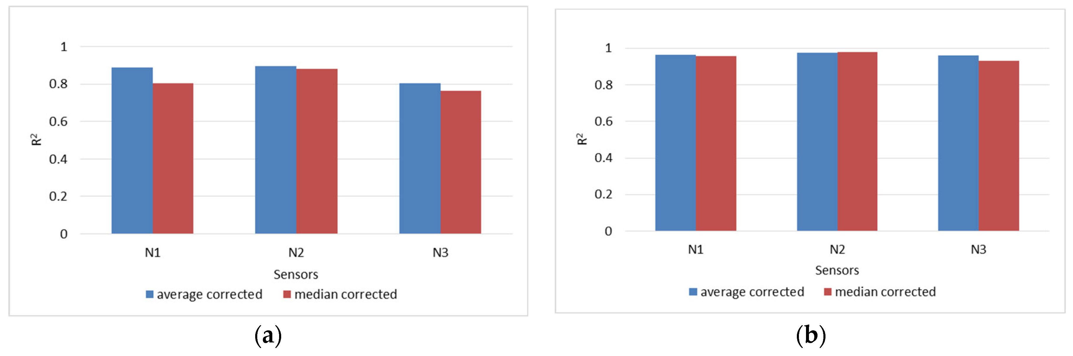
Figure 28.
MLR correlations (R2) of corrected by average method and corrected by median method, measurements in respect to the reference measurements. (a) MLR correlations (R2) of NO2 gas concentrations, (b) MLR correlations (R2) of O3 gas concentrations.
Figure 28.
MLR correlations (R2) of corrected by average method and corrected by median method, measurements in respect to the reference measurements. (a) MLR correlations (R2) of NO2 gas concentrations, (b) MLR correlations (R2) of O3 gas concentrations.
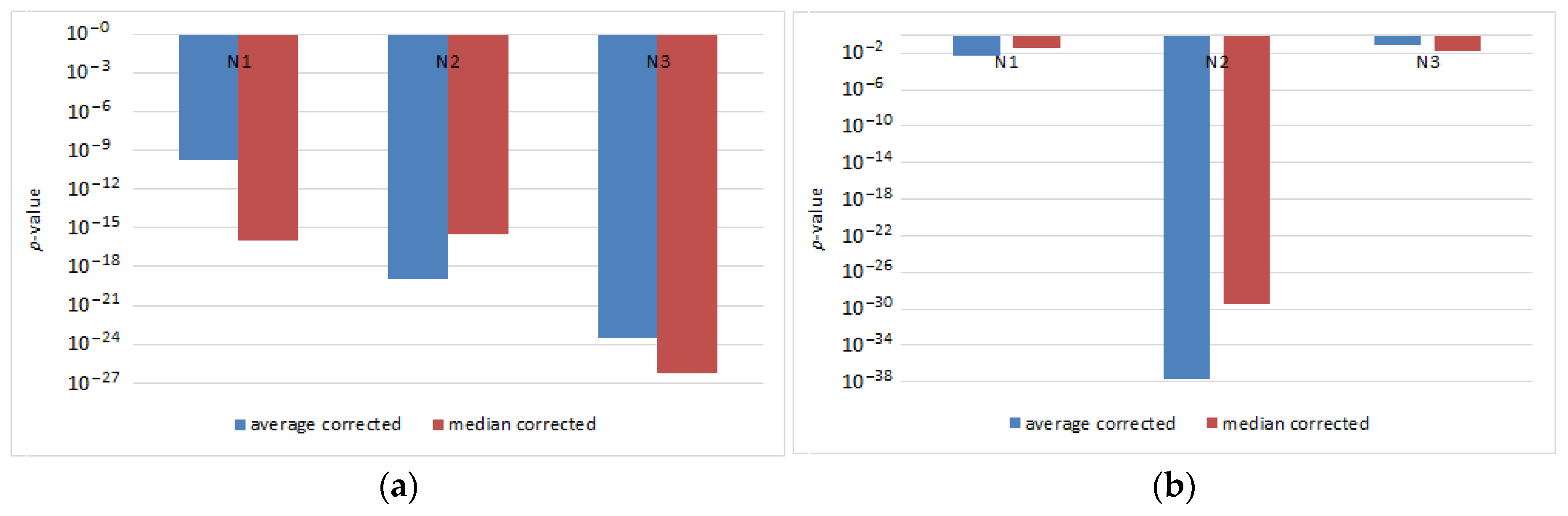
Figure 29.
Value of MLR interception (p-value) corrected by average method and corrected by median method, measurements in respect to the reference measurements. (a) MLR intercept (p-value) of NO2 gas concentrations, (b) MLR interception (p-value) of O3 gas concentrations.
Figure 29.
Value of MLR interception (p-value) corrected by average method and corrected by median method, measurements in respect to the reference measurements. (a) MLR intercept (p-value) of NO2 gas concentrations, (b) MLR interception (p-value) of O3 gas concentrations.
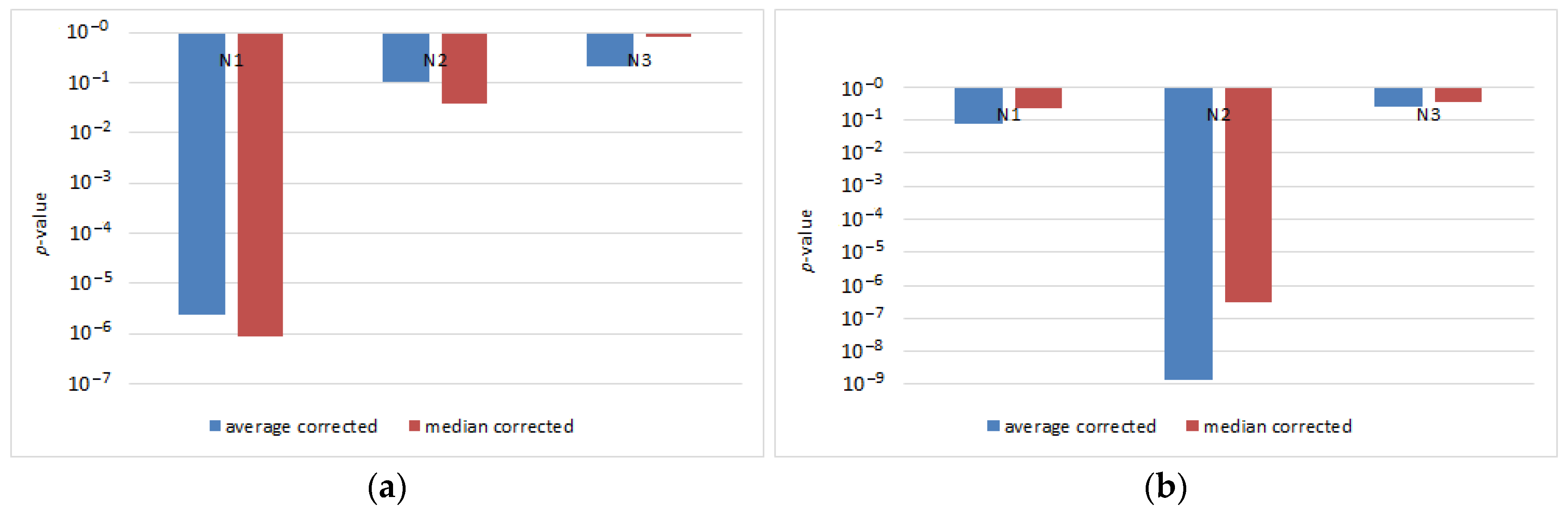
Figure 30.
Value of MLR percentage change (%) as a correction factor (p-value) of corrected by average method and corrected by median method, measurements in respect to the reference measurements. (a) MLR percentage change (%) as a correction factor (p-value) of NO2 gas concentrations, (b) MLR percentage change (%) as a correction factor (p-value) of O3 gas concentrations.
Table 1.
LR, reference values and N1, N2, N3 (non-corrected values) of NO2.
Table 1.
LR, reference values and N1, N2, N3 (non-corrected values) of NO2.
| Regression Statistics | N1 | N2 | N3 |
|---|
| Multiple R | 0.648 | 0.645 | 0.577 |
| R Square | 0.420 | 0.416 | 0.333 |
| Adjusted R Square | 0.420 | 0.415 | 0.332 |
| Standard Error | 12.192 | 12.241 | 13.082 |
| Observations | 886 | 886 | 886 |
| Significance F | 8.45 × 10−107 | 2.89 × 10−105 | 1.02 × 10−79 |
| Intercept (p-value) | 6.72 × 10−60 | 2.84 × 10−60 | 4.35 × 10−83 |
| NO2 Sensor (p-value) | 8.45 × 10−107 | 2.89× 10−105 | 1.02 × 10−79 |
Table 2.
LR, reference values and the average, and median values of non-corrected values (average or median variation) of NO2 (N1, N2, N3).
Table 2.
LR, reference values and the average, and median values of non-corrected values (average or median variation) of NO2 (N1, N2, N3).
| Regression Statistics | Average N1, N2, N3 | Median N1, N2, N3 |
|---|
| Multiple R | 0.652 | 0.659 |
| R Square | 0.425 | 0.434 |
| Adjusted R Square | 0.424 | 0.434 |
| Standard Error | 12.142 | 12.045 |
| Observations | 886 | 886 |
| Significance F | 2.19 × 10−108 | 1.723 × 10−111 |
| Intercept (p-value) | 4.98 × 10−57 | 1.23 × 10−57 |
| Aver. N1, N2, N3 (p-value) | 2.19 × 10−108 | |
| Med. N1, N2, N3 (p-value) | | 1.72 × 10−111 |
Table 3.
LR, reference values and average variation corrected values of NO2 (N1, N2, N3).
Table 3.
LR, reference values and average variation corrected values of NO2 (N1, N2, N3).
| Regression Statistics | N1 | N2 | N3 |
|---|
| Multiple R | 0.941 | 0.946 | 0.896 |
| R Square | 0.886 | 0.895 | 0.802 |
| Adjusted R Square | 0.886 | 0.894 | 0.802 |
| Standard Error | 5.412 | 5.199 | 7.117 |
| Observations | 886 | 886 | 886 |
| Significance F | 0 | 0 | 0 |
| Intercept (p-value) | 3.66× 10⁻¹⁹ | 9.35× 10⁻²⁶ | 1.86 × 10⁻²⁵ |
| Aver. Corr. (p-value) | 0 | 0 | 0 |
Table 4.
LR, reference values and median variation corrected values of NO2 (N1, N2, N3).
Table 4.
LR, reference values and median variation corrected values of NO2 (N1, N2, N3).
| Regression Statistics | N1 | N2 | N3 |
|---|
| Multiple R | 0.894 | 0.939 | 0.874 |
| R Square | 0.799 | 0.882 | 0.763 |
| Adjusted R Square | 0.799 | 0.882 | 0.763 |
| Standard Error | 7.172 | 5.496 | 7.790 |
| Observations | 886 | 886 | 886 |
| Significance F | 0 | 0 | 6.17 × 10−279 |
| Intercept (p-value) | 4.07 × 10⁻²⁹ | 3.89 × 10⁻²² | 1.61 × 10⁻³¹ |
| Med. Corr. (p-value) | 0 | 0 | 6.17 × 10−279 |
Table 5.
LR, reference values and N1, N2, N3 (non-corrected values) of O3.
Table 5.
LR, reference values and N1, N2, N3 (non-corrected values) of O3.
| | Regression Statistics | N2 | N3 |
|---|
| Multiple R | 0.748 | 0.785 | 0.764 |
| R Square | 0.559 | 0.617 | 0.584 |
| Adjusted R Square | 0.559 | 0.617 | 0.584 |
| Standard Error | 20.146 | 18.776 | 19.569 |
| Observations | 886 | 886 | 886 |
| Significance F | 1.95 × 10−159 | 1.68 × 10−186 | 1.32 × 10−170 |
| Intercept (p-value) | 7.40 × 10⁻⁷ | 6.87 × 10⁻¹¹ | 0.0438 |
| O3 Sensor (p-value) | 1.95 × 10−159 | 1.68 × 10−186 | 1.32 × 10−170 |
Table 6.
LR, reference values and the average, and median values of non-corrected values (average or median variation) of O3 (N1, N2, N3).
Table 6.
LR, reference values and the average, and median values of non-corrected values (average or median variation) of O3 (N1, N2, N3).
| Regression Statistics | Average N1, N2, N3 | Median N1, N2, N3 |
|---|
| Multiple R | 0.786 | 0.782 |
| R Square | 0.618 | 0.612 |
| Adjusted R Square | 0.618 | 0.611 |
| Standard Error | 18.748 | 18.900 |
| Observations | 887 | 887 |
| Significance F | 3.68 × 10−187 | 4.67 × 10−184 |
| Intercept (p-value) | 0.005 | 0.0002 |
| Aver. N1, N2, N3 (p-value) | 3.68 × 10−187 | |
| Med. N1, N2, N3 (p-value) | | 4.67 × 10−184 |
Table 7.
LR, reference values and average variation corrected values of O3 (N1, N2, N3).
Table 7.
LR, reference values and average variation corrected values of O3 (N1, N2, N3).
| Regression Statistics | N1 | N2 | N3 |
|---|
| Multiple R | 0.981 | 0.986 | 0.981 |
| R Square | 0.963 | 0.973 | 0.962 |
| Adjusted R Square | 0.963 | 0.973 | 0.962 |
| Standard Error | 5.863 | 4.989 | 5.883 |
| Observations | 886 | 886 | 886 |
| Significance F | 0 | 0 | 0 |
| Intercept (p-value) | 0.03 | 1.34 × 10⁻³² | 0.15 |
| Aver. Corr. (p-value) | 0 | 0 | 0 |
Table 8.
LR, reference values and median variation corrected values of O3 (N1, N2, N3).
Table 8.
LR, reference values and median variation corrected values of O3 (N1, N2, N3).
| Regression Statistics | N1 | N2 | N3 |
|---|
| Multiple R | 0.978 | 0.988 | 0.965 |
| R Square | 0.956 | 0.977 | 0.932 |
| Adjusted R Square | 0.956 | 0.977 | 0.932 |
| Standard Error | 6.378 | 4.591 | 7.930 |
| Observations | 886 | 886 | 886 |
| Significance F | 0 | 0 | 0 |
| Intercept (p-value) | 0.069 | 1.85 × 10⁻²⁶ | 0.018 |
| Med. Corr. (p-value) | 0 | 0 | 0 |
Table 9.
MLR, reference values, and the affection of average and median percentage changes in non-corrected values (average or median variation) of NO2 (N1, N2, N3).
Table 9.
MLR, reference values, and the affection of average and median percentage changes in non-corrected values (average or median variation) of NO2 (N1, N2, N3).
| Regression Statistics | Average N1, N2, N3 | Median N1, N2, N3 |
|---|
| Multiple R | 0.789 | 0.795 |
| R Square | 0.622 | 0.632 |
| Adjusted R Square | 0.622 | 0.631 |
| Standard Error | 9.847 | 9.724 |
| Observations | 886 | 886 |
| Significance F | 1.90 × 10−187 | 2.84 × 10−192 |
| Intercept (p-value) | 4.57 × 10−129 | 1.20 × 10−131 |
| Aver. N1, N2, N3 (p-value) | 3.73 × 10−164 | |
| % Average—Ref (p-value) | 1.24 × 10−82 | |
| Med. N1, N2, N3 (p-value) | | 3.91 × 10−169 |
| % Median—Ref (p-value) | | 2.29 × 10−84 |
Table 10.
MLR, reference values, and average variation corrected values of NO2 (N1, N2, N3).
Table 10.
MLR, reference values, and average variation corrected values of NO2 (N1, N2, N3).
| Regression Statistics | N1 | N2 | N3 |
|---|
| Multiple R | 0.943 | 0.946 | 0.896 |
| R Square | 0.889 | 0.895 | 0.803 |
| Adjusted R Square | 0.8885.348 | 0.895 | 0.802 |
| Standard Error | 886 | 5.194 | 7.114 |
| Observations | | 886 | 886 |
| Significance F | 0 | 0 | 0 |
| Intercept (p-value) | 1.67 × 10⁻¹⁰ | 1.16 × 10⁻¹⁹ | 2.87 × 10⁻²⁴ |
| Aver. Corr. (p-value) | 0 | 0 | 0 |
| % Average—Ref (p-value) | 2.45 × 10⁻⁶ | 0.10 | 0.21 |
Table 11.
MLR, reference values, and median variation corrected values of NO2 (N1, N2, N3).
Table 11.
MLR, reference values, and median variation corrected values of NO2 (N1, N2, N3).
| Regression Statistics | N1 | N2 | N3 |
|---|
| Multiple R | 0.897 | 0.940 | 0.874 |
| R Square | 0.805 | 0.882 | 0.763 |
| Adjusted R Square | 0.804 | 0.883 | 0.763 |
| Standard Error | 7.078 | 5.486 | 7.794 |
| Observations | 886 | 886 | 886 |
| Significance F | 0 | 0 | 4.00 × 10−277 |
| Intercept (p-value) | 9.38 × 10⁻¹⁷ | 3.01 × 10⁻¹⁶ | 5.98 × 10⁻²⁷ |
| Median Corr. (p-value) | 0 | 0 | 7.94 × 10−275 |
| % Median—Ref (p-value) | 8.86 × 10⁻⁷ | 0.037 | 0.80 |
Table 12.
MLR, reference values, and the affection of average and median percentage change in non-corrected values (average or median variation) of O3 (N1, N2, N3).
Table 12.
MLR, reference values, and the affection of average and median percentage change in non-corrected values (average or median variation) of O3 (N1, N2, N3).
| Regression Statistics | Average N1, N2, N3 | Median N1, N2, N3 |
|---|
| Multiple R | 0.839 | 0.837 |
| R Square | 0.704 | 0.701 |
| Adjusted R Square | 0.703 | 0.701 |
| Standard Error | 16.514 | 16.589 |
| Observations | 887 | 887 |
| Significance F | 2.03 × 10−234 | 1.10 × 10−232 |
| Intercept (p-value) | 1.10 × 10⁻²³ | 2.92 × 10⁻²⁷ |
| Aver. N1, N2, N3 (p-value) | 7.60 × 10−190 | |
| % Average—Ref (p-value) | 6.55 × 10−51 | |
| Med. N1, N2, N3 (p-value) | | 1.03 × 10−189 |
| % Median—Ref (p-value) | | 2.80 × 10−52 |
Table 13.
MLR, reference values, and average variation corrected values of O3 (N1, N2, N3).
Table 13.
MLR, reference values, and average variation corrected values of O3 (N1, N2, N3).
| Regression Statistics | N1 | N2 | N3 |
|---|
| Multiple R | 0.981 | 0.987 | 0.981 |
| R Square | 0.963 | 0.974 | 0.962 |
| Adjusted R Square | 0.963 | 0.974 | 0.962 |
| Standard Error | 5.856 | 4.889 | 5.882 |
| Observations | 886 | 886 | 886 |
| Significance F | 0 | 0 | 0 |
| Intercept (p-value) | 0.005 | 1.97 × 10−38 | 0.067 |
| Aver. Corr. (p-value) | 0 | 0 | 0 |
| % Average—Ref (p-value) | 0.08 | 1.35 × 10⁻⁹ | 0.257 |
Table 14.
MLR, reference values, and median variation corrected values of O3 (N1, N2, N3).
Table 14.
MLR, reference values, and median variation corrected values of O3 (N1, N2, N3).
| Regression Statistics | N1 | N2 | N3 |
|---|
| Multiple R | 0.978 | 0.989 | 0.965 |
| R Square | 0.956 | 0.977 | 0.932 |
| Adjusted R Square | 0.956 | 0.977 | 0.932 |
| Standard Error | 6.377 | 4.525 | 7.931 |
| Observations | 886 | 886 | 886 |
| Significance F | 0 | 0 | 0 |
| Intercept (p-value) | 0.031 | 2.70 × 10⁻³⁰ | 0.018 |
| Median Corr. (p-value) | 0 | 0 | 0 |
| % Median—Ref (p-value) | 0.236 | 3.00 × 10⁻⁷ | 0.369 |
Table 15.
Comparison of correlation degree of our work and published works.
Table 15.
Comparison of correlation degree of our work and published works.
| Gas Pollutant | Calibration Method | References | R2 |
|---|
| NO2 | ANN | Spinelle et al. [1], Wastine et al. [34] | 0.94 |
| LINEAR | Wastine et al. [34], Castell et al. [35],
Cross et al. [29] | 0.17 |
| MLR | Spinelle et al. [1], Karagulian et al. [36], Wei et al. [37] | 0.81 |
| Average/Median | Our work | 0.78–0.87 |
| O3 | ANN | Spinelle et al. [1], Wastine et al. [34] | 0.89 |
| LINEAR | Wastine et al. [34], Castell et al. [35],
Cross et al. [29] | 0.53 |
| MLR | Spinelle et al. [1], Karagulian et al. [36], Wei et al. [37] | 0.91 |
| Average/Median | Our work | 0.93–0.96 |
Table 16.
MAD of non-corrected, average variation corrected, and median variation corrected values of each LCS.
Table 16.
MAD of non-corrected, average variation corrected, and median variation corrected values of each LCS.
| MAD | N1 NO2 | N2 NO2 | N3 NO2 | N1 O3 | N2 O3 | N3 O3 |
|---|
| Non-corrected | 2.1 | 3.2 | 2.6 | 15.3 | 18.6 | 17.1 |
| Average corrected | 9.8 | 10.3 | 8.9 | 19.5 | 21.8 | 21.1 |
| Median corrected | 9.7 | 10.2 | 9.0 | 18.6 | 21.8 | 21.4 |
Table 17.
MSE of non-corrected, average variation corrected, and median variation corrected values of each LCS.
Table 17.
MSE of non-corrected, average variation corrected, and median variation corrected values of each LCS.
| MSE | N1 NO2 | N2 NO2 | N3 NO2 | N1 O3 | N2 O3 | N3 O3 |
|---|
| Non-corrected | 216.4 | 223.2 | 265.0 | 418.8 | 375.3 | 438.3 |
| Average corrected | 37.8 | 38.7 | 59.6 | 54.2 | 29.3 | 64.8 |
| Median corrected | 67.2 | 39.0 | 72.6 | 59.3 | 24.0 | 100.3 |
Table 18.
MAPE of non-corrected, average variation corrected, and median variation corrected values of each LCS.
Table 18.
MAPE of non-corrected, average variation corrected, and median variation corrected values of each LCS.
| MAPE | N1 NO2 | N2 NO2 | N3 NO2 | N1 O3 | N2 O3 | N3 O3 |
|---|
| Non-corrected | 49.0 | 52.7 | 50.8 | 62.5 | 56.2 | 81.1 |
| Average corrected | 12.9 | 11.7 | 14.8 | 11.2 | 9.9 | 13.9 |
| Median corrected | 10.5 | 9.1 | 13.81 | 9.1 | 7.0 | 14.8 |
Table 19.
RMSE of non-corrected, average variation corrected, and median variation corrected values of each LCS.
Table 19.
RMSE of non-corrected, average variation corrected, and median variation corrected values of each LCS.
| RMSE | N1 NO2 | N2 NO2 | N3 NO2 | N1 O3 | N2 O3 | N3 O3 |
|---|
| Non-corrected | 0.35 | 0.48 | 1.63 | 0.68 | 0.30 | 0.30 |
| Average corrected | 0.06 | 0.04 | 0.10 | 0.12 | 0.19 | 0.31 |
| Median corrected | 0.04 | 0.00 | 0.06 | 0.09 | 0.00 | 0.25 |


