Accounting for Heterogeneity in Performance Evaluation of Norwegian Dairy and Crop-Producing Farms

Abstract

It is critical to analyze the performance of enterprises to achieve sustainable agricultural development. Several studies have been conducted to assess farm performance. However, the studies have been criticized for failing to account for farm heterogeneity (which is frequently unobserved) in their evaluation of Norwegian agricultural performance. Technically, a farm is efficient if it can produce a certain amount of output with the fewest possible inputs and no input waste. In this paper, efficiency scores are calculated using a production function with both a random intercept and a random slope parameter, addressing the issue of unobserved heterogeneity in stochastic frontier analysis. Using Norwegian dairy and crop farms as a case study, we demonstrate the viability of improving the agriculture industry and reducing resource waste. The case study was established on data collected from 5884 dairy farms and 1880 crop farms from the years 2000 to 2019. According to the empirical findings of the case study, dairy and crop producers used inefficient technologies and squandered production resources. If all farmers follow a sustainable and efficient path to produce agricultural output, they could increase output by 15–18%. Farmers must follow sustainable paths, and politicians must encourage farm experience exchange so that less efficient dairy and crop-producing farms can learn from the most efficient farms to achieve sustainable development.

1. Introduction

The optimal utilization of resources is one of the stated goals of Norwegian agricultural policy, which aspires to food self-sufficiency (Alem 2021b). As a result, analyzing the use of agricultural inputs is essential for putting policies and practices in place that are aimed at creating long-term farming systems (Latruffe et al. 2016). In Norway, farmland accounts for 3.3% of the total land area (SSB 2021). Livestock dominates Norwegian agriculture in all regions, with dairy farming accounting for around 30% of all farmers in Norway (Alem et al. 2019). Due to the country’s geography, farms are usually small-scale and dispersed, contributing to food production costs. Because most of the country has a long winter and a short growing season, cultivating feed, particularly grass, provides a competitive edge. Long summer days, on the other hand, accompanied by adequate rainfall, are beneficial for crop production. There are two basic reasons for monitoring agricultural performance: first, producers can learn from the top-performing farms how to effectively utilize their resources. Second, decision-makers can identify opportunities for resource conservation.

Farm performance can be measured using panel data in two ways: parametric (econometric) methods, such as those involving SF models, and non-parametric methods, such as data envelopment analysis (DEA). Both approaches rely on the radial contraction/expansion connection between the observed inefficiency points and the reference points on the frontier (unobserved). Each method has advantages and disadvantages for evaluating a farm’s performance (Alem 2018). The difference between the two approaches is in how measurement error is handled. SF models can account for stochastic noise, such as measurement errors caused by weather, disease, and pest infestation, which are common in farming. Since the model ignores measurement error, the non-parametric (DEA) approach is sensitive to outliers. The non-parametric frontier technique has an advantage over the parametric frontier approach in that the underlying technology is not subject to a prior parametric constraint. It assumes that there are no functional linkages between them and restricts enclosing linear piecewise functions from empirical observations of inputs and outputs to a single dimension. As a result, the non-parametric technique is easier to implement, but it has drawbacks because it is a deterministic approach that overlooks stochastic components. Due to its capacity to consider misspecification, stochastic effects, and single-step estimation of inefficiency effects, the parametric technique seems to be the most suitable one for agricultural research (see for details Kumbhakar et al. 2015; Alem 2021a). Since Aigner et al. (1977) and Meeusen and Van den Broeck (1977) launched the parametric approach which separates the error into two components, a lot of research has been conducted to expand it (see for a detailed review Kumbhakar et al. 2015; Alem 2018). Several studies have been carried out utilizing the parametric approach to evaluate Norwegian agriculture performance (see, e.g., Kumbhakar and Lien 2009; Kumbhakar et al. 2008; Alem et al. 2018, 2019; Lien et al. 2018; Sipiläinen et al. 2013; Alem 2020, 2021a). The previous studies yielded useful farm performance reports. The following are some ways that this study adds to the literature in economics. Unlike earlier Norwegian farm-level data-based research, we employ Greene’s (2005b) procedure which controls farm-level heterogeneity and is explained in Section 2. Furthermore, a comprehensive farm-level data collection from 2000 to 2019 helped us predict the performance of the Norwegian crop and dairy farms.

The following is how the rest of the article is organized. A theoretical review of SFA is described in Section 2. The empirical model is discussed in Section 3, and data sources are discussed in Section 4. The main results of the analysis are presented in Section 5, followed by the conclusion in Section 6.

2. Review of Stochastic Frontier (SF) Analysis

The general SF model in terms of the production function is:

$$\ln ({\mathrm{y}}_{\mathrm{it}})={\beta }_0+f\left(x_i;\beta \right)+v_i-u_i$$

(1)

where $\ln ({\mathrm{y}}_{\mathrm{it}})$ is the actual output in the log earned by farm i, $f\left(x_i;\beta \right)$ is the function form (for instance, quadratic or transcendental), $x_i$ is the input vector, and $\beta$ is a set of parameters to be estimated. Then, $u_i\ge 0$ is efficiency assumed to be half-normal, exponential, and gamma-distributed. The $v_i$ component is the error term assumed $v_i{}^{iid}~N\left(0,{\sigma }_v^2\right),v_i\perp u_i$. When $u_i=0$, the neoclassical production economists’ model, which is a particular application of the SF model, assumes that all farms are efficient (see Alem 2018). The inefficiency score is assessed as the ratio of the farm’s estimated output ($expf\left(x_i;\beta \right)+v_i$) to its actual output ($expf\left(x_i;\beta \right)+v_i-u_i$).

Pitt and Lee (1981), in a key early study employing panel data, suggested a method for capturing the time-invariant (consistent/persistent) part of inefficiency. Schmidt and Sickles (1984) employed a fixed estimating technique, allowing inefficiency to be associated with the frontier regression and avoiding the need to make a distributional assumption about the inefficiency factor. As a result, it is assumed that while inefficiency levels may differ between farms, the extent of inefficiency does not change over time; that is, it is persistent or time-invariant.

Recalling (1), the Schmidt and Sickles (1984) model specification can be as follows:

$$\begin{gathered} \ln ({\mathrm{y}}_{\mathrm{it}})={\beta }_0+f\left(x_i;\beta \right)+v_i-u_i \\ ={\alpha }_i+f\left(x_i;\beta \right)+v_{it} \end{gathered}$$

(2)

where ${\alpha }_i\equiv {\beta }_0-u_i,i=1,2\dots ,N.$ In the Schmidt and Sickles (1984) model, we assume that $u_i$ and ${\alpha }_i$ are fixed parameters that will be estimated alongside $\beta$. We can estimate (2) using the standard fixed effect model estimated with panel data without distribution assumptions for $u_i.$ Alternatively, the model may be estimated using ordinary least squares (OLS) after including farm-specific dummy variables for the intercept terms. Schmidt and Sickles (1984) also recommend a model with random-effect (RE) time-invariant efficiency by assuming that ${\alpha }_i$ is random and uncorrelated with the regressors. Such RE models can be estimated using generalized least squares (GLS). Following a transformation approach developed by Schmidt and Sickles (1984), inefficiency scores can be estimated as $\widehat{u_i}=\widehat{{\alpha }_i}\underset{i}{-\min }\left\{\widehat{{\alpha }_i}\right\}\ge 0;i=1,\dots N$. The model is specified in log form, so the inefficiency term ($u_i)$ shows the percentage of deviation of observed performance from the best-practice farms; that is, the sample’s most effective unit has a 100% efficiency rate. The main drawback of the time-invariant models covered above is the potential inclusion of unobserved heterogeneity in the inefficiency score, which could lead to an overestimation of persistent inefficiency.

To accommodate for inefficiency changes over time, time-varying (transient) inefficiency models have been devised; that is, $u_{it}=u_{i}f\left(t\right)$ in (2). Based on this general specification, various models have been developed, for example, by Cornwell et al. (1990), Kumbhakar (1990), Battese and Coelli (1992), and Battese and Coelli (1995) (see Alem 2018 for a detailed review). The primary flaw in time-varying models is the assumption that unobserved factors change over time at random (see Greene 2005a, 2005b; Alvarez et al. 2012; Agrell et al. 2014 for details). The error term is divided into three parts (see Equation (3)) in the Greene (2005b) model which distinguish between the unobserved heterogeneity and the inefficiency component.

$$\ln ({\mathrm{y}}_{\mathrm{it}})={\beta }_0+f\left(x_i;\beta \right)+{\theta }_i-u_i+v_i$$

(3)

where $v_i$, $u_i,$ and ${\theta }_i$ denote the error, inefficiency, and unobserved heterogeneity (farm effects), respectively.

The SF models discussed above provide estimates of either time-invariant or time-varying components of farm inefficiency. A four-component SF model, which is the most recent, enables the simultaneous estimation of the time-invariant (persistent) and time-variant (transient) parts of inefficiency using the same data. The first element is denoted as the error term; the second component captures unobserved heterogeneity. The third component depicts persistent/time-invariant and the last component denotes transient inefficiency (see for details Kumbhakar et al. 2014). Because separating persistent and transitory inefficiency was beyond the scope of this study, the empirical analysis for this study used the Greene (2005b) model to predict the performance of dairy and crop farms while accounting for farm heterogeneity.

3. Empirical Model

Greene’s (2005b) model approaches, which can account for farm heterogeneity, are used to estimate a transcendental log (TL). The TL function is:

$$\begin{gathered} \ln ({\mathrm{y}}_{\mathrm{it}})={\beta }_0+{{\displaystyle \sum }}_{k=1}^4{\beta }_k\ln x_{kit}+{{\displaystyle \sum }}_{k=1}^4{{\displaystyle \sum }}_{\mathrm{l}=1}^4{\beta }_{kl}\ln x_{kit}\ln x_{lit}+{\beta }_{t}t+\frac{1}{2}{\beta }_{tt}{t}^2 \\ +\frac{1}{2}{{\displaystyle \sum }}_{k=1}^4{\beta }_{kk}{\left(\ln x_{kit}\right)}^2+{{\displaystyle \sum }}_{k=1}^4{\beta }_{kt}\ln x_{kit}t+{\theta }_i+v_{it}-u_{it} \end{gathered}$$

(4)

where $\ln ({\mathrm{y}}_{\mathrm{it}})$ denotes the dairy and crop outputs vector in log and lnx_i denotes the inputs vector in log. $v_{it}$ is the error term and we assume $v_{it}{}^{iid}~N\left(0,{\sigma }_v^2\right)$. $u_{it}\ge 0$ is a technical inefficiency and ${\theta }_i$ captures latent heterogeneity (mostly unobserved). Greek letters are variables that must be estimated, and t is the time trend. We used Jondrow et al. (1982)’s approach to calculate the farm inefficiency score, i.e., $\mathrm{E}\left[u_{it}/v_{it}+u_{it}\right].$

4. Data

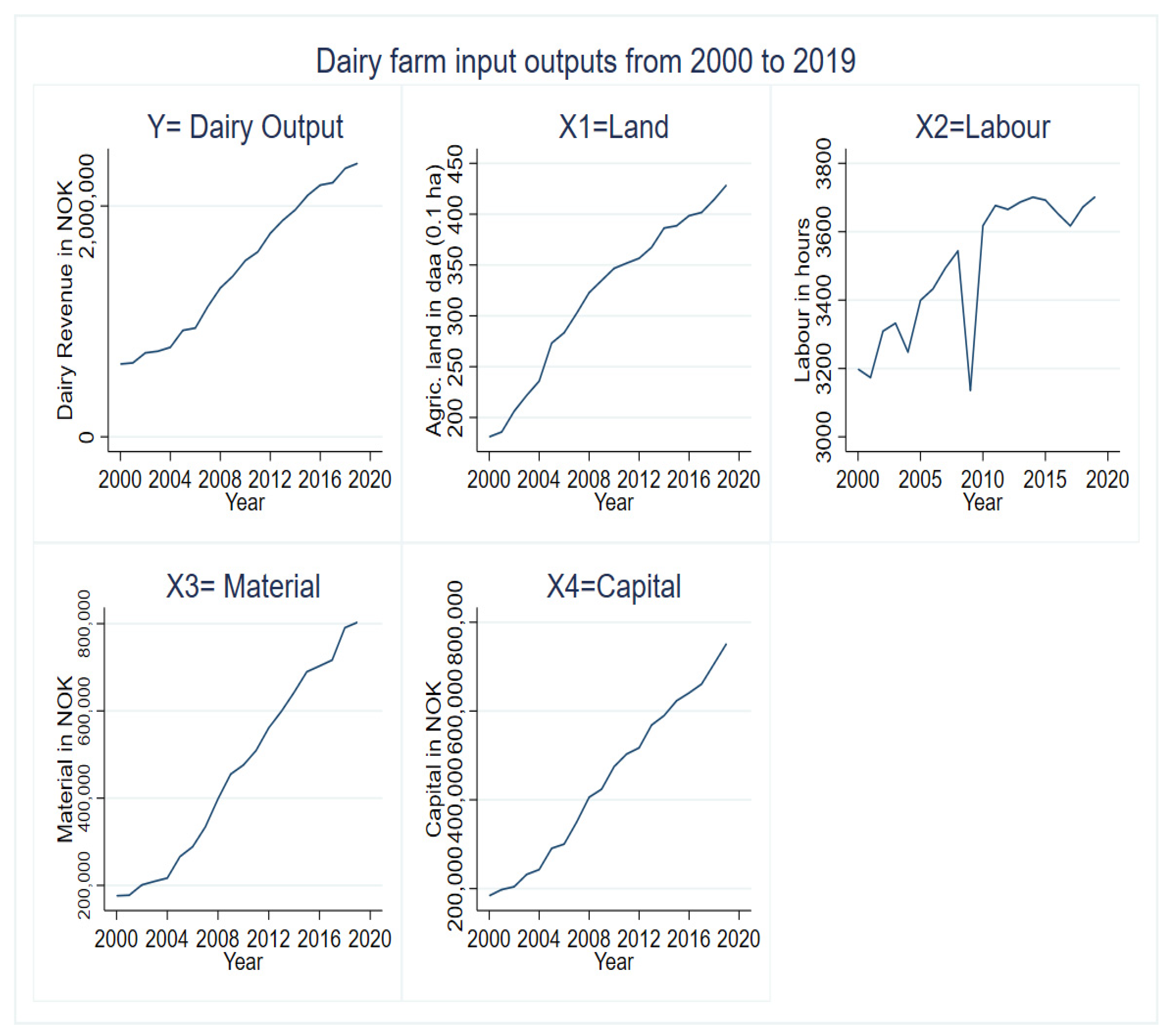
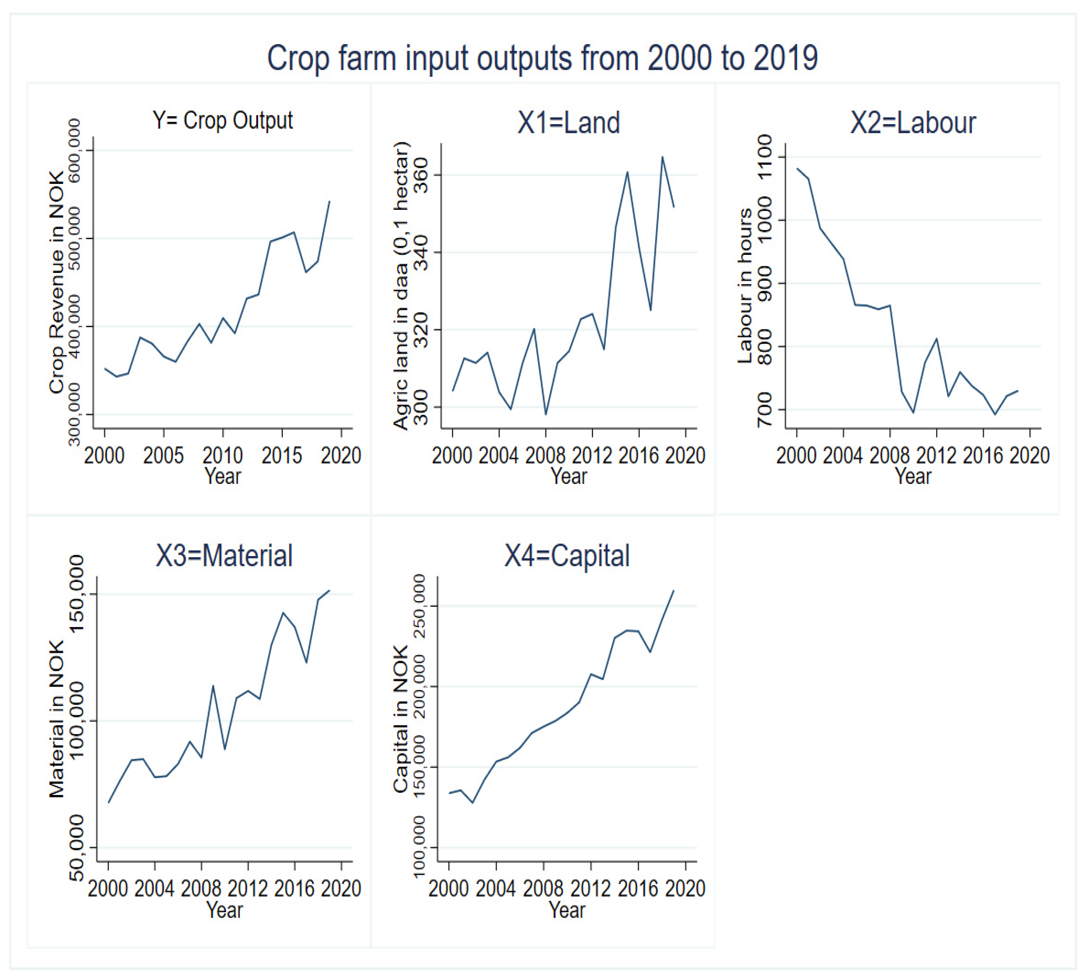
The Norwegian Institute of Bioeconomy Research provided the data used in our analysis. The analysis for the case study was based on data collected for the years 2000–2019 with a total of 5884 for dairy farms and 1880 for crop farms. Performance analysis and production technology were modeled in terms of revenue from selling the dairy and crop outputs and four inputs (land, labor, material, and capital inputs). The dairy and crop revenue are estimated in the Norwegian kroner (NOK). Land (X1) is described as the farmland calculated in hectares. The total number of hours spent working on the farm, including hired help, owners’ help, and family help, is defined as labor (X2). Fertilizers; feed; oil and fuel items; power, crop, and animal protection expenditures; building supplies; and other expenses are examples of variable inputs (X3). The expenses associated with capital inputs (X4) include both fixed-cost items and the depreciation and maintenance associated with farm capital secured by animals, buildings, and machinery. All monitoring values are expressed in NOK and are CPI-adjusted for 2019 values. We analyzed the two farming systems separately.

Table 1. Dairy and agricultural farm descriptive statistics (mean value) from 2000 to 2019.

Region	N	Output NOK *	Land (hectare)	Labor (h)	Materials NOK	Capital Inputs NOK
Dairy
Mean	5884	1,564,994	34	3534	499,085	477,652
Stand. Dev		(955,094)	(18)	(1032)	(359,437)	(300,762)
Crop
Mean	1880	489,228	35	929	117,249	196,021
Stand. Dev		(353,439)	(22)	(676)	(88,190)	(141,701)

* NOK = Norwegian Kroner and Ca. I NOK = 0.1 USD.

shows the descriptive statistics of variables used for the analysis. Figure 1 and Figure 2 show the trend of inputs and outputs for dairy and crop-producing farms. Except for labor inputs in the crop sector, both farm types of input–output levels grow over time. The decrease in labor inputs indicates that Norway’s agriculture in the crop sector is becoming increasingly capital- and technology-intensive.

5. Results and Discussion

Table 2. Dairy and crop farms’ technical efficiency score distribution.

Percentile	Technical Efficiency Dairy Farms	Technical Efficiency Crop Farms
1%	0.65	0.57
5%	0.73	0.71
10%	0.77	0.73
25%	0.82	0.78
Mean	0.85	0.82
75%	0.87	0.86
90%	0.89	0.88
95%	0.90	0.90
99%	0.92	0.91
Standard Deviation	0.05	0.06
Observation	5884	1880

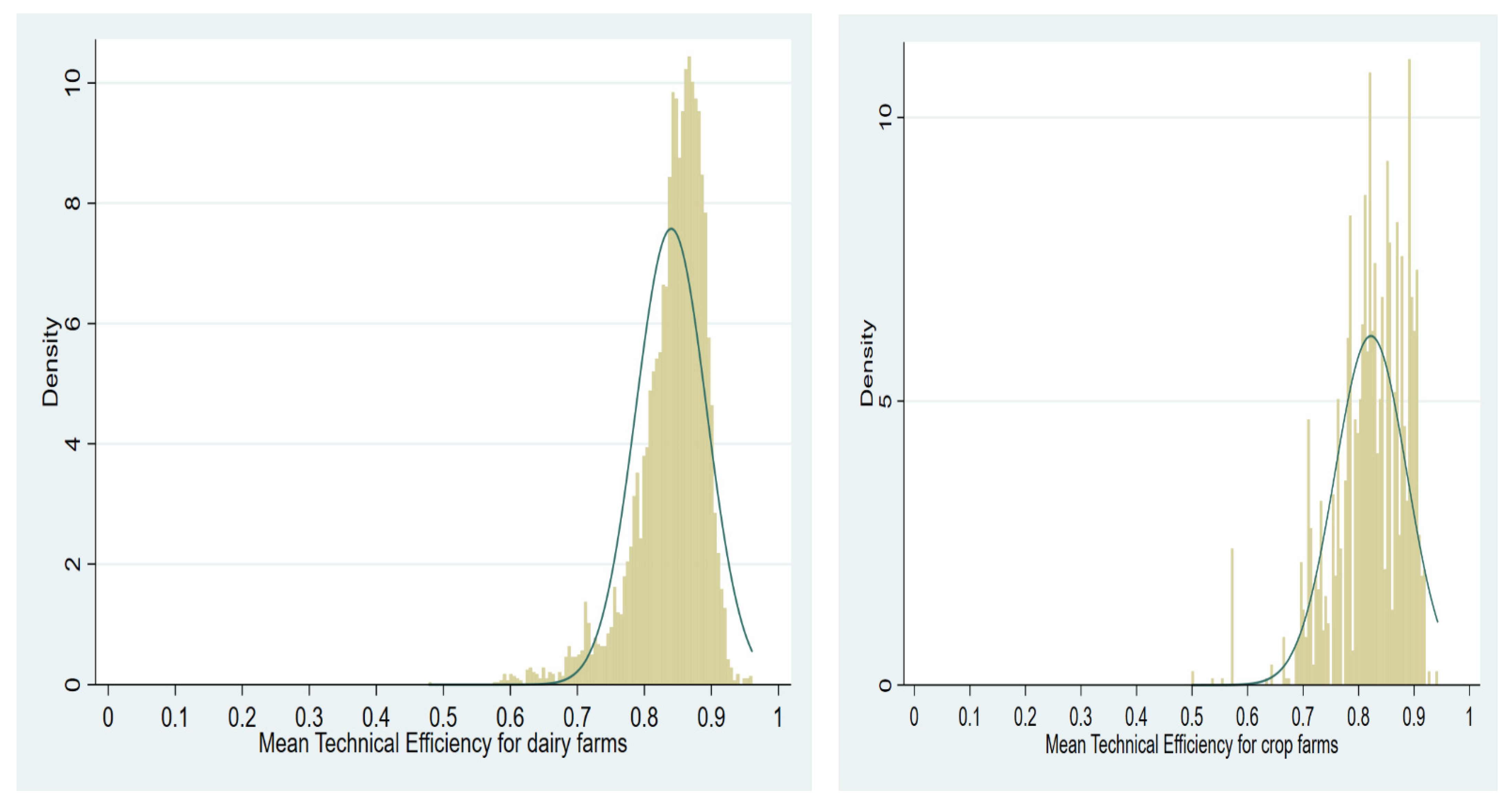
Source: Own calculation.

displays the findings for estimated technical efficiency. For most farmers, the efficiency ranges from 0.82 to 0.92. With a mean technical efficiency score of 0.85, dairy farms are generally considered to be technically inefficient. According to the efficiency rating, Norwegian dairy farms could boost output by 15% while using the same input if the process becomes technically efficient. Our results are in line with those of other studies that have been conducted in the past; for example, Alem et al. (2019) reported an average technical efficiency of 0.90% using farm-level balanced panel data from 1992 to 2014. Sipiläinen et al. (2013) reported 0.95% technical efficiency for Norwegian dairy farms from 1991 to 2008.

Estimates of the crop farms’ technical efficiency scores are shown in Table 2. The findings indicate that from 2000 to 2019, the technical efficiency was 82% on average. Additionally, Table 2 displays the distribution of the sample farms based on their technical efficiency. For example, 1% of the farms are only 57% efficient, whereas 10% of the sample farms are 73% efficient. The results suggest that there is a possibility of increasing crop production on average by 18% if all farmers are efficient enough to use the production resources. Our findings are consistent with previous research; see, for example, Lien et al. (2018), who reported 0.82% for Norwegian crop-producing farms observed from 1993 to 2014, while Alem (2020) reported mean efficiency of 92% for crop-producing farms observed from 1991 to 2013. The range of mean technical efficiency for dairy and crop farms is shown in Figure 3.

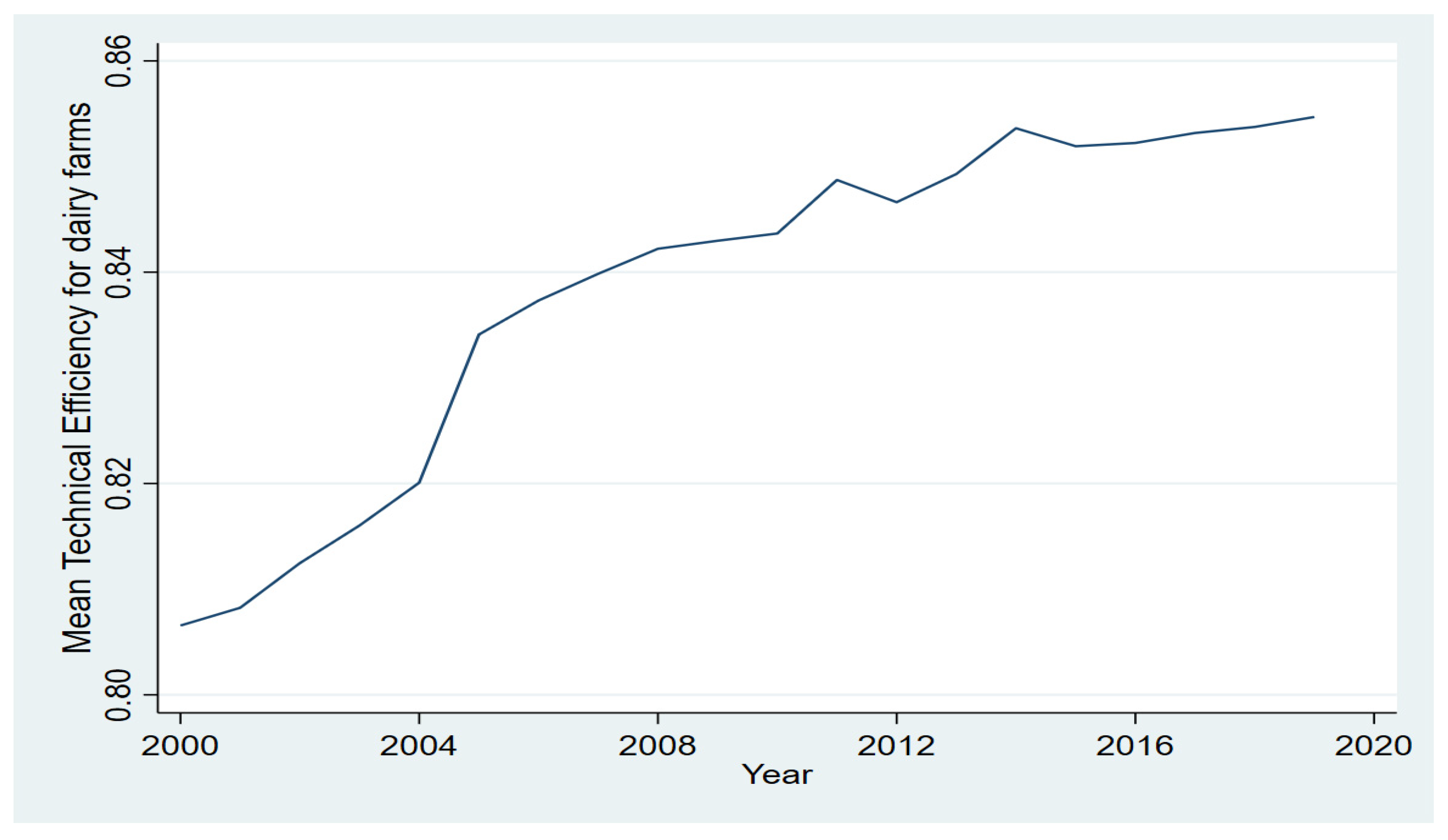
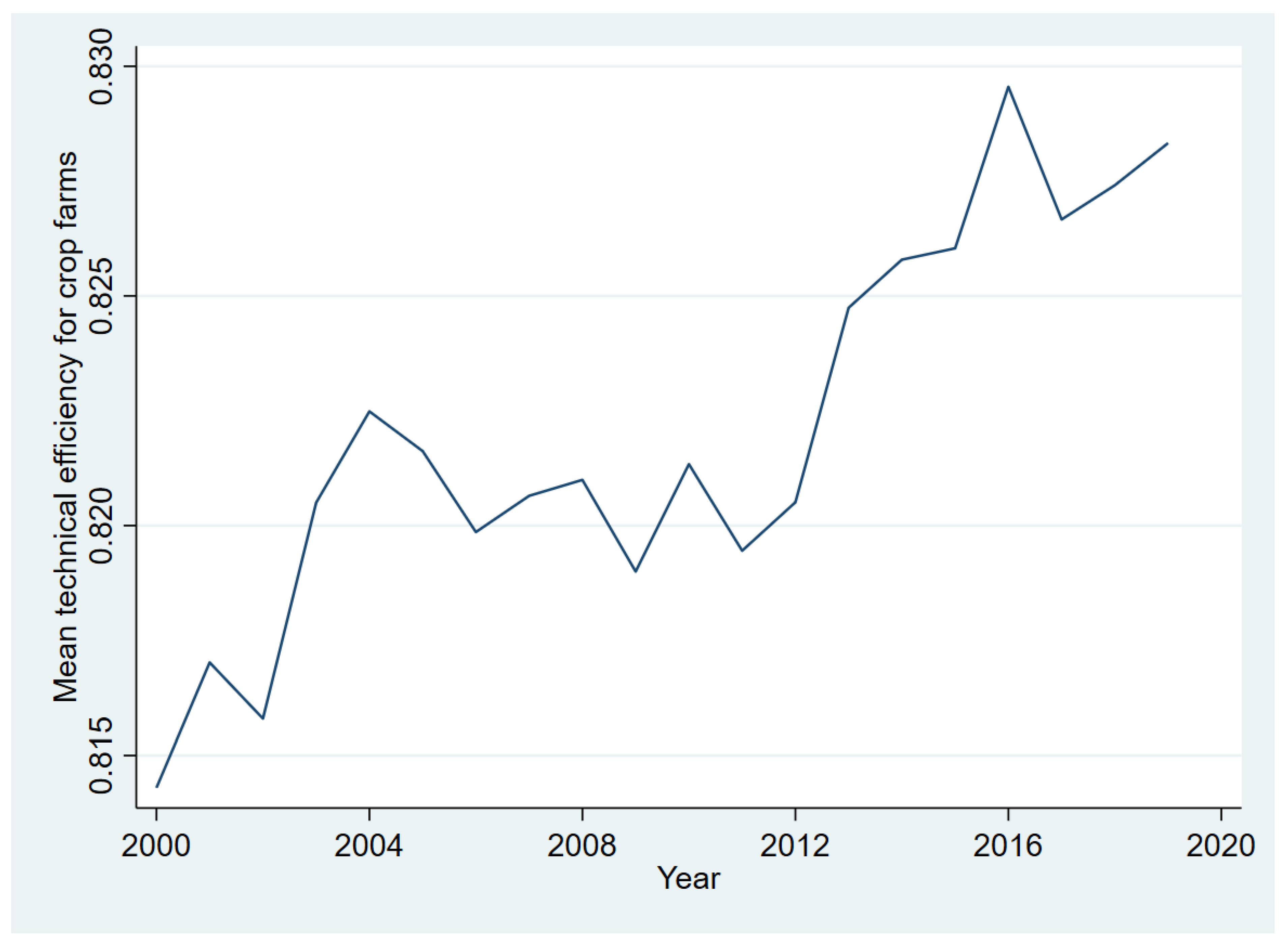
The performance of dairy farms was relatively improving over time while crop farms’ performance fluctuated over time (Figure 4 and Figure 5).

A detailed per-year efficiency score is reported in

Table 3. Mean technical efficiency scores per year for dairy and crop farms.

	Dairy Farms			Crop Farms
Year	Mean	Std. Dev.	Freq.	Mean	Std. Dev.	Freq.
2000	0.807	0.079	114	0.814	0.074	90
2001	0.808	0.077	108	0.817	0.069	92
2002	0.812	0.074	124	0.816	0.068	89
2003	0.816	0.072	126	0.820	0.068	87
2004	0.820	0.072	127	0.822	0.064	90
2005	0.834	0.064	439	0.822	0.067	89
2006	0.837	0.062	401	0.820	0.067	89
2007	0.840	0.058	398	0.821	0.062	94
2008	0.842	0.059	378	0.821	0.064	90
2009	0.843	0.059	351	0.819	0.068	97
2010	0.844	0.058	333	0.821	0.066	95
2011	0.849	0.055	344	0.819	0.066	98
2012	0.847	0.053	347	0.821	0.069	97
2013	0.849	0.054	342	0.825	0.064	92
2014	0.854	0.050	347	0.826	0.061	96
2015	0.852	0.050	335	0.826	0.062	94
2016	0.852	0.048	332	0.830	0.059	97
2017	0.853	0.048	315	0.827	0.058	99
2018	0.854	0.050	314	0.827	0.063	101
2019	0.855	0.049	309	0.828	0.063	104
Total	0.849	0.059	5884	0.822	0.064	1880

. The tables show that the mean technical efficiency value has fluctuated over the past 20 years.

6. Conclusions and Policy Implications

The study employed case studies from Norwegian agriculture to measure the performance of dairy and crop farms with farm heterogeneity control. The empirical analysis of the case study was based on data collected from 2000 to 2019, with a total of 5884 dairy farms and 1880 crop farms. The findings reveal that dairy and crop growers used suboptimal technology. According to the findings, if all farmers pursue an efficient and sustainable path, there is a chance of increasing output by 15% and 18% for crop and dairy farms, respectively. Allowing farm experience sharing, for example, allows less experienced dairy and crop-producing farms to learn from the highest-performing farms. Farmers with more years of experience are more likely to use production resources more effectively than farmers with fewer years of experience, so policy makers should encourage experience sharing to increase the efficiency of underperforming farms. The technical efficiency analysis is predicated on a static framework. The efficiency of resource use may be dynamic, which is beyond the scope of this study and should be investigated further in the future.

References

- Agrell, Per, Mehasi Farsi, and Martin Koller. 2014. Unobserved Heterogeneous Effects in the Cost Efficiency Analysis of Electricity Distribution Systems. In The Interrelationship between Financial and Energy Markets. Berlin/Heidelberg: Springer, pp. 281–302. [Google Scholar]
- Aigner, Dennis, CA Knox Lovell, and Peter Schmidt. 1977. Formulation and estimation of stochastic frontier production function models. Journal of Econometrics 6: 21–37. [Google Scholar] [CrossRef]
- Alem, Habtamu. 2018. Effects of model specification, short-run, and long-run inefficiency: An empirical analysis of stochastic frontier models. Zemedelska Economika 64: 508–16. [Google Scholar] [CrossRef]
- Alem, Habtamu. 2020. Economic performance among Norwegian crop farms accounting for farm management and socio-economic factors. International Journal of Business Performance Management 21: 417–36. [Google Scholar] [CrossRef]
- Alem, Habtamu. 2021a. A metafrontier analysis on the performance of grain-producing regions in Norway. Economies 9: 10. [Google Scholar] [CrossRef]
- Alem, Habtamu. 2021b. The Role of Technical Efficiency Achieving Sustainable Development: A Dynamic Analysis of Norwegian Dairy Farms. Sustainability 13: 1841. [Google Scholar] [CrossRef]
- Alem, Habtamu, Gudbrand Lien, and Brian Hardaker. 2018. Economic performance and efficiency determinants of crop-producing farms in Norway. International Journal of Productivity and Performance Management 67: 9. [Google Scholar] [CrossRef] [Green Version]
- Alem, Habtamu, Gudbrand Lien, Brian Hardaker, and Atle Guttormsen. 2019. Regional differences in technical efficiency and technological gap of Norwegian dairy farms: A stochastic meta-frontier model. Applied Economics 51: 409–21. [Google Scholar] [CrossRef]
- Alvarez, Antonio, Julio Corral, and Loren Tauer. 2012. Modeling unobserved heterogeneity in New York dairy farms: One-stage versus two-stage models. Agricultural and Resource Economics Review 41: 275. [Google Scholar] [CrossRef]
- Battese, George E., and Tim J. Coelli. 1992. Frontier production functions, technical efficiency and panel data: With application to paddy farmers in India. Journal of Productivity Analysis 3: 153–69. [Google Scholar] [CrossRef]
- Battese, George Edward, and Tim J. Coelli. 1995. A model for technical inefficiency effects in a stochastic frontier production function for panel data. Empirical Economics 20: 325–32. [Google Scholar] [CrossRef]
- Cornwell, Christopher, Peter Schmidt, and Robin C. Sickles. 1990. Production frontiers with cross-sectional and time-series variation in efficiency levels. Journal of Econometrics 46: 185–200. [Google Scholar] [CrossRef]
- Greene, William. 2005a. Reconsidering heterogeneity in panel data estimators of the stochastic frontier model. Journal of Econometrics 126: 269–303. [Google Scholar] [CrossRef]
- Greene, William. 2005b. Fixed and Random Effects in Stochastic Frontier Models. Journal of Productivity Analysis 23: 7–32. [Google Scholar] [CrossRef] [Green Version]
- Jondrow, James, CA Knox Lovell, Ivan S. Materov, and Peter Schmidt. 1982. On the estimation of technical inefficiency in stochastic frontier production function model. Journal of Econometrics 19: 233–38. [Google Scholar] [CrossRef] [Green Version]
- Kumbhakar, Subal C. 1990. Production frontiers, panel data, and time-varying technical inefficiency. Journal of Econometrics 46: 201–11. [Google Scholar] [CrossRef]
- Kumbhakar, Subal C., and Gudbrand Lien. 2009. Productivity and profitability decomposition: A parametric distance function approach. Food Economics—Acta Agriculturae Scandinavica, Section C 6: 143–55. [Google Scholar] [CrossRef]
- Kumbhakar, Subal C., Gudbrand Lien, and J. Brian Hardaker. 2014. Technical efficiency in competing panel data models: A study of Norwegian grain farming. Journal of Productivity Analysis 41: 321–37. [Google Scholar] [CrossRef] [Green Version]
- Kumbhakar, Subal C., Gudbrand Lien, Ola Flaten, and Ragnar Tveterås. 2008. Impacts of Norwegian milk quotas on output growth: A modified distance function approach. Journal of Agricultural Economics 59: 350–69. [Google Scholar] [CrossRef]
- Kumbhakar, Subal C., Hongren Wang, and Alen P. Horncastle. 2015. A Practitioner’s Guide to Stochastic Frontier Analysis Using Stata. Cambridge: Cambridge University Press. [Google Scholar]
- Latruffe, Laura, Ambre Diazabakana, Christian Bockstaller, Yann Desjeux, John Finn, Edel Kelly, Mary Ryan, and Sandra Uthes. 2016. Measurement of sustainability in agriculture: A review of indicators. Studies in Agricultural Economics 118: 123–30. [Google Scholar] [CrossRef]
- Lien, Gudbrand, Subal C. Kumbhakar, and Alem Habtamu. 2018. Endogeneity, heterogeneity, and determinants of inefficiency in Norwegian crop-producing farms. International Journal of Production Economics 201: 53–61. [Google Scholar] [CrossRef]
- Meeusen, Wim, and Julien van den Broeck. 1977. Efficiency Estimation from Cobb-Douglas Production Functions with Composed Error. International Economic Review 18: 435–44. [Google Scholar] [CrossRef]
- Pitt, Mark M., and Lung-Fei Lee. 1981. The measurement and sources of technical inefficiency in the Indonesian weaving industry. Journal of Development Economics 9: 43–64. [Google Scholar] [CrossRef]
- Schmidt, Peter, and Robin C. Sickles. 1984. Production frontiers and panel data. Journal of Business & Economic Statistics 2: 367–74. [Google Scholar]
- Sipiläinen, Timo, Subal C. Kumbhakar, and Gudbrand Lien. 2013. Performance of dairy farms in Finland and Norway for 1991–2008. European Review of Agricultural Economics 41: 63–86. [Google Scholar] [CrossRef]
- SSB. 2021. Agriculture, Forestry, Hunting, and Fishing. Available online: https://www.ssb.no/en/jord-skog-jakt-og-fiskeri/jordbruk (accessed on 24 October 2022).
Figure 1.
Dairy farm inputs and output (revenue) for the years 2000–2019.
Figure 2.
Crop farm inputs and output (revenue) for the years 2000–2019.
Figure 3.
Dairy and crop farms’ technical efficiency score distribution.
Figure 4.
Dairy farms’ technical efficiency score distribution.
Figure 5.
Crop farms’ technical efficiency score distribution.