
Resilience of an Urban Coastal Ecosystem in the Caribbean: A Remote Sensing Approach in Western Puerto Rico


1
Department of Agro-Environmental Sciences, Mayagüez Campus, University of Puerto Rico, Mayagüez, PR 00680, USA
2
Department of Agricultural and Biosystems Engineering, Mayagüez Campus, University of Puerto Rico, Mayagüez, PR 00680, USA
*
Author to whom correspondence should be addressed.
Earth 2024, 5(1), 72-89; https://doi.org/10.3390/earth5010004
Submission received: 31 December 2023
/
Revised: 1 February 2024
/
Accepted: 8 February 2024
/
Published: 10 February 2024
Abstract
:Utilization of remote sensing-derived meteorological data is a valuable alternative for tropical insular territories such as Puerto Rico (PR). The study of ecosystem resilience in insular territories is an underdeveloped area of investigation. Little research has focused on studying how an ecosystem in PR responds to and recovers from unique meteorological events (e.g., hurricanes). This work aims to investigate how an ecosystem in Western Puerto Rico responds to extreme climate events and fluctuations, with a specific focus on evaluating its innate resilience. The Antillean islands in the Caribbean and Atlantic are vulnerable to intense weather phenomena, such as hurricanes. Due to the distinct tropical conditions inherent to this region, and the ongoing urban development of coastal areas, their ecosystems are constantly affected. Key indicators, including gross primary production (GPP), normalized difference vegetation index (NDVI), actual evapotranspiration (ET), and land surface temperature (LST), are examined to comprehend the interplay between these factors within the context of the Culebrinas River Watershed (CRW) ecosystem over the past decade during the peak of hurricane season. Data processing and analyses were performed on datasets provided by Moderate Resolution Imaging Spectroradiometer (MODIS) and Landsat 8–9 OLI TRIS, supplemented by information sourced from Puerto Rico Water and Energy Balance (PRWEB)—a dataset derived from Geostationary Operational Environmental Satellite (GOES) data. The findings revealed a complex interrelationship among atmospheric events and anthropogenic activities within the CRW, a region prone to recurrent atmospheric disruptions. NDVI and ET values from 2015 to 2019 showed the ecosystem’s capacity to recover after a prolonged drought period (2015) and Hurricanes Irma and Maria (2017). In 2015, the NDVI average was 0.79; after Hurricanes Irma and Maria in 2017, the NDVI dropped to 0.6, while in 2019, it had already increased to 0.8. Similarly, average ET values went from 3.2339 kg/m2/day in 2017 to 2.6513 kg/m2/day in 2018. Meanwhile, by 2019, the average ET was estimated to be 3.8105 kg/m2/day. Data geoprocessing of LST, NDVI, GPP, and ET, coupled with correlation analyses, revealed positive correlations among ET, NDVI, and GPP. Our results showed that areas with little anthropogenic impact displayed a more rapid and resilient restoration of the ecosystem. The spatial distribution of vegetation and impervious surfaces further highlights that areas closer to mountains have shown higher resilience while urban coastal areas have faced greater challenges in recovering from atmospheric events, thus showing the importance of preserving native vegetation, particularly mangroves, for long-term ecosystem stability. This study contributes to a deeper understanding of the dynamic interactions within urban coastal ecosystems in insular territories, emphasizing their resilience in the context of both natural atmospheric events and human activity. The insights gained from this research offer valuable guidance for managing and safeguarding ecosystems in similar regions characterized by their susceptibility to extreme weather phenomena.
1. Introduction
Puerto Rico (PR) is a tropical island in the Caribbean that commonly experiences atmospheric events that impact its ecosystems and hydrological cycle; they are designated as 10-, 50-, and 100-year events. The timeframe between Hurricanes Irma and Maria in 2017 and Hurricane Fiona in 2022 indicates that these 10-, 50-, and 100-year events are happening more frequently than normally estimated. Therefore, tools that can help us understand ecosystem resilience, using remotely sensed temporal and spatial data, are needed to manage these challenges caused by extreme weather events. Although PR has a vast amount of meteorological or atmospheric data, other insular territories (e.g., Haiti, Dominican Republic) have limited or null meteorological data measured in situ. Therefore, the use of remote sensing meteorological and atmospheric data can be an alternative method to compensate for a lack of readily available datasets.
Remote sensing data can help determine ecosystem health through metabolism or productivity assessment and by observing interactions between other system components [1,2]. Products such as Landsat 8–9 and Moderate Resolution Image Spectroradiometer (MODIS) are good alternative tools that can produce high-resolution images at a regional and national scale. For example, MOD16A is based on the Penman-Monteith equation, which contains daily meteorological data along with MODIS data such as vegetation dynamics, albedo (fraction of light that a surface reflects), and land cover. Most MODIS bands have a spatial resolution of 1 km, where each pixel would represent an area of 1 × 1 km2. Moreover, these products usually have a radiometer resolution of 16-bit depth.
Precipitation, evapotranspiration (ET), and runoff are the major water fluxes considered in the hydrologic cycle, which comprises atmospheric water and land water (rivers, lakes, and groundwater) [3]. ET values consider the water that is released into the atmosphere via evaporation and transpiration, and it is a function of solar radiation, temperature, wind, and soil moisture. Climate change has affected the water cycle due to increased temperatures [4,5]. Thus, ET values are a sensitive measure to help us better understand the water cycle and the resilience of ecosystems [6,7]. Surface temperature is also a measure that can provide us with valuable information regarding the influence of the exchange of water between the atmosphere and the soil surface under extreme hydrological events [8].
ET represents vegetation’s water loss via its vascular system and evaporation from Earth’s surface. Examination of ET helps to determine the amount of water lost that needs to be replaced either by irrigation or rainfall. ET can also be used to estimate the water requirement by crops and plants in an ecosystem, thus making irrigation practices more efficient for precision agriculture [9]. Due to the impact of global climate change and extensive human activities, the study of ET and its dynamics is important in elucidating regional water cycle processes, optimizing water resource allocation, and assessing the water resources necessary for ecological development and sustainable socioeconomic progress [6,7,9]. Direct measurements to estimate ET are feasible through various instruments, such as evapotranspiration meters, vorticity correlators, and large-aperture scintillators, spanning scales from meters to kilometers [10]. However, capturing the spatiotemporal dynamics of ET at the regional scale remains challenging due to limited field observations. The integration of remote sensing techniques, climate models, and land surface models into ET numerical simulations has led to the development of diverse global and regional ET products [11,12]. These products can be categorized into three primary groups based on their method of estimation: (a) interpolation using field measurements and machine learning techniques [13]; (b) simulation through remotely sensed ET models, such as MODIS [14], and (c) reanalysis data and products assimilated using various land surface models [15]. This integration of advanced technologies and modeling approaches enhances our ability to understand and quantify ET dynamics across different spatial and temporal scales.
A study regarding ET estimation was conducted in Puerto Rico. Geostationary Operational Environmental Satellite-Puerto Rico Water and Energy Balance (GOES-PRWEB) is a product with a 1 km image resolution that provides us with additional data on actual ET estimation [15]. GOES-PRWEB is also based on the Penman-Monteith (PM) equation. Moreover, it can be used to validate data provided by MOD16A2, which is also based on Penman-Monteith. The MOD16A2 product is an 8-day product, and GOES-PRWEB has daily, monthly, and annual data. Furthermore, additional calculations are necessary to be able to compare data sets. GOES-PRWEB’s previous study suggested that ET values were underestimated [15]. Another study in Northeastern Brazil—a tropical region as well– used remote sensing technology to assess land degradation and drought impacts over terrestrial ecosystems based on water and carbon fluxes, i.e., MOD16A2 and MOD17A2 to estimate ET and gross primary production (GPP), respectively [16]. The authors reported changes resulting from human activity, which caused environmental degradation associated with drought impact.
The study of the hydrological cycle using satellite imagery is an underdeveloped area of investigation in PR. Moreover, due to a lack of research regarding gross primary production associated with ecosystem resilience in insular territories in the Caribbean, this work aims to investigate how an ecosystem in Western Puerto Rico responds to extreme climate events and fluctuations, with a specific focus on evaluating its innate resilience during peak hurricane season in a 10-year span using remotely sensed datasets. Our hypothesis is that areas with little or null anthropogenic activity show more resilience to extreme atmospheric events.
2. Materials and Methods
2.1. Study Area
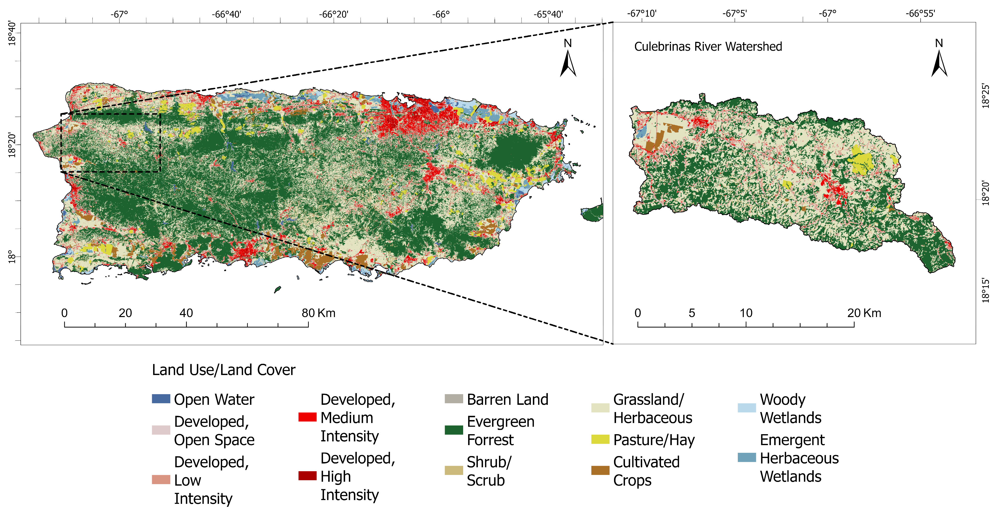
The study area is located in Western PR. It is an urban coastal exoreic watershed whose main river in its drainage network is Culebrinas. The Culebrinas River Watershed (CRW) presents various classes of land use/land cover, which makes it an adequate study area to assess the resilience of an urban coastal ecosystem (Figure 1).
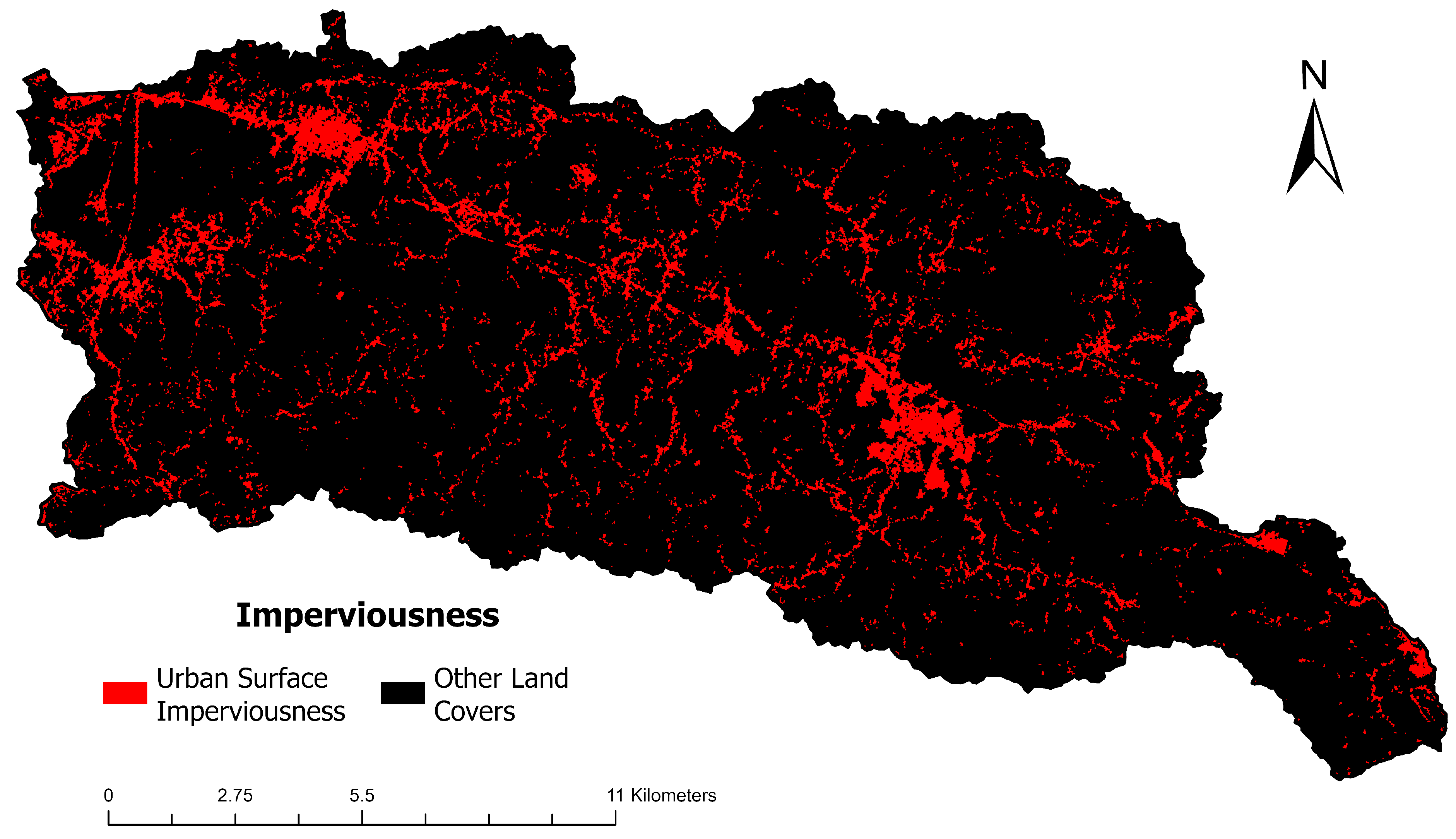
Within the CRW, there are four highly developed urban areas (Aguadilla, Aguada, Moca, and San Sebastian), which can be identified in an imperviousness map (Figure 2). Due to PR’s topography (an elevated center and low coastlines), climate classification (Af and Am in Köppen-Geiger classification) [17], and geographical location in the Atlantic Ocean, PR is prone to landslides and floods during the wet season. Urban coastal areas in PR are close to alluvial landforms and are classified as flood risk areas [18]. The results of a study that assessed agricultural activity in PR from 2012 to 2018, after the effects of major atmospheric events, showed that Hurricanes Irma and Maria (2017) destroyed many agricultural fields, which affected the agricultural sector, particularly small farms of local producers [19].
2.2. Reference Parameters and Datasets
To achieve the work’s objectives, we evaluated evapotranspiration (ET), land surface temperature (LST), normalized difference vegetation index (NDVI), and gross primary production (GGP) using remote sensing datasets from 2012 to 2021. ArcGIS was used to perform most of the geoprocessing; however, data analysis was also performed using RStudio. Attribute tables for each map were created to build correlation graphs, and each table was created as a spreadsheet using the coordinates of the datapoints within the study area for it to be compatible with RStudio. Spreadsheets were created using latitude and longitude coordinates along with datapoints (approximately 2500 points). We then used the Create Fishnet function on ArcMap to place/plot the datapoints onto the study area. Then, the values of the points were extracted using the Extract Multi Values to Points tool. For each attribute table, we used a 50 × 50 fishnet. When “clipped” to the study area, a total of approximately 1349 points was used. For a more accurate estimation of ET and LST values, adequate attribute tables were built, as gaps within these datasets had to be amended using other sources that over- or underestimated values.
To estimate the resilience of the ecosystem to atmospheric events, we compared and correlated the estimations for ET, NDVI, LST, and GPP, calculated from Landsat and MODIS. We used Landsat 8–9 OLI TRIS for LST, and MODIS products were used for ET, GPP, and NDVI. To compare the data from MODIS products, multiday values were modified into daily values. Gap-filled GPP maps were converted from an 8-day composite to daily values, and the same process was performed for MOD16A2 for ET estimations. The coordinate system for MODIS products is undefined; therefore, we defined the coordinate system using WGS 1984 UTM Zone 20N.
To calculate ET, we used MOD16A2 at a 500 m, 16-bit spatial resolution [20]. It has a valid range from −3276.1 to 3276.7:
where MOD16A-ET represents the values obtained from MODIS products for ET estimations. The 0.1 is a scale factor provided by the Land Processes Distributed Active Archive Center (LP DAAC) for ET estimations. To obtain the daily values of ET, we converted the datasets from an 8-day composite to daily ET estimations. During atmospheric events, heavily clouded zones formed in our area of study, generating uncertainty within the datasets. For ET estimations, we used GOES-PR data to amend the MOD16A2 datasets. The unit kg/m2/day is equivalent to mm/day. Thus, MODIS-derived ET is comparable/compatible with GOES-PR data. As GOES-PR has a 1 km resolution, the points plotted from GOES-PR did not fully cover the gaps. Thus, we used inverse distance weighted interpolation (IDW) to finalize amending the zones with cloud interference. IDW is a deterministic spatial interpolation that assumes that the closer the value of the interpolation is to the initial point, the more accurate it is. In general, the interpolated values from GOES-PR underestimated ET values as compared with the values obtained from MOD16A2.
ET = MOD16A2-ET * 0.1
Reddy and Manikiam [21] presented a procedure to estimate LST from Landsat 8–9 using emissivity estimation (Equation (8)). Emissivity estimations for temperature generate a grade of uncertainty to the final LST estimation, and as per Vanhellmont [22], emissivity estimations from Landsat 8–9 present good estimations for LST. For this procedure, Band 10 was used to determine brightness temperature, and Bands 4 and 5 were used for the NDVI. Other values were taken from the metadata of the maps (Table 1).
The spectral radiance was calculated as follows:
where Lmax is the maximum radiance (), Lmin is the minimum radiance (), Qcal is the value of the pixel, Qcalmax is the maximum value of pixels, Qcalmin is the minimum value of pixels, and Oi is the correction value for Band 10. These values can be obtained from the metadata file of each raster. The metadata values were the same for all years. Another method is to determine the top of the atmosphere, where is the band-specific multiplicative rescaling factor from metadata, and is the band-specific additive rescaling factor from metadata (Table 1).
The brightness temperature conversion (From Ly to BT) was then calculated as follows:
where K1 and K2 are the thermal constants of Band 10. These values can be obtained from the metadata file attached to the raster. L is the result of Equation (1). To obtain the results in Celsius, we must then subtract 273.15.
To calculate NDVI, we used two methods: (1) MOD13Q1 (16 days) at a 250 m spatial resolution and a valid range from −2 to 10, in which we applied a 0.0001 scale factor as recommended by LP DAAC [23], and (2) using Landsat 8–9 OLI with Bands 6 and 4:
where NIR is the near-infrared band value of a pixel (Band 6), and RED is the red band value of the same pixel (Band 4). It was noticed that NDVI estimates from Landsat were lower than NDVI values obtained from MODIS.
NDVI = MOD13Q1-NDVI * 0.0001
Proportional vegetation (Pv) was computed as follows:
where NDVImin is the minimum value and NDVImax is the maximum value of NDVI obtained by either Equation (5) or Equation (6). On a global scale, it is proposed to use values of NVDImin = 0.2 and NVDImax = 0.5, but in some cases, these values tend to underestimate NVDI min and max values. Due to the variation between global regions, we used the NDVI range for each year.
Land surface emissivity (LSE) was then calculated:
where λ is the average wavelength of Band 10 equal to 0.00115; and ρ is equal to 1.4388 × 10⁻² mK, which derives from (ρ = h * c/σ), where h is Planck’s constant, c is the velocity of light, and σ is the Boltzmann constant. BT and E are the results of steps 2 and 5, respectively. The result of LST (Equation (8)) is given in Celsius. Cloud corrections were made for most of the LST maps, and heavily clouded areas were erased and replaced using other daily data maps from Landsat 8–9 OLI TRIS with similar conditions to obtain . To correct these maps, we used the following condition, in which the clouds and land were represented as values of 0 and 1, respectively:
where LST is the raster name of the previously calculated raster (Equation (8)), and MaxCloud is the maximum value that represents the clouds in the LST raster. We then multiplied the condition by the original LST raster to obtain the values of clouds as zeros. After the clouds were 0, we copied the raster and assigned 0 as a NoData value. To obtain a complete map with the cloud correction, we searched for maps of the same year without clouds in the desired area. We estimated LST with additional datasets from another day within the year and evaluated to create a full raster by merging the corrected dataset with another dataset from a different day.
Con(“LST” <= MaxCloud, 0, 1)
Finally, GPP was computed as follows:
where MOD17A2 represents the values obtained from MODIS products for GPP estimations. The 0.0001 is a scale factor provided by the LP DAAC for GPP estimations [24].
GPP = MOD17A2 * 0.0001
3. Results
The results of this work reveal significant insights into how the CRW was affected by different meteorological phenomena during the timespan of the datasets. These findings are discussed in Section 4.
Table 2 presents a general overview of what occurred at the CRW from a large point of view. However, these should not be considered as average values. For example, the years 2020 and 2017 are relatively close in terms of the highest values of ET, but on a full scale, it is known that the average ET value for 2020 is greater than that for 2017.
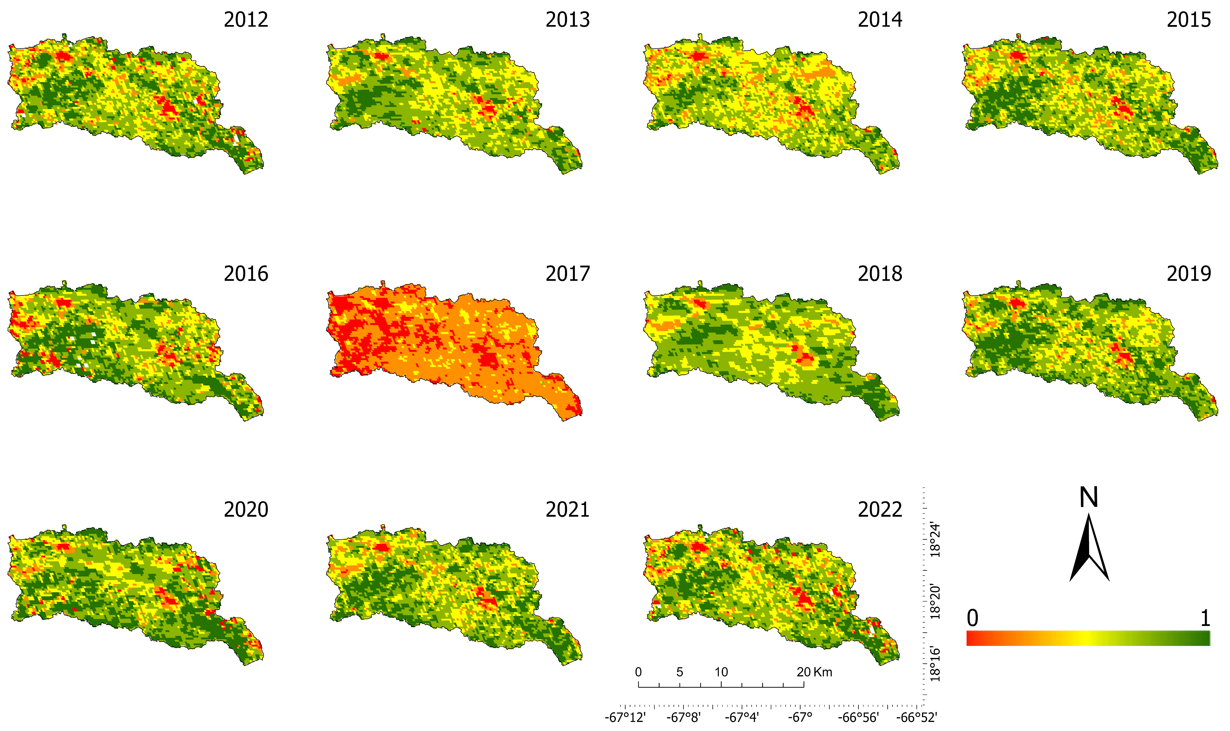
Figure 3 shows NDVI 16-day interval data. NDVI 16-day values were greater in comparison with daily NDVI values. Daily values of NDVI were calculated using Landsat 8–9 OLI-TRIS with the near-infrared band and red band.
NDVI datasets for a decade will help us estimate the health and changes in land use for Culebrinas ecosystems. These datasets help determine plant health across the watershed, and we can use these parameters to determine the resilience of ecosystems within the CRW. We also compared NDVI with the other evaluated parameters during the time of study. NDVI values for 2017 were the lowest values of NDVI for the decade evaluated. Hurricane Maria’s strong winds, floods, and landslides also had a negative effect on the vegetation in Puerto Rico. The biggest impact on health and vegetation cover for 2017 was seen in regions closer to the coast or urban areas where the ecosystem was already weakened.
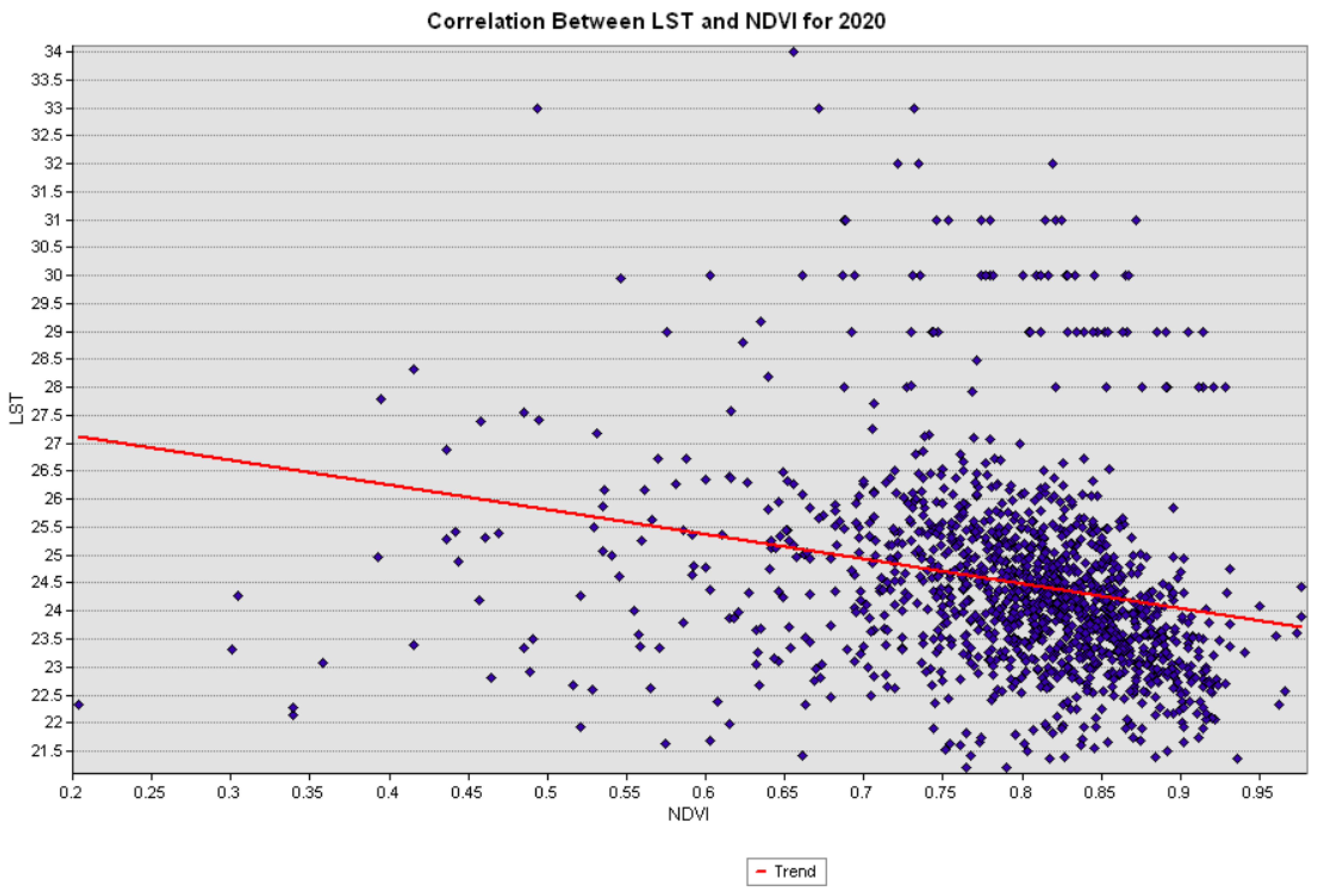
Coastal areas are more prone to significant changes in vegetation after a hurricane, due to the type/amount of vegetation. The type of vegetation closer to the coast is mainly grassland, whereas in the mountain range, we can find forest areas with denser vegetation. Because of the density of the vegetation in the mountain range, loss of vegetation is less prone to happen. Additionally, 16-day NDVI values from MODIS have a pixel resolution of 250 m and have been available since 2000 to present. We can use values of NDVI to see trends and the effect that atmospheric events have on vegetation cover. For example, as shown in Figure 3, the trend for 2020 was that greater values of NDVI were present at lower temperatures. Lastly, the map of September 2022 shows NDVI values during a prolonged dry season in Puerto Rico. This is associated with the correlation of LST and NDVI (Figure 4).
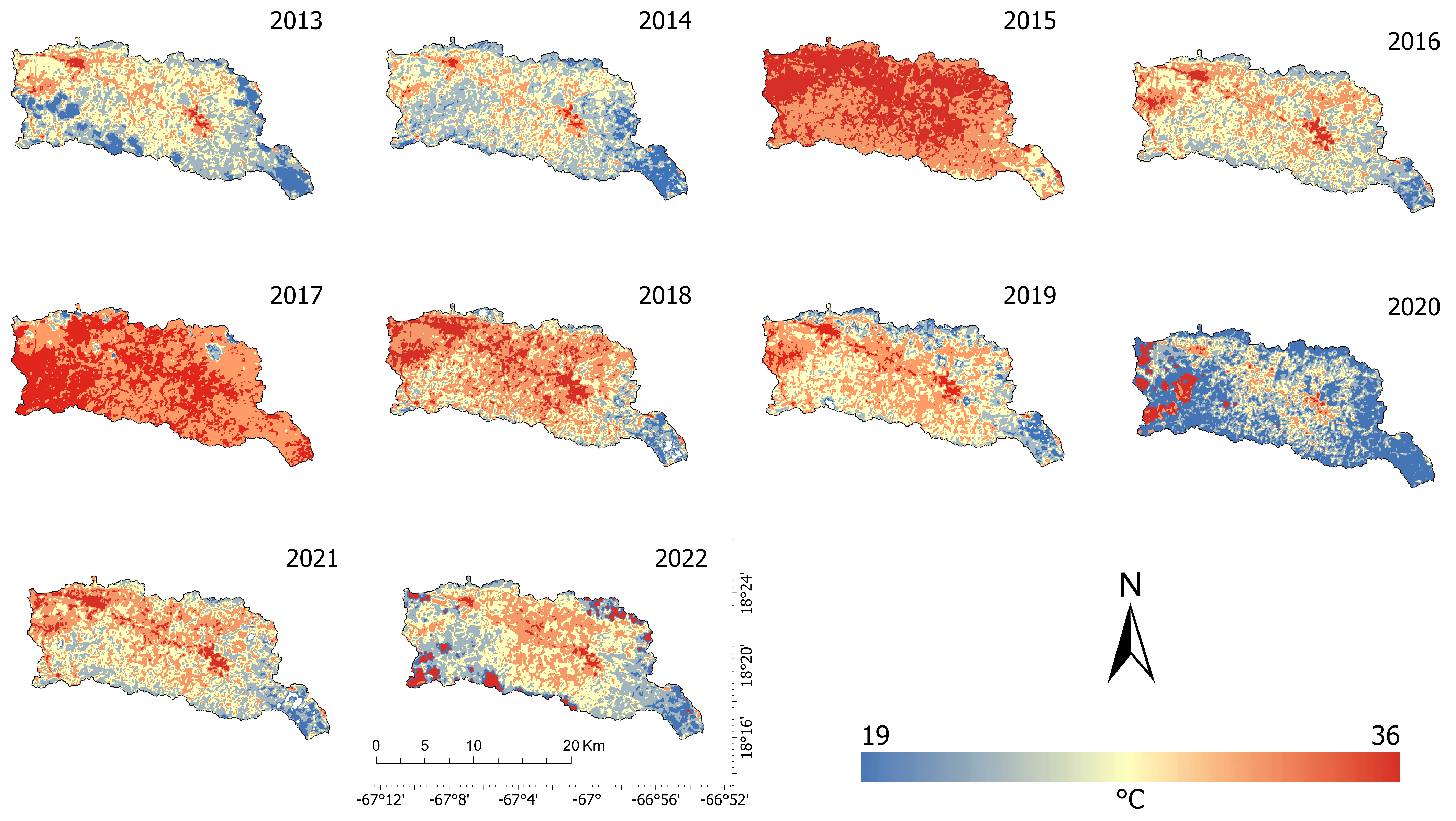
The LST estimates were computed using Landsat 8–9 datasets. As Landsat 8 was launched on an Atlas-V rocket in February 2013, there are no available data before 2013. Landsat 8–9 is a 30 m resolution image. Figure 5 shows the spatial distribution for LST within the CRW. In 2015 and 2017, LST had the highest values out of all the years studied, yet in 2015, there was an extreme drought. Additionally, in 2017, Hurricane Maria caused bare land or a major lack of vegetation.
Land surface temperature presented high values in 2017 after Hurricane Maria due to the lack of vegetation. This agrees with a study presented by Villalobos [25], where it is mentioned that soil that is exposed to radiation reflects part of it and retains the rest, which increases the soil’s temperature. This would also be the case for 2015, but it remained this way for a longer period due to a lack of water. For 2020, there is some discrepancy between data from September 28 and the data used to substitute clouds, which were taken from October to November.
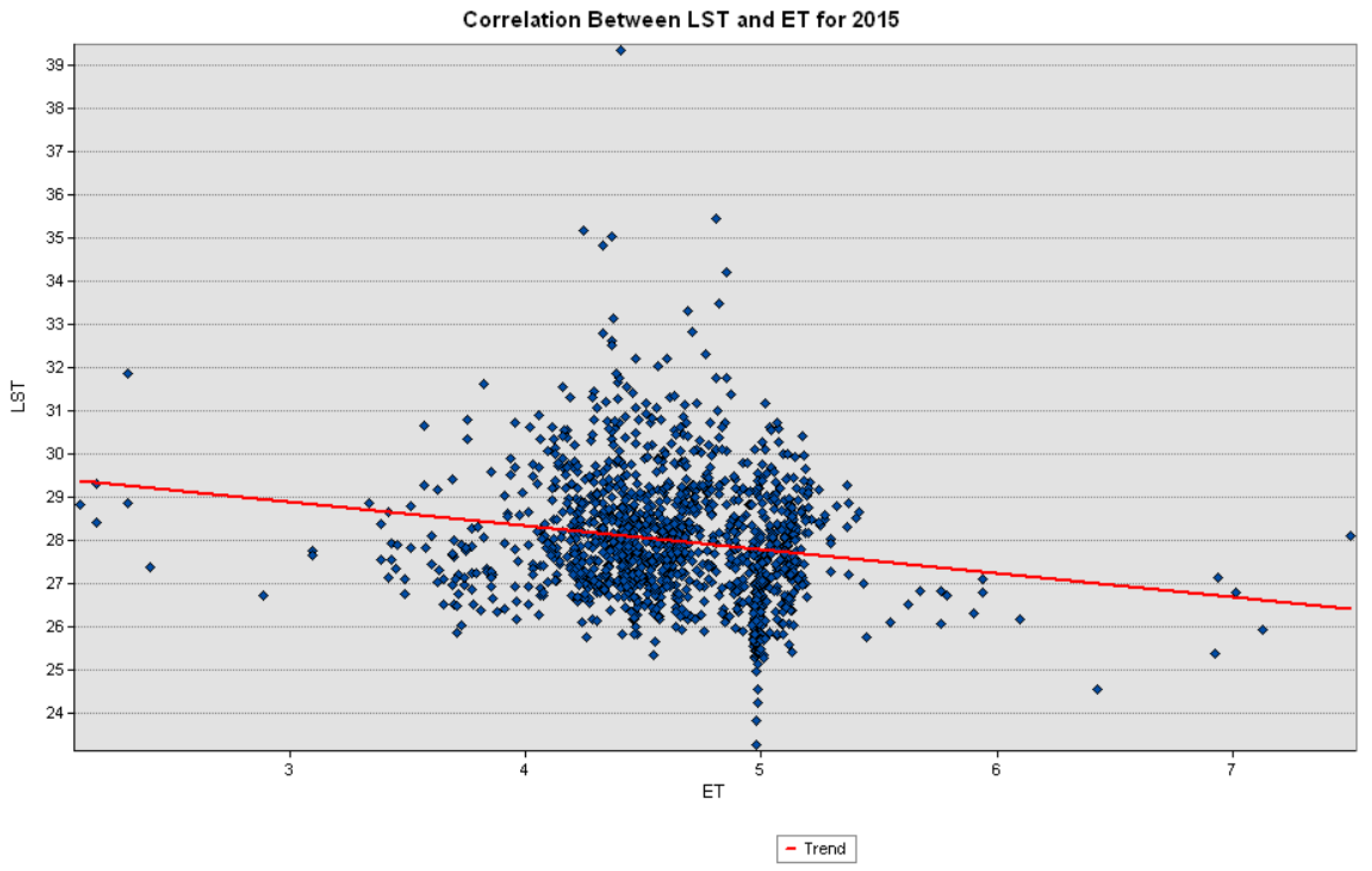
LST and ET daily values are compared on the scatterplot graph in Figure 6. In this case, as daily data are being observed, the correlation is not as clear as in the previous one. Nevertheless, it is suggested that, on that day, most of the evapotranspiration occurred at higher temperatures. At higher temperatures, it is usually noted that plants will transpire more, and a greater amount of water will evaporate. These standards may have not applied in 2015 because it is noted that ET, NDVI, and GPP are more responsive to precipitation, which was null during this timeframe.
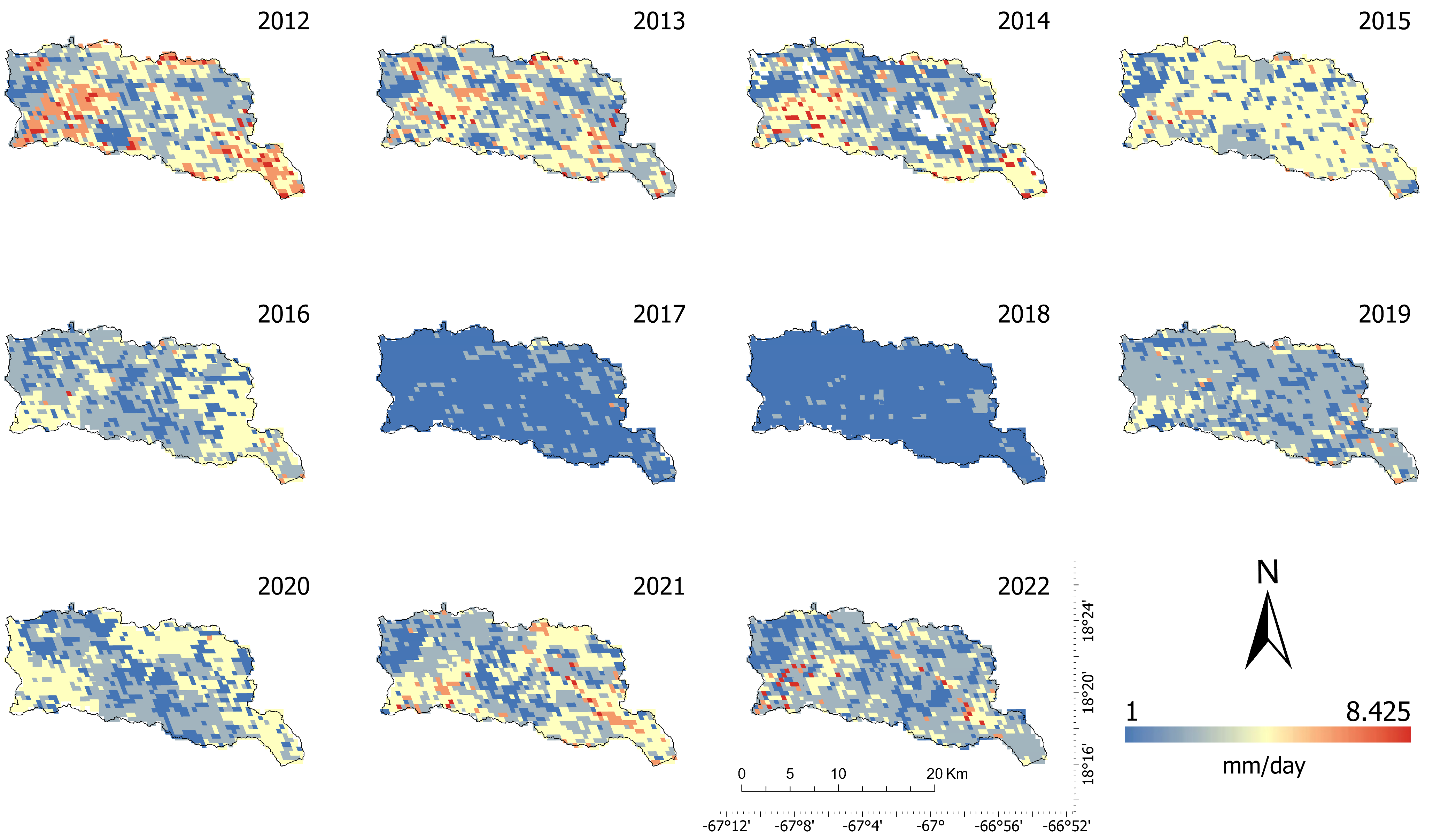
MOD16A2 products have fill values. These are values from 32,761 through 32,767, and it is recommended they are disregarded. When excluding these values, the data sets from 2015 to 2022 lost most of their data. Therefore, lost data had to be replaced for this study. To accomplish this, we used data values from 2012 to 2022 from GOES-PRWEB. From each dataset, 85 points were extracted and integrated into our MOD16A2 raster. We then proceeded to complete the MODIS products’ missing information (Figure 7) using inverse distance weighted interpolation (IDW).
IDW interpolation from GOES-PR underestimated the values of actual ET in comparison with that obtained from MODIS. It is to be considered that the points further away from the interpolated data will not be as reliable as the points closer to the fishnet points. Therefore, values obtained from GOES-PR were not used to create correlation graphs or matrices.
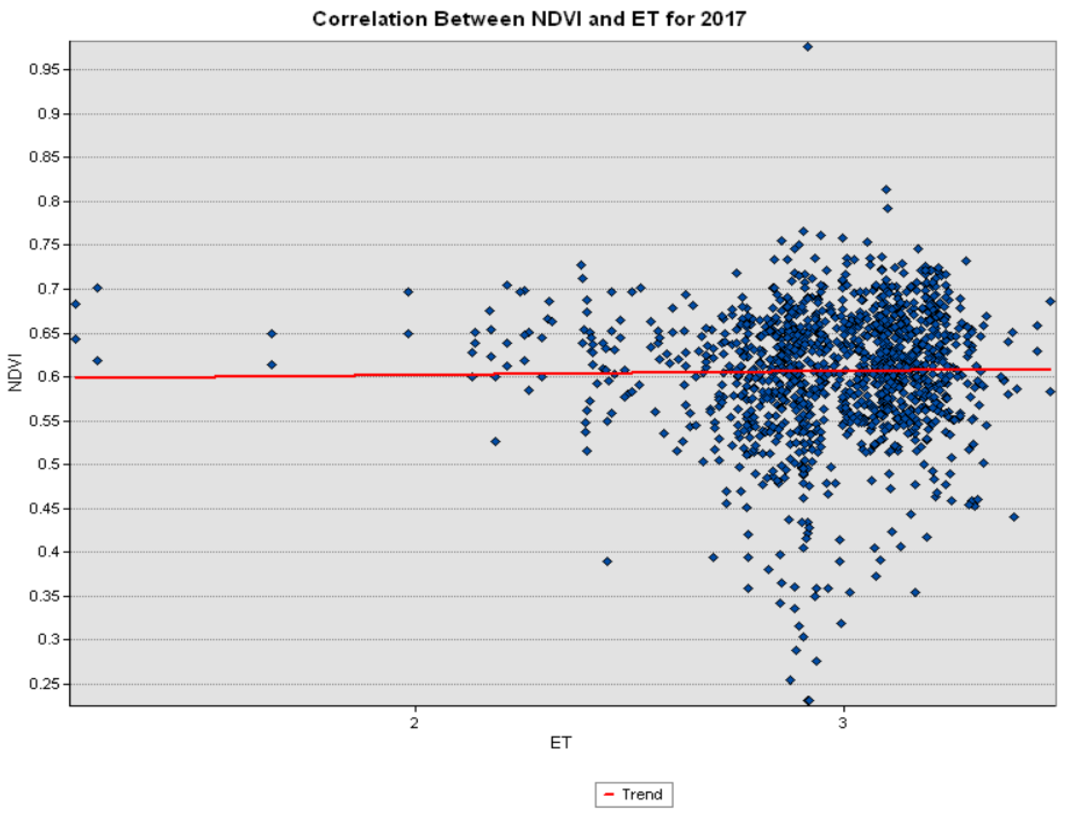
Evapotranspiration is directly related to plant maturity and amount. Therefore, it is expected that an increase in ET will be related to an increase in NDVI values (Figure 8). Compared with other years, in 2017, ET and NDVI were at their lowest values due to Hurricane Maria. Although NDVI responds well to moderate or extreme wet events, Hurricane Maria’s main impact on the island was from its strong winds. Nevertheless, the trend between 2017 and other years tends to be the same, where an increase in NDVI will cause an increase in ET, and vice versa.
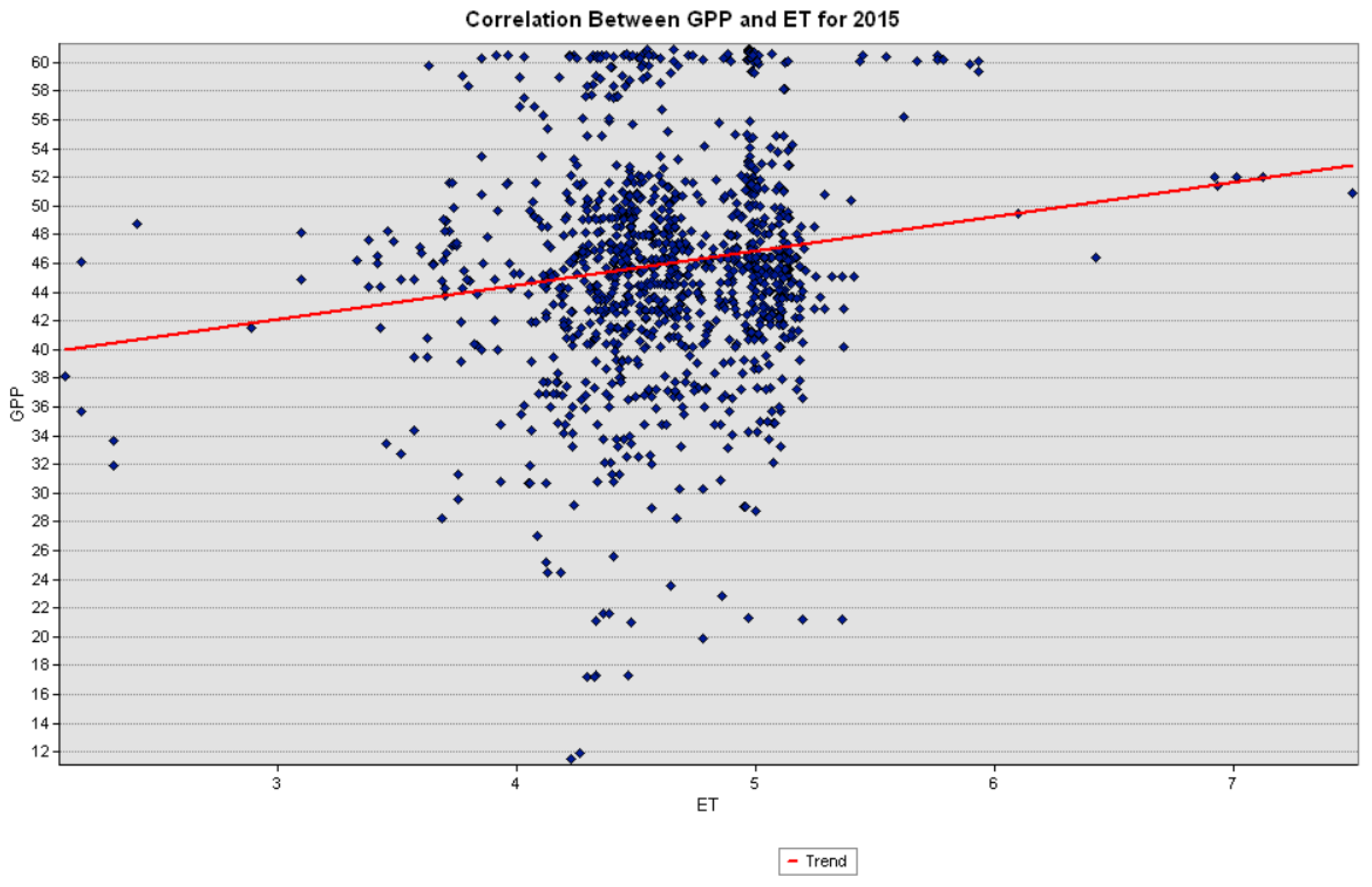
In Figure 9, the correlation between GPP and ET is positive. A positive trend means that an increase in GPP will produce an increase in ET, and vice versa. For GPP, production values of 3276.19 g/C/day were not taken into consideration, as these values are nonterrestrial fill value classes. In this case, these values’ land cover was assigned as urban/built-up.
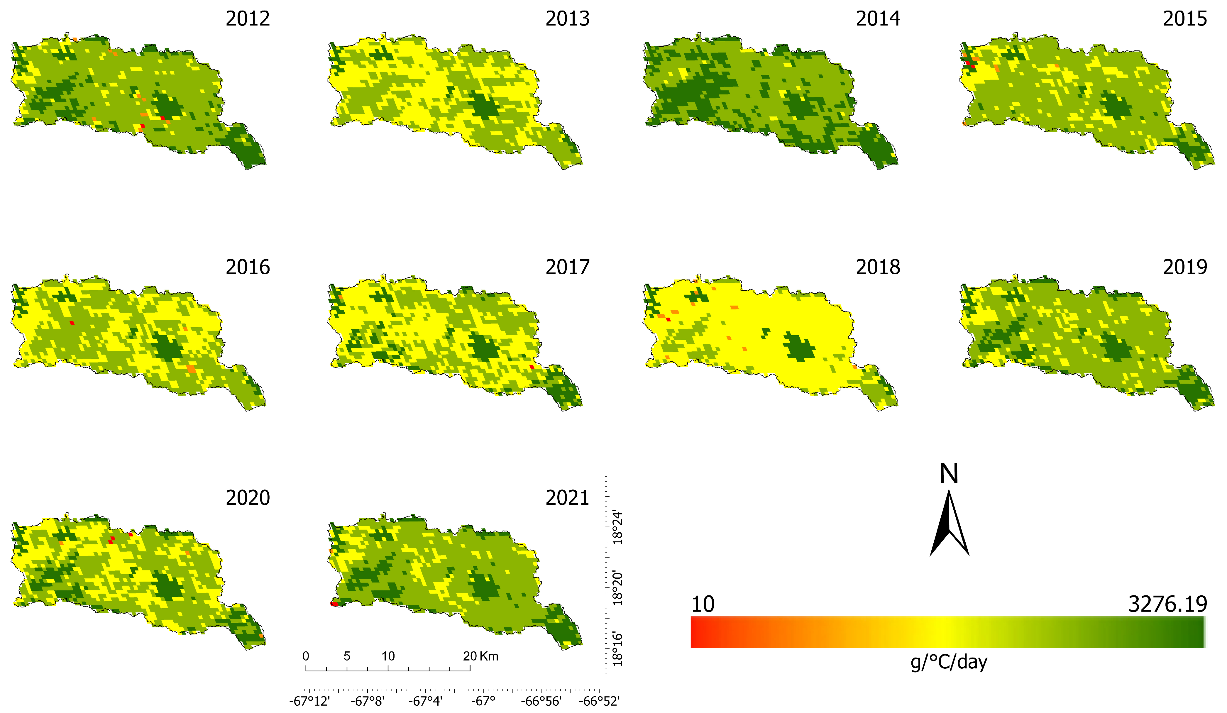
Figure 10 shows the spatial distribution of GPP from 2012 to 2021. Data for 2022 were not available at the time. The GPP varies depending on precipitation, humidity, and vegetation cover, among other factors. After Hurricane Maria in 2017, temperatures and vegetation cover were relatively high and low, respectively. When LST values were high, we obtained higher values of GPP, as GPP and NDVI are more responsive to precipitation.
In 2015, we had an extreme drought period and higher temperatures compared with other years. Therefore, the uptake of CO2 increased, because plant transpiration increases at higher temperatures. Still, a negative correlation between LST and GPP was estimated. In 2018, the lowest GPP values were observed, even though the values of NDVI and GPP seemed to stabilize following the hurricane of 2017. Therefore, although the value of LST is greater, it will not necessarily produce greater values of GPP, as what happened in 2015 when compared with 2016 and 2018. GPP models tend to have large variability and significant trends. Thus, improving observation-based models is needed to accurately estimate carbon uptake [26].
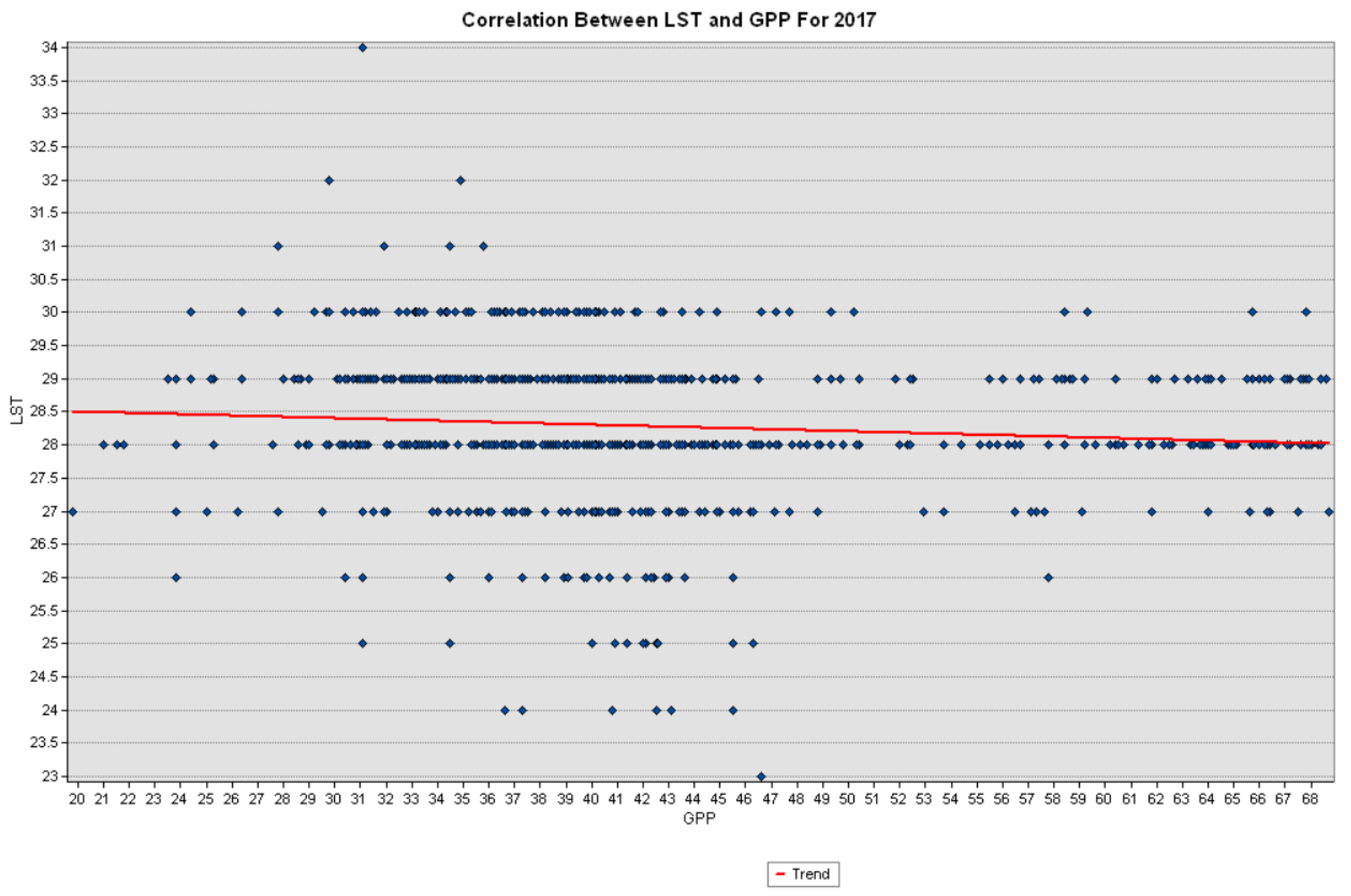
The correlations of GPP with LST and NDVI are shown in Figure 11 and Figure 12, respectively. GPP points with values of 3276.19 g/C/day were not considered, because these values represent nonterrestrial fill values. Therefore, out of the 50 by 50 grid that was made to extract GPP values, around 1000 points were outside the area of study and around 600 points were nonterrestrial fill values.
The correlation tendency between LST and GPP acts like previous LST correlations. As LST increases, GPP decreases, and vice versa. The amount of carbon that plants use during photosynthesis increases when land surface temperature decreases. The effect in our case is more related to available water than it is to surface temperature.
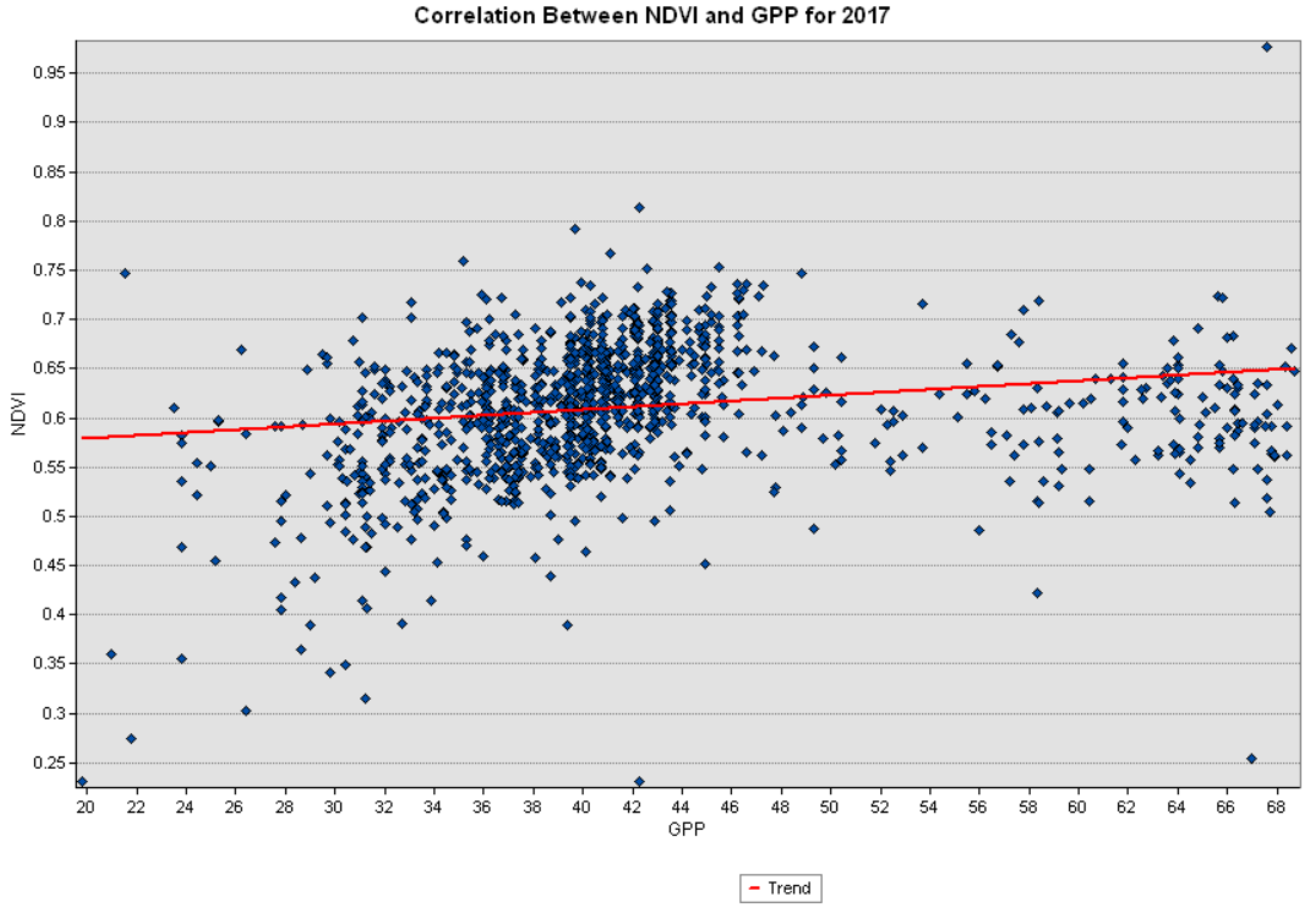
After Hurricane Maria in 2017, most ecosystems were affected and vegetation was reduced considerably compared with other years. The difference in land coverage/greenness, NDVI, can be observed for WRC in 2017 (Figure 3) compared with 2022, after Hurricane Fiona passed over the island. GPP is the amount of carbon that is being exchanged by plants, so it is expected that higher vegetation will produce higher exchange. Thus, correlating NDVI and GPP shows that carbon exchange increases with an increase in NDVI, and vice versa. Nevertheless, values for NDVI and GPP were lower for 2017 compared with other years. The precipitation for 2017 affected the values of NDVI and GPP, as the data were taken after a major atmospheric event.
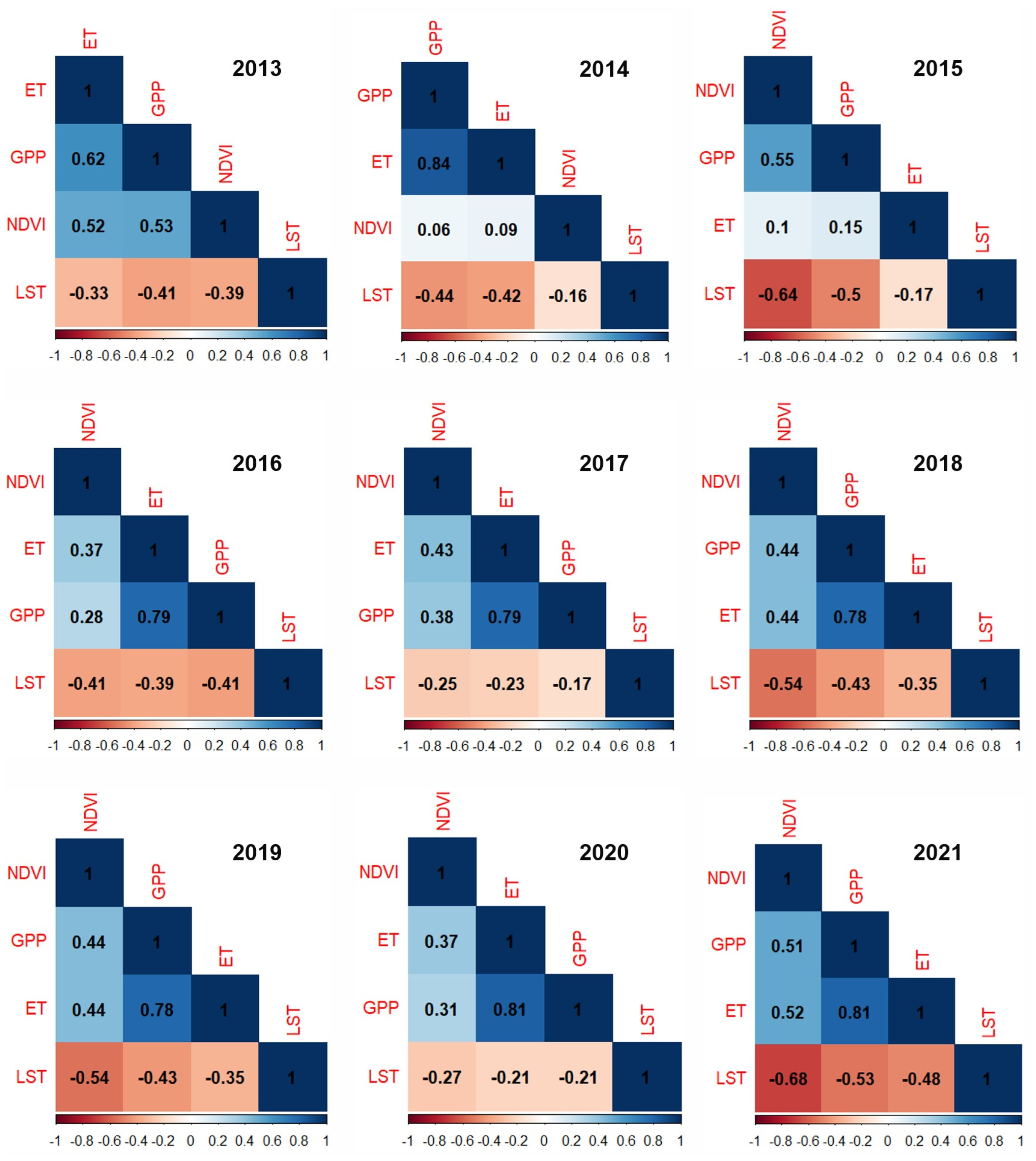
Correlations between the different parameters evaluated for resilience were also investigated using a correlation matrix, as shown in Figure 13. Correlation matrices show the negative and positive correlations between parameters. For the decade evaluated, we saw the same tendency of correlation, where ET positively correlated with NDVI and GPP because these parameters are more responsive to precipitation. On the other hand, LST values negatively correlated with ET, NDVI, and GPP for every year evaluated. In 2013, the matrix value between ET and LST was −0.33, and in 2021, the matrix value was −0.48. In 2015, when the drought period occurred, the correlation values of ET with NDVI and GPP were 0.1 and 0.15, respectively. For 2015, the correlation value between ET and LST was −0.17 (almost no correlation due to the low availability of water). In 2017, the negative correlation values of LST with ET, NDVI, and GPP were −0.23, −0.25, and −0.17, respectively.
4. Discussion
The most common definition of resilience of an ecosystem refers to the capacity of an ecosystem to maintain its functions under the effect of exogenous disturbances [27]. It was expected to observe that urban regions closer to the coast would have less resilience than mountain zones, as mangroves are one of the most threatened ecosystems in the world due to anthropogenic impacts (i.e., urbanization) [28]. An NDVI/GPP positive correlation is usually associated with ecosystem resilience [29,30]. In Figure 3, we can observe the NDVI spatial distribution for 2017 and 2018. Once the ecosystem went through a dramatic change caused by Hurricanes Irma and Maria, it reorganized and reached stability by 2019. Contrarily, the correlation between LST and NDVI cannot be so obviously associated with ecosystem resilience. We can assume that if a yearly correlation was made for 2015, the resilience of the ecosystem would demonstrate signs of being negatively affected. In a study made by Ponce-Campos et al. [31], it was predicted that a prolonged drought in low-productivity grassland would affect the structure of the ecosystem and consequently threaten its resilience. The drought period in 2015, although it may have affected the ecosystem in that period, did not affect the ecosystem’s resilience in the long term. Other authors have also reported that GPP does not always respond the same way to drought under tropical conditions [27] (i.e., some tropical vegetation can tolerate the impacts of reduced precipitation and high temperatures). We can see that throughout the spatial distribution of NDVI in a decade (Figure 3), 2012 and 2022 have similar distributions. Apart from this, there is a positive correlation between NDVI and ET, so the greater the value of NDVI, the greater the value of ET. In Figure 4, we can observe a negative correlation between NDVI and LST. As mentioned by Ghebrezgabher et al. [32], NDVI has a better response to precipitation than it does to temperature, because NDVI is more sensitive to water absorption by plants. At lower temperatures and during moderate or extreme wet events, NDVI will allow us to estimate the resilience of the ecosystem, rather than in conditions with higher and drier temperatures [33]. In general, it was seen from the correlation matrix (Figure 13) that NDVI, ET, and GPP were more responsive to events of high precipitation than to high temperatures/drought periods in the WRC.
The LST values were significantly different in 2015 and 2017 as compared with other years due to extreme climate events (prolonged drought and Hurricanes Irma and Maria, respectively). LST correlations showed that higher temperatures had a negative effect on every other variable evaluated. Tang et al. [34] conducted a study of multiple models for sensing carbon exchange. One of the models presented found that when LST was greater than 273 K, GPP was greatly relative to LST. On the other hand, when LST was less than 273 K, GPP became insensitive. Most of our values of LST are between 27 and 30 Celsius (above 300 K). This means that plant production/GPP was highly influenced by temperature and water availability in the study area. We can also see the effect of LST on ET. In 2015, the average ET was higher than in any of the other years presented in the maps (Figure 7). This is because evaporation at higher temperatures happens at a greater rate if there is a considerable amount of water. Transpiration increases because, at higher temperatures, plants will open their stomata to release water vapor. On the other hand, under extreme drought, evapotranspiration may decrease due to a lack of water. Consequently, plants enter a resting state to preserve water for survival. In 2017, ET rates were lower because of a reduction in land vegetation cover. Overall LST values were negatively correlated with other variables due to the amount of precipitation received for the period evaluated.
ET estimations are important to observe plants’ response to the climate change of the last decade. Climate change is manifesting as prolonged drought periods and more frequent and intense erosive precipitation events [35]. ET estimation can help determine the magnitude of a drought, as low ET is expected under drought conditions [36]. Higher temperatures usually indicate higher rates of ET because of plant stomata, and in extreme scenarios, a decrease in ET because of a lack of water. In this case, ET happened at a higher rate, which promoted an increase in GPP. Again, LST was not the main contributing factor to the ET increase in 2015. This can be observed in Figure 9, where actual ET and GPP are positively correlated. Rosenzweig [37] reported on the relationship between actual ET and productivity, where actual ET is a significant indicator of productivity in mature terrestrial plant communities. This relationship happens because actual ET measures the most important part of plant productivity/GPP: water and solar energy used for photosynthesis. We must acknowledge that even though ET was at its highest in 2015, the GPP rates were not. It has been reported that stressed soil moisture levels are the most crucial driving parameter regarding the productivity of an ecosystem [38]. Due to a lack of precipitation in 2015, soil moisture was low and consequently impacted GPP.
In regards to the spatial distribution of canopy (tree branches and leaves), imperviousness (nonpenetrable surfaces) (Figure 2), and the datasets created for NDVI, GPP, ET, and LST, the areas most affected were either low-canopy areas or areas with a higher concentration of anthropogenic activity. As hypothesized, areas closer to mountains or further away from the coast showed higher resilience. In contrast, plains closer to the coast presented lower resilience. Vegetation was reduced on a greater scale after Hurricanes Irma and Maria. Due to the type of vegetation in urban areas and its density in coastal urban areas, the impact of an atmospheric event such as a hurricane can cause more deterioration to the ecosystem than what is observed closer to mountain ranges. Consequently, the ecosystem takes longer to recover. Long-term degradation of the ecosystem can be mitigated by using native vegetation and maintaining the mangrove areas in the area of study. Alberti and Marzluff [39] proposed that resilience in urban areas is a product of human patterns and is controlled by socioeconomic and biophysical processes. This also means that urban areas are vulnerable to changes in structure due to changes to the natural ecosystem such as land cover, rate of water infiltration, hard covers, and other parameters that are an effect of human activity.
5. Conclusions
Estimation of the resilience of the ecosystem after a significant atmospheric event helps us better understand other changes in the ecosystem. It was expected that atmospheric events would have a lesser impact on ecosystems in areas that are less prone to human activity. In this study, the resilience of the ecosystem had a negative impact in human-active areas and, in contrast, a lesser impact in areas with little or null anthropogenic activity. Segregation of the different land usages will better represent these areas. Nevertheless, NDVI was used as a measure of greenness (representation of plant population). The results observed by the estimations of ET, NDVI, and GPP showed that affected coastal urban areas, after Hurricanes Irma and Maria, took longer to recover and stabilize than less altered areas. This is normal, as humans alter indigenous vegetated areas and substitute them with roads and plants that present reduced ecological resilience in this type of environment.
One of the main limitations of this work was that MOD16A2, used for ET estimation, had many null data values that were amended using the GOES-PRWEB datasets. Daily gap-filled ET products were not available for Puerto Rico. When comparing the data from GOES-PR and MODIS, GOES-PRWEB underestimated actual ET values. Therefore, values of ET estimated from GOES-PRWEB are not to be used for correlation matrices.
In conclusion, we observed that MODIS products can be used for national/large-scale regions rather than small, insular territories where cloud presence can cause under- or overestimation of parameters due to the geographical location of the study area. Additionally, multiday products derived from Landsat can help mitigate the noise caused by cloud coverage.
Author Contributions
Conceptualization, S.F.A.-G.; methodology, Y.N.B.-R. and S.F.A.-G.; formal analysis, Y.N.B.-R. and S.F.A.-G.; investigation, Y.N.B.-R.; resources, S.F.A.-G.; data curation, Y.N.B.-R. and S.F.A.-G.; writing—original draft preparation, Y.N.B.-R.; writing—review and editing, Y.N.B.-R. and S.F.A.-G.; supervision, S.F.A.-G.; project administration, S.F.A.-G.; funding acquisition, S.F.A.-G. All authors have read and agreed to the published version of the manuscript.
Funding
This research was supported by the Agriculture and Food Sciences Facilities and Equipment (AGFEI) program, grant number 2022-70008-38366, from the USDA-National Institute of Food and Agriculture (NIFA). The authors also acknowledge partial support from the College of Agricultural Sciences of the UPRM, a graduate assistantship for Y.N.B.-R., and new faculty seed funds for S.F.A.-G.
Data Availability Statement
The data presented in this study is available upon request to the corresponding author.
Acknowledgments
The authors would like to acknowledge Eric Harmsen, who kindly provided us with raw data from PRWEB servers.
Conflicts of Interest
The authors declare no conflicts of interest.
References
- Chen, Z.; Yin, Q.; Li, L.; Hua, X. Ecosystem health assessment by using remote sensing derived data: A case study of terrestrial region along the coast in Zhejiang Province. In Proceedings of the 2010 IEEE International Geoscience and Remote Sensing Symposium, Honolulu, HI, USA, 25–30 July 2010. [Google Scholar] [CrossRef]
- Pradhan, B.; Yoon, S.; Lee, S. Examining the Dynamics of Vegetation in South Korea: An Integrated Analysis Using Remote Sensing and In Situ Data. Remote Sens. 2024, 16, 300. [Google Scholar] [CrossRef]
- Zektser, I.S.; Loaiciga, H.A. Groundwater fluxes in the global hydrologic cycle: Past, present and future. J. Hydrol. 1993, 144, 405–427. [Google Scholar] [CrossRef]
- Aili, A.; Xu, H.; Waheed, A.; Lin, T.; Zhao, W.; Zhao, X. Drought Resistance of Desert Riparian Forests: Vegetation Growth Index and Leaf Physiological Index Approach. Sustainability 2024, 16, 532. [Google Scholar] [CrossRef]
- Tao, Y.; Meng, E.; Huang, Q. Spatiotemporal Changes and Hazard Assessment of Hydrological Drought in China Using Big Data. Water 2024, 16, 106. [Google Scholar] [CrossRef]
- Latrech, B.; Hermassi, T.; Yacoubi, S.; Slatni, A.; Jarray, F.; Pouget, L.; Ben Abdallah, M.A. Comparative Analysis of Climate Change Impacts on Climatic Variables and Reference Evapotranspiration in Tunisian Semi-Arid Region. Agriculture 2024, 14, 160. [Google Scholar] [CrossRef]
- Wang, Z.; Cui, Z.; He, T.; Tang, Q.; Xiao, P.; Zhang, P.; Wang, L. Attributing the Evapotranspiration Trend in the Upper and Middle Reaches of Yellow River Basin Using Global Evapotranspiration Products. Remote Sens. 2022, 14, 175. [Google Scholar] [CrossRef]
- Wijeratne, V.P.I.S.; Li, G.; Mehmood, M.S.; Abbas, A. Assessing the Impact of Long-Term ENSO, SST, and IOD Dynamics on Extreme Hydrological Events (EHEs) in the Kelani River Basin (KRB), Sri Lanka. Atmosphere 2023, 14, 79. [Google Scholar] [CrossRef]
- Zhang, F.; Tang, P.; Zhou, T.; Liu, J.; Li, F.; Shan, B. Cloud-Based Framework for Precision Agriculture: Optimizing Scarce Water Resources in Arid Environments amid Uncertainties. Agronomy 2024, 14, 45. [Google Scholar] [CrossRef]
- Liu, S.M.; Xu, Z.W.; Zhu, Z.L.; Jia, Z.Z.; Zhu, M.J. Measurements of evapotranspiration from eddy-covariance systems and large aperture scintillometers in the Hai River Basin, China. J. Hydrol. 2013, 487, 24–38. [Google Scholar] [CrossRef]
- Vinukollu, R.K.; Wood, E.F.; Ferguson, C.R.; Fisher, J.B. Global estimates of evapotranspiration for climate studies usingultisensoryr remote sensing data: Evaluation of three process-based approaches. Remote Sens. Environ. 2011, 115, 801–823. [Google Scholar] [CrossRef]
- Tian, F.; Qiu, G.; Yang, Y.; Lü, Y.; Xiong, Y. Estimation of evapotranspiration and its partition based on an extended threetemperature model and MODIS products. J. Hydrol. 2013, 498, 210–220. [Google Scholar] [CrossRef]
- Jung, M.; Reichstein, M.; Ciais, P.; Seneviratne, S.I.; Sheffield, J.; Goulden, M.L.; Bonan, G.; Cescatti, A.; Chen, J.; de Jeu, R.; et al. Recent decline in the global land evapotranspiration trend due to limited moisture supply. Nature 2010, 467, 951–954. [Google Scholar] [CrossRef]
- Mu, Q.; Zhao, M.; Running, S.W. Improvements to a MODIS global terrestrial evapotranspiration algorithm. Remote Sens. Environ. 2011, 115, 1781–1800. [Google Scholar] [CrossRef]
- Harmsen, E.W.; Mecikalski, J.R.; Reventos, V.J.; Álvarez-Pérez, E.; Uwakweh, S.S.; Adorno-García, C. Water and energy balance model GOES-PRWEB: Development and validation. Hydrology 2021, 8, 113. [Google Scholar] [CrossRef]
- de Oliveira, M.L.; Dos Santos, C.A.C.; de Oliveira, G.; Silva, M.T.; da Silva, B.B.; Cunha, J.E.B.L.; Ruhoff, A.; Santos, C.A.G. Remote sensing-based assessment of land degradation and drought impacts over terrestrial ecosystems in Northeastern Brazil. Sci. Total Environ. 2022, 20, 155490. [Google Scholar] [CrossRef]
- Beck, H.E.; Zimmermann, N.E.; McVicar, T.R.; Vergopolan, N.; Berg, A.; Wood, E.F. Present and future Köppen-Geiger climate classification maps at 1-km resolution. Sci. Data 2018, 5, 180214. [Google Scholar] [CrossRef] [PubMed]
- Lugo, J.; Diaz, D. Developing Sustinable Planing for Heritage Conservation in the Tropics: A GIS-Based Risk and Vulnerability Assessment Profile for Historic Archives in Puerto Rico. WIT Trans. Ecol. Environ. 2018, 217, 613–623. [Google Scholar] [CrossRef]
- Kenner, B.; Russell, D.; Valdes, C.; Sowell, A.; Pham, X.; Terán, A.; Kaufman, J. Puerto Rico’s Agricultural Economy in the Aftermath of Hurricanes Irma and Maria: A Brief Overview. U.S. Department of Agriculture, Economic Research Service, AP-114. April 2023. Available online: https://www.ers.usda.gov/webdocs/publications/106261/ap-114.pdf?v=3172 (accessed on 22 December 2023).
- Running, S.; Mu, Q.; Zhao, M. MODIS/Terra Net Evapotranspiration 8-Day L4 Global 500m SIN Grid V061 [Data Set]; NASA EOSDIS Land Processes Distributed Active Archive Center: Sioux Falls, SD, USA, 2021. [Google Scholar] [CrossRef]
- Reddy, S.N.; Manikiam, B. Land Surface Temperature Retrieval from LANDSAT data using Emissivity Estimation. Int. J. Appl. Eng. Res. 2017, 12, 9679–9687. [Google Scholar]
- Vanhellemont, Q. Combined land surface emissivity and temperature estimation from Lansat 8 OLI and TIRS. ISPRS J. Photogramm. Remote Sens. 2020, 166, 390–402. [Google Scholar] [CrossRef]
- Didan, K. MODIS/Terra Vegetation Indices 16-Day L3 Global 250m SIN Grid V061 [Data Set]; NASA EOSDIS Land Processes Distributed Active Archive Center: Sioux Falls, SD, USA, 2021. [Google Scholar] [CrossRef]
- Running, S.; Mu, Q.; Zhao, M. MODIS/Terra Gross Primary Productivity 8-Day L4 Global 500m SIN Grid V061 [Data Set]; NASA EOSDIS Land Processes Distributed Active Archive Center: Sioux Falls, SD, USA, 2021. [Google Scholar] [CrossRef]
- Villalobos, F.J.; Testi, L.; Mateos, L.; Fereres, E. Soil Temperature and Soil Heat Flux. In Principles of Agronomy for Sustainable Agriculture, 1st ed.; Springer: Berlin/Heidelberg, Germany, 2017; pp. 69–77. [Google Scholar] [CrossRef]
- Anav, A.; Friedlingstein, P.; Beer, C.; Ciais, P.; Harper, A.; Jones, C.; Murray-Tortarolo, G.; Papale, D.; Parazoo, N.C.; Peylin, P.; et al. Spatiotemporal patterns of terrestrial gross primary production: A review. Rev. Geophys. 2015, 53, 785–818. [Google Scholar] [CrossRef]
- Seixas, H.T.; Brunsell, N.A.; Moraes, E.C.; Oliveira, G.; Mataveli, G. Exploring the ecosystem resilience concept with land surface model scenarios. Ecol. Modell. 2022, 464, 109817. [Google Scholar] [CrossRef]
- Fickert, T. To Plant or Not to Plant, That Is the Question: Reforestation vs. Natural Regeneration of Hurricane-Disturbed Mangrove Forests in Guanaja (Honduras). Forests 2020, 11, 1068. [Google Scholar] [CrossRef]
- Bryant, T.; Waring, K.; Sánchez Meador, A.; Bradford, J.B. A framework for quantifying resilience to forest disturbance. Front. For. Glob. Chang. 2019, 2, 56. [Google Scholar] [CrossRef]
- Zampieri, M.; Grizzetti, B.; Toreti, A.; Palma, P.; Collati, A. Rise and fall of vegetation annual primary production resilience to climate variability projected by a large ensemble of Earth System Models’ simulations. Environ. Res. Lett. 2021, 16, 105001. [Google Scholar] [CrossRef]
- Ponce-Campos, G.E.; Moran, M.S.; Huete, A.; Zhang, Y.; Bresloff, C.; Huxman, T.E.; Eamus, D.; Bosch, D.D.; Buda, A.R.; Gunter, S.A.; et al. Ecosystem resilience despite large-scale altered hydroclimatic conditions. Nature 2013, 494, 349–352. [Google Scholar] [CrossRef] [PubMed]
- Ghebrezgabher, M.G.; Yang, T.; Yang, X.; Sereke, T.E. Assessment of NDVI variations in responses to climate change in the Horn of Africa. Egypt. J. Remote Sens. Space Sci. 2020, 23, 249–261. [Google Scholar] [CrossRef]
- Hossain, L.; Li, J. NDVI-based vegetation dynamics and its resistance and resilience to different intensities of climatic events. Glob. Ecol. Conserv. 2021, 30, e01768. [Google Scholar] [CrossRef]
- Tang, X.; Li, H.; Desai, A.R.; Xu, X.; Xie, J. Comparison of multiple models for remote sensing of carbon exchange using MODIS data in conifer-dominated forests. Int. J. Remote Sens. 2014, 35, 8252–8271. [Google Scholar] [CrossRef]
- Panagos, P.; Borelli, P.; Matthews, F.; Liakos, L.; Bezak, N.; Diodato, N.; Ballabio, C. Global rainfall erosivity projections for 2050 and 2070. J. Hydrol. 2022, 610, 127865. [Google Scholar] [CrossRef]
- Zhan, X.; Fang, L.; Yin, J.; Schull, M.; Liu, J.; Hain, C.; Anderson, M.; Kustas, W.; Kalluri, S. Remote Sensing of Evapotranspiration for Global Drought Monitoring. In Global Drought and Flood: Observation, Modeling, and Prediction, 1st ed.; Geophysical Monograph Series; John Wiley & Sons: Hoboken, NJ, USA, 2021. [Google Scholar] [CrossRef]
- Rosenzweig, M.L. Net Primary Productivity of Terrestrial Communities: Prediction from Climatological Data. Am. Nat. 1968, 102, 67–74. [Google Scholar] [CrossRef]
- Falloon, P.; Jones, C.D.; Ades, M.; Paul, K. Direct soil moisture controls of future global soil carbon changes: An important source of uncertainty. Glob. Biogeochem. Cycles 2011, 25, 3. [Google Scholar] [CrossRef]
- Alberti, M.; Marzluff, J.M. Ecological resilience in urban ecosystems: Linking urban patterns to human and ecological functions. Urban Ecosyst. 2004, 7, 241–265. [Google Scholar] [CrossRef]
Figure 1.
Land use/land cover map of Puerto Rico. The Culebrinas River Watershed (CRW) is located in the northwest region of Puerto Rico. It includes several municipalities and offers diverse ecosystem services.
Figure 1.
Land use/land cover map of Puerto Rico. The Culebrinas River Watershed (CRW) is located in the northwest region of Puerto Rico. It includes several municipalities and offers diverse ecosystem services.

Figure 2.
Spatial distribution of imperviousness within the Culebrinas River Watershed in Western Puerto Rico. The urban areas can be identified in red clusters as part of the main towns of the municipalities of Aguadilla, Aguada, Moca, and San Sebastian.
Figure 2.
Spatial distribution of imperviousness within the Culebrinas River Watershed in Western Puerto Rico. The urban areas can be identified in red clusters as part of the main towns of the municipalities of Aguadilla, Aguada, Moca, and San Sebastian.

Figure 3.
Spatial distribution of NDVI estimated from MOD13Q1 between 2012 and 2022. Data for MOD17A2 (GPP) were not available for 2012 and 2022.
Figure 3.
Spatial distribution of NDVI estimated from MOD13Q1 between 2012 and 2022. Data for MOD17A2 (GPP) were not available for 2012 and 2022.

Figure 4.
Correlation between land surface temperature and the normalized difference vegetation index.
Figure 4.
Correlation between land surface temperature and the normalized difference vegetation index.

Figure 5.
Spatial distribution for estimated from Landsat 8–9 OLI-TIRS between 2013 and 2022.

Figure 6.
Correlation between land surface temperature and actual evapotranspiration for 2015.

Figure 7.
Spatial distribution of ET estimated from MOD16A2 between 2012 and 2022.

Figure 8.
Correlation between normalized difference vegetation index and actual ET for 2017.

Figure 9.
Correlation between gross primary production and evapotranspiration for 2015.

Figure 10.
Spatial distribution of GPP estimated from MOD17A1; an 8-day composite with a 500 m resolution.
Figure 10.
Spatial distribution of GPP estimated from MOD17A1; an 8-day composite with a 500 m resolution.

Figure 11.
Correlation between land surface temperature and gross primary production for 2017.

Figure 12.
Correlation between normalized difference vegetation index and gross primary production for 2017.
Figure 12.
Correlation between normalized difference vegetation index and gross primary production for 2017.

Figure 13.
Correlation between NDVI, LST, ET, and GPP from 2013 to 2021.


Table 1.
Metadata of the satellite images from 2013–2022 for Landsat 8–9 OLI-TRIS.
| Variables | Description | Values |
|---|---|---|
| K1 | Thermal constants Band 10 | 774.8853 |
| K2 | 1321.0789 | |
| ML | Band-specific multiplicative rescaling factor | 3.34 × 10⁻⁴ |
| AL | Band-specific additive rescaling factor | 0.1 |
| Lmax | Maximum value or radiance, Band 10 | 22.0018 |
| Lmin | Minimum value or radiance, Band 10 | 0.10033 |
| Qcalmax | Maximum values of quantized calibration, Band 10 | 65,535 |
| Qcalmin | Minimum value of quantized calibration, Band 10 | 1 |
Table 2.
Estimated range of NDVI, LST, ET, and GPP for WRC from 2012 to 2022. High values of GPP, 3.2762 kg, correspond to land cover assigned as urban.
Table 2.
Estimated range of NDVI, LST, ET, and GPP for WRC from 2012 to 2022. High values of GPP, 3.2762 kg, correspond to land cover assigned as urban.
| Year | NDVI | LST | ET | GPP | ||||
|---|---|---|---|---|---|---|---|---|
| UNITS | ||||||||
| - | °C | mm/day | kg/°C/day | |||||
| Low | High | Low | High | Low | High | Low | High | |
| 2012 | 0.0981 | 0.986 | - | - | 1.8374 | 7.8125 | 0.0116 | 3.2762 |
| 2013 | 0.2229 | 0.9195 | 19.1045 | 33.2603 | 1.2250 | 7.1500 | 0.0235 | 3.2762 |
| 2014 | 0.265 | 0.9176 | 22 | 34 | 2.2000 | 7.3375 | 0.0372 | 3.2762 |
| 2015 | 0.2403 | 0.9373 | 22.6019 | 39.3491 | 1.5625 | 8.0375 | 0.0115 | 3.2762 |
| 2016 | 0.1296 | 0.9941 | 20.6582 | 34.6485 | 1.9875 | 6.8375 | 0.0145 | 3.2762 |
| 2017 | 0.0774 | 0.9768 | 22 | 35.4926 | 1.9375 | 5.8375 | 0.0147 | 3.2762 |
| 2018 | 0.4147 | 0.9119 | 23.3586 | 35.6335 | 1.3750 | 4.6125 | 0.0128 | 3.2762 |
| 2019 | 0.3045 | 0.9622 | 23 | 34 | 1.3999 | 6.1750 | 0.0241 | 3.2762 |
| 2020 | 0.2037 | 0.9885 | 21.1934 | 35 | 1.8125 | 5.5008 | 0.0089 | 3.2762 |
| 2021 | 0.2328 | 0.9346 | 22.9827 | 34.1233 | 1.5000 | 8.4250 | 0.0121 | 3.2762 |
| 2022 | 0.2909 | 0.9323 | 22.8446 | 35.9824 | 2.2000 | 8.3125 | - | - |
Disclaimer/Publisher’s Note: The statements, opinions and data contained in all publications are solely those of the individual author(s) and contributor(s) and not of MDPI and/or the editor(s). MDPI and/or the editor(s) disclaim responsibility for any injury to people or property resulting from any ideas, methods, instructions or products referred to in the content. |
© 2024 by the authors. Licensee MDPI, Basel, Switzerland. This article is an open access article distributed under the terms and conditions of the Creative Commons Attribution (CC BY) license (https://creativecommons.org/licenses/by/4.0/).
Share and Cite
MDPI and ACS Style
Bonilla-Roman, Y.N.; Acuña-Guzman, S.F. Resilience of an Urban Coastal Ecosystem in the Caribbean: A Remote Sensing Approach in Western Puerto Rico. Earth 2024, 5, 72-89. https://doi.org/10.3390/earth5010004
AMA Style
Bonilla-Roman YN, Acuña-Guzman SF. Resilience of an Urban Coastal Ecosystem in the Caribbean: A Remote Sensing Approach in Western Puerto Rico. Earth. 2024; 5(1):72-89. https://doi.org/10.3390/earth5010004
Chicago/Turabian StyleBonilla-Roman, Yadiel Noel, and Salvador Francisco Acuña-Guzman. 2024. "Resilience of an Urban Coastal Ecosystem in the Caribbean: A Remote Sensing Approach in Western Puerto Rico" Earth 5, no. 1: 72-89. https://doi.org/10.3390/earth5010004