Entropy Estimators for Markovian Sequences: A Comparative Analysis

Abstract

Entropy estimation is a fundamental problem in information theory that has applications in various fields, including physics, biology, and computer science. Estimating the entropy of discrete sequences can be challenging due to limited data and the lack of unbiased estimators. Most existing entropy estimators are designed for sequences of independent events and their performances vary depending on the system being studied and the available data size. In this work, we compare different entropy estimators and their performance when applied to Markovian sequences. Specifically, we analyze both binary Markovian sequences and Markovian systems in the undersampled regime. We calculate the bias, standard deviation, and mean squared error for some of the most widely employed estimators. We discuss the limitations of entropy estimation as a function of the transition probabilities of the Markov processes and the sample size. Overall, this paper provides a comprehensive comparison of entropy estimators and their performance in estimating entropy for systems with memory, which can be useful for researchers and practitioners in various fields.

1. Introduction

The entropy associated with a random variable is a measure of its uncertainty or diversity, taking large values for a highly unpredictable random variable (i.e., all outcomes equally probable) and low values for a highly predictable one (i.e., one or few outcomes much more probable than the others). As such, the concept has found multiple applications in a variety of fields including but not limited to nonlinear dynamics, statistical physics, information theory, biology, neuroscience, cryptography, and linguistics [1,2,3,4,5,6,7,8,9,10,11,12,13].

Due to its mathematical simplicity and clear interpretation, Shannon’s definition is the most widely used measure of entropy [14]. For a discrete random variable X with L distinct possible outcomes $x_1,\dots ,x_L$, the Shannon entropy reads

$$H\left[X\right]=-\sum _{i=1}^{L}p\left(x_i\right)ln\left(p\left(x_i\right)\right),$$

(1)

where $p\left(x_i\right)$ denotes the probability that the random variable X takes the value $x_i$.

It often occurs in practice that the probability distribution of the variable X is unknown, either due to mathematical difficulties or to the lack of deep knowledge of the details of the underlying experiment described by the random variable X. In those situations, it is not possible to compute the entropy using Equation (1) directly. In general, our information is restricted to a finite set of ordered data resulting from the observation of the outcomes obtained by repeating a large number of times, N, the experiment. Hence, the goal is to estimate H from the ordered sequence $S=X_1,\dots ,X_N$, where each $X_j\in {\left\{x_i\right\}}_{i=1}^L$ with $j=1,\dots ,N$.

A numerical procedure that provides an approximation to the true value of H based on the sequence S is called an entropy estimator. As the sequence S is random, it is clear that an entropy estimator is itself a random variable, taking different values for different realizations of the sequence of N outcomes. It would be highly desirable to have an unbiased entropy estimator, i.e., an estimator whose average value coincides with the true result H for all values of the sequence length N. However, it can be proven that such an estimator does not exist [15] and that, apart from the unavoidable statistical errors due to the finite number N of data of the sample (and which typically scale as $N^{-1/2}$), all estimators present systematic errors which are in general difficult to evaluate properly. Therefore, a large effort has been devoted to the development of entropy estimators that, although necessarily biased, provide a good value for H with small statistical and systematic errors [16].

The problem of finding a good estimator with small errors becomes more serious when the number of data N is relatively small. Indeed, when the sizes of available data are much larger than the possible outcomes ($N\gg L$), it is not difficult to estimate H accurately, and all of the most popular estimators are naturally satisfactory in this regime. The task becomes much harder as the numbers L and N come closer to each other. It is particularly difficult in the undersampled regime ($N\lesssim L$) [17], where some, or potentially many, possible outcomes may not be observed in the sequence. It is in this regime where the difference in accuracy among the available estimators is more significant.

We emphasize that the discussed difficulties already appear for independent identically distributed (i.i.d.) random variables. Precisely, the previous literature has largely dealt with entropy estimators proposed for sequences of i.i.d. random variables [16,18,19,20,21]. However, it is not clear that real data arising from experimental observation can be described with i.i.d. random variables due to the ubiquitous presence of data correlations. The minimal correlations in discrete sequences are of a Markovian nature. Then, how do the main entropy estimators behave for Markovian sequences?

The purpose of this work is to make a detailed comparison of some of the most widely used entropy estimators in systems whose future is conditionally independent of the past (Markovian). In Markovian sequences, correlations stem from the fundamental principle that the probability of a data value appearing at a specific time depends on the value observed in the preceding time step. Markov chains have been used to model systems in a large variety of fields such as statistical physics [22], molecular biology [23], weather forecast [24], and linguistics [25], just to mention a few. Below, we analyze the strengths and weaknesses of estimators tested in a correlated series of numerically generated data. We compare the performances for the estimators that have shown to give good results for independent sequences [16]. For definiteness, we below consider Markovian sequences of binary data. Furthermore, the calculation of relevant quantities in information theory, such as entropy rate and predictability gain [26], requires estimating the block entropy of a sequence, obtained from the estimation of the entropy associated not to a single result, but to a block of consecutive results. As we will argue in the following sections, the construction of overlapping blocks induces correlations amongst them, even if the original sequence is not correlated. The calculation of the block entropy is also a tool that can be used to estimate the memory of a given sequence [27], which is of utmost importance when dealing with strongly correlated systems [28,29,30,31,32,33].

The rest of the paper is organized as follows. In Section 2, we make a brief overview of the ten entropy estimators being considered in this study, nine of which are already known in the literature and an additional estimator built from results presented in ref. [34], which is further developed in this work. In Section 3, we present the results of our comparative analysis of these estimators in two Markovian cases: (A) binary sequences; and (B) in an undersampled regime. Section 4 contains the conclusions and an outlook. Finally, in Appendix A we provide a new interpretation in terms of geometric distributions of an estimator which is widely used as the starting point to construct others, and in Appendix B we prove the equivalence between a dynamics of block sequences and a Markovian random variable.

2. Materials and Methods

In the following, we will use the notation $\widehat{a}$ to refer to a numerical estimator of the quantity a. The bias of $\widehat{a}$ is defined as

$$B\left[\widehat{a}\right]=〈\widehat{a}〉-a,$$

(2)

where $〈\widehat{a}〉$ represents the expected value of $\widehat{a}$. The estimator $\widehat{a}$ is said to be unbiased if $B\left[\widehat{a}\right]=0$. The dispersion of $\widehat{a}$ is given by the standard deviation

$$\sigma \left[\widehat{a}\right]=\sqrt{\langle {\widehat{a}}^2\rangle -{\langle \widehat{a}\rangle }^2}.$$

(3)

Ideally, $\widehat{a}$ should be as close to the true value a as possible. Therefore, it is desirable that $\widehat{a}$ has both low bias and low standard deviation. With this in mind, it is natural to consider the mean squared error of an estimator, given by

$$\mathrm{MSE}\left[\widehat{a}\right]=B{\left[\widehat{a}\right]}^2+\sigma {\left[\widehat{a}\right]}^2,$$

(4)

to assess its quality. Hence, when comparing estimators of the same variable, the one with the lowest mean squared error is preferable.

Given an estimator $\widehat{H}$ of the entropy, its k-th moment can be computed as

$$\begin{array}{c}\hfill \langle {\widehat{H}}^k\rangle =\sum _{S}P\left(S\right)\widehat{H}{\left(S\right)}^k,\end{array}$$

(5)

where the sum runs over all possible sequences $S=X_1,\dots ,X_N$ of length N and $\widehat{H}\left(S\right)$ is the value that the estimator takes on in this sequence. The probability $P\left(S\right)$ of observing the sequence S depends on whether S is correlated or not. For example, if S is an independent sequence, $P\left(S\right)$ can be calculated as

$$P\left(S\right)=\prod _{i=1}^{N}p\left(X_i\right).$$

(6)

For correlated sequences, Equation (6) no longer holds. Consider a Markovian system, in which the probability of the next event only depends on the current state. In other words, the transition probabilities satisfy

$$\begin{array}{c}\hfill P(X_s=x_j|X_{s-1}=x_{\ell },\dots ,X_1=x_k)=P(X_s=x_j|X_{s-1}=x_{\ell }),\end{array}$$

(7)

with s the position in the series. A homogeneous Markov chain is one in which the transition probabilities are independent of the time step s. Therefore, a homogeneous Markov chain is completely specified given the $L\times L$ matrix of transition probabilities $p\left(x_j\right|x_{\ell })=P(X_s=x_j|X_{s-1}=x_{\ell }),j,\ell =1,\dots ,L$. In this case, the probability of observing the sequence S can be calculated as

$$P\left(S\right)=p\left(X_1\right)\prod _{i=1}^{N-1}p\left(X_{i+1}\right|X_i).$$

(8)

where we have applied Equation (7) successively.

The calculation of $P\left(S\right)$ can be generalized to an m-order Markov chain defined by the transition probabilities:

$$\begin{array}{c}\hfill P(X_s=x_j|X_{s-1}=x_{\ell },\dots ,X_1=x_k)=P(X_s=x_j|X_{s-1}=x_{\ell },\dots ,X_{s-m}=x_u),\end{array}$$

(9)

that depend on the m previous results of the random variable.

It is clear that the moments of the estimator $\widehat{H}$, and consequently its performance given by its mean squared error, depend on the correlations of the system being analyzed.

Most of the entropy estimators considered in this work only depend on the number of times each outcome occurs in the sequence. In this case, the calculation of the moments of the estimator can be simplified for independent and Markovian systems considering the corresponding multinomial distributions [35].

Several entropy estimators were developed with the explicit assumption that the sequences being analyzed are uncorrelated [36,37]. The main assumption is that the probability of the number of times $n_i$ that the outcome $x_i$ occurs in a sequence of length N follows a binomial distribution,

$$P\left(n_i\right)=\left(\genfrac{}{}{0pt}{}{N}{n_i}\right)p{\left(x_i\right)}^{n_i}{(1-p\left(x_i\right))}^{N-n_i}.$$

(10)

This approach is not valid when dealing with general Markovian sequences because Equation (10) no longer holds. Instead, the Markovian binomial distribution [38] should be used, or more generally, the Markovian multinomial distribution [35]. Even for entropy estimators that were not developed directly using Equation (10), their performance is usually only analyzed for independent sequences [16]. Hence, the need to compare and evaluate the different estimators in Markov chains.

Even though there exists a plethora of entropy estimators in the literature [15,39,40,41,42,43,44,45,46,47], we here focus on nine of the most commonly employed estimators, and we also propose a new estimator, constructed from known results [34].

2.1. Maximum Likelihood Estimator

The maximum likelihood estimator (MLE) (also known as plug-in estimator) simply consists of replacing the exact probabilities in Equation (1) for the estimated frequencies,

$$\widehat{p}\left(x_i\right)={\displaystyle \frac{{\widehat{n}}_i}{N}},$$

(11)

where ${\widehat{n}}_i$ is the number of times that the outcome $x_i$ is observed in the given sequence. It is well known that Equation (11) is an unbiased estimator of $p\left(x_i\right)$, but the MLE estimator, given by

$${\widehat{H}}^{\mathrm{MLE}}=-\sum _{i=1}^L\widehat{p}\left(x_i\right)ln\left(\widehat{p}\left(x_i\right)\right),$$

(12)

is negatively biased [15], i.e., $\langle {\widehat{H}}^{\mathrm{MLE}}\rangle -H<0$.

2.2. Miller–Madow Estimator

The idea behind the Miller–Madow estimator (MM) [48] is to correct the bias of ${\widehat{H}}^{\mathrm{MLE}}$ up to the first order in $1/N$, resulting in

$${\widehat{H}}^{\mathrm{MM}}={\widehat{H}}^{\mathrm{MLE}}+{\displaystyle \frac{N_0-1}{2N}},$$

(13)

where $N_0$ is the number of different elements present in the sequence. Corrections of higher order are not considered because they include the unknown probabilities $p\left(x_i\right)$ [49].

2.3. Nemenman–Shafee–Bialek Estimator

A large family of entropy estimators are derived by estimating the probabilities using a Bayesian framework [40,44,50,51,52,53]. The Nemenman–Shafee–Bialek estimator (NSB) [54,55,56] provides a novel Bayesian approach that, unlike traditional methods, does not rely on strong prior assumptions on the probability distribution. Instead, this method uses a mixture of Dirichlet priors, designed to produce an approximately uniform distribution of the expected entropy value. This ensures that the entropy estimate is not exceedingly biased by prior assumptions.

The Python implementation developed in ref. [57] was used in this paper for the calculations of the NSB estimator.

2.4. Chao–Shen Estimator

The Chao–Shen estimator (CS) [18] takes into account two corrections to Equation (12) to reduce its bias: first, a Horvitz–Thompson adjustment [58] to account for missing elements in a finite sequence; second, a correction to the estimated probabilities, ${\widehat{p}}^{\mathrm{CS}}\left(x_i\right)={\widehat{C}}^{\mathrm{CS}}\widehat{p}\left(x_i\right)$, leading to

$${\widehat{C}}^{\mathrm{CS}}=1-{\displaystyle \frac{N_1}{N}},$$

(14)

where $N_1$ is the number of elements that appear only once in the sequence.

The Chao–Shen entropy estimator is then

$${\widehat{H}}^{\mathrm{CS}}=-\sum _{x_i\in S}{\displaystyle \frac{{\widehat{p}}^{\mathrm{CS}}\left(x_i\right)ln\left({\widehat{p}}^{\mathrm{CS}}\left(x_i\right)\right)}{1-{(1-{\widehat{p}}^{\mathrm{CS}}\left(x_i\right))}^N}}.$$

(15)

2.5. Grassberger Estimator

Assuming that all $p\left(x_i\right)\ll 1$, the probability distribution of each $n_i$ can be approximated by a Poisson distribution. Following this idea, Grassberger (G) derived the estimator presented in ref. [36] by first considering Rényi entropies of order q [59]:

$$H\left(q\right)={\displaystyle \frac{1}{q-1}}ln\sum _{i=1}^{L}p{\left(x_i\right)}^q.$$

(16)

Taking into account that the Shannon case can be recovered by taking the limit $q\to 1$, the author proposed a low bias estimator for the quantity $p^q$, for an arbitrary q. This approach led to the estimator given by

$${\widehat{H}}^{\mathrm{G}}=ln\left(N\right)-{\displaystyle \frac{1}{N}}\sum _{i=1}^L{\widehat{n}}_i{G}_{{\widehat{n}}_i},$$

(17)

with $G_1=-\gamma -ln2$, $G_2=2-\gamma -ln2$, and the different values of $G_{{\widehat{n}}_i}$ computed using the recurrence relation

$$\begin{array}{cc}\hfill G_{2n+1}& =G_{2n}\hfill \end{array}$$

(18)

$$\begin{array}{cc}\hfill G_{2n+2}& =G_{2n}+{\displaystyle \frac{2}{2n+1}},\hfill \end{array}$$

(19)

where $\gamma =0.57721\dots$ is Euler’s constant.

2.6. Bonachela–Hinrichsen–Muñoz Estimator

The idea behind the Bonachela–Hinrichsen–Muñoz estimator (BHM) [37] is to make use of Equation (10) to find a balanced estimator of the entropy that, on average, minimizes the mean squared error. The resulting estimator is given by

$${\widehat{H}}^{\mathrm{BHM}}={\displaystyle \frac{1}{N+2}}\sum _{i=1}^L({\widehat{n}}_i+1)\sum _{j={\widehat{n}}_i+2}^{N+2}{\displaystyle \frac{1}{j}}.$$

(20)

2.7. Shrinkage Estimator

The estimator proposed by Hausser and Strimmer [20] (HS) is a shrinkage-type estimator [60], in which the probabilities are estimated as an average of two models:

$${\widehat{p}}^{\mathrm{HS}}\left(x_i\right)=\alpha {\displaystyle \frac{1}{L}}+(1-\alpha )\widehat{p}\left(x_i\right),$$

(21)

where the weight $\alpha$ is chosen so that the resulting estimator ${\widehat{p}}^{\mathrm{HS}}$ has lower mean squared error than $\widehat{p}$ and is calculated by [61]

$$\alpha =\min \left(1,{\displaystyle \frac{1-{\sum }_{i=1}^L{\left(\widehat{p}\left(x_i\right)\right)}^2}{(N-1){\sum }_{i=1}^L{(1/L-\widehat{p}\left(x_i\right))}^2}}\right).$$

(22)

Hence, the shrinkage estimator is

$${\widehat{H}}^{\mathrm{HS}}=-\sum _{i=1}^L{\widehat{p}}^{\mathrm{HS}}\left(x_i\right)ln\left({\widehat{p}}^{\mathrm{HS}}\left(x_i\right)\right).$$

(23)

2.8. Chao–Wang–Jost Estimator

The Chao–Wang–Jost estimator (CWJ) [62] uses the series expansion of the logarithm function, as well as a correction to account for the missing elements in the sequence. This estimator is given by

$$\begin{array}{cc}\hfill {\widehat{H}}^{\mathrm{CWJ}}& =\sum _{i=1}^L{\displaystyle \frac{{\widehat{n}}_i}{N}}(\psi \left(N\right)-\psi \left({\widehat{n}}_i\right))+{\displaystyle \frac{N_1}{N}}{(1-A)}^{1-N}\left(-ln\left(A\right)-\sum _{j=1}^{N-1}{\displaystyle \frac{1}{j}}{(1-A)}^j\right),\hfill \end{array}$$

(24)

where $\psi \left(z\right)$ is the digamma function and A is given by

$$\begin{array}{c}\hfill \begin{array}{c}\hfill A=\left\{\begin{array}{cc}{\displaystyle \frac{2N_2}{(N-1)N_1+2N_2}},\hfill & \mathrm{if}{N}_2>0,\hfill \\ {\displaystyle \frac{2}{(N-1)(N_1-1)+2}},\hfill & \mathrm{if}{N}_2=0,N_1>0,\hfill \\ 1,\hfill & \mathrm{if}{N}_1=N_2=0,\hfill \end{array}\right.\end{array}\end{array}$$

(25)

with $N_1$ and $N_2$ the number of elements that appear once and twice, respectively, in the sequence.

In the supplementary material of ref. [62], it is proven that the first sum in Equation (24) is the same as the leading terms of the estimators developed in refs. [41,42]. In Appendix A, we show that each term in this sum is also equivalent to an estimator that takes into account the number of observations made prior to the occurrence of the element $x_i$.

2.9. Correlation Coverage-Adjusted Estimator

The correlation coverage-adjusted estimator (CC) [27] uses the same ideas that support Equation (15) but considers a different correction to the probabilities, ${\widehat{p}}^{\mathrm{CC}}\left(x_i\right)$ =${\widehat{C}}^{\mathrm{CC}}\widehat{p}\left(x_i\right)$, where now ${\widehat{C}}^{\mathrm{CC}}$ is calculated sequentially taking into account previously observed data,

$${\widehat{C}}^{\mathrm{CC}}=1-\sum _{j=1}^{N^{\prime }}{\displaystyle \frac{1}{N^{\prime }+j}}I(X_{N^{\prime }+j}\notin (X_1,\dots ,X_{N^{\prime }+j-1})),$$

(26)

where $N^{\prime }\equiv N/2$ and the function $I\left(Z\right)$ yields 1 if the event Z is true and 0 otherwise. By construction, this probability estimator considers possible correlations in the sequence.

Then, the CC estimator is given by

$${\widehat{H}}^{\mathrm{CC}}=-\sum _{x_i\in S}{\displaystyle \frac{{\widehat{p}}^{\mathrm{CC}}\left(x_i\right)ln\left({\widehat{p}}^{\mathrm{CC}}\left(x_i\right)\right)}{1-{(1-{\widehat{p}}^{\mathrm{CC}}\left(x_i\right))}^N}}.$$

(27)

2.10. Corrected Miller–Madow Estimator

In ref. [34] it is shown that the bias of the MLE estimator can be approximated based on a Taylor expansion as

$$B\left[{\widehat{H}}^{\mathrm{MLE}}\right]\approx -{\displaystyle \frac{N_0-1}{2N}}-{\displaystyle \frac{1}{N}}\sum _{l=1}^{\infty }K\left(l\right),$$

(28)

where

$$K\left(l\right)=\sum _{i=1}^{L}P(X_{s+l}=x_i|X_s=x_i)-1.$$

(29)

Notice that the first term in Equation (28) is simply the Miller–Madow correction shown in Section 2.2, whereas the second term involves the unknown conditional probabilities with a lag l that tends to infinity. These quantities can be hard to estimate directly from observations, especially if dealing with short sequences. However, the calculation of $K\left(l\right)$ can be simplified. Assuming that the sequence is independent, it can easily be seen that $K\left(l\right)=0$ for all l and one recovers the Miller–Madow correction. Considering that the sequence is Markovian, then $K\left(l\right)$ can be written in a simpler way by first noticing that $P(X_{s+l}=x_j|X_s=x_i)={\left({\mathbb{T}}^l\right)}_{ij}$, where $\mathbb{T}$ is the $L\times L$ transition probability matrix given by ${\left(\mathbb{T}\right)}_{ij}=p\left(x_j\right|x_i)$. Hence,

$$K\left(l\right)=\sum _{i=1}^L{\left({\mathbb{T}}^l\right)}_{ii}-1=\mathrm{Tr}\left({\mathbb{T}}^l\right)-1=\sum _{i=1}^L{\lambda }_i^l-1,$$

(30)

where $\mathrm{Tr}\left({\mathbb{T}}^l\right)$ is the trace of the matrix ${\mathbb{T}}^l$ and ${\lambda }_i$ are the eigenvalues of $\mathbb{T}$. The last equality of Equation (30) is a well-known result in linear algebra. Given that $\mathbb{T}$ is a stochastic matrix, then all eigenvalues fulfil that $\left|\lambda \right|\le 1$, and at least one eigenvalue is equal to 1. We will assume that only ${\lambda }_1=1$ and we will discuss later on the case where more than one eigenvalue is equal to 1.

We can write Equation (28) as

$$B\left[{\widehat{H}}^{\mathrm{MLE}}\right]\approx -{\displaystyle \frac{N_0-1}{2N}}-{\displaystyle \frac{1}{N}}\sum _{l=1}^{\infty }\sum _{i=2}^L{\lambda }_i^l.$$

(31)

Using the well-known result for the sum of the geometric series, then,

$$B\left[{\widehat{H}}^{\mathrm{MLE}}\right]\approx -{\displaystyle \frac{N_0-1}{2N}}-{\displaystyle \frac{1}{N}}\sum _{i=2}^L{\displaystyle \frac{{\lambda }_i}{1-{\lambda }_i}}.$$

(32)

Notice that the convergence of the series of Equation (31) requires that none of the eigenvalues ${\lambda }_2,\dots ,{\lambda }_L$ has an absolute value equal to 1.

Given a finite sequence, we need to estimate the transition matrix $\mathbb{T}$ as

$${\left(\widehat{\mathbb{T}}\right)}_{ij}=\widehat{p}\left(x_j\right|x_i)={\displaystyle \frac{{\widehat{n}}_{ij}}{{\sum }_{k=1}^L{\widehat{n}}_{ik}}},$$

(33)

with ${\widehat{n}}_{ik}$ the number of times the block $(x_i,x_k)$ is observed in the sequence. We can then calculate the eigenvalues ${\widehat{\lambda }}_1,\dots ,{\widehat{\lambda }}_L$ of the matrix $\widehat{\mathbb{T}}$, which is also stochastic, and hence, one of its eigenvalues, ${\widehat{\lambda }}_1$, is equal to 1. Therefore, the proposed corrected Miller–Madow estimator (CMM) is

$${\widehat{H}}^{\mathrm{CMM}}={\widehat{H}}^{\mathrm{MM}}+{\displaystyle \frac{1}{N}}\sum _{i=2}^L{\displaystyle \frac{{\widehat{\lambda }}_i}{1-{\widehat{\lambda }}_i}}.$$

(34)

The correction to the MM estimator should only be used when the absolute value of all eigenvalues but ${\widehat{\lambda }}_1$ of the stochastic matrix $\widehat{\mathbb{T}}$ are not equal to 1. Otherwise, it is recommended to avoid that correction and simply use ${\widehat{H}}^{\mathrm{MM}}$ as the estimator.

3. Results

We now proceed to compare the performance of the different estimators defined in the previous Section 2. Let us note first that, given a particular sequence, all entropy estimators, with the exception of the CC and CMM estimators, will yield exactly the same value if we permute arbitrarily all numbers in the sequence. The reason behind this difference is that although the CC estimator takes into account the order in which the different elements appear in the sequence, and the CMM estimator considers the transition probabilities of the outcomes, all other estimators are based solely on the knowledge of the number of times that each possible outcome appears, and this number is invariant under permutations.

Certain estimators, such as CS or CC, can be calculated without any prior knowledge of the possible number of outcomes, L. This feature is particularly advantageous in fields like ecology, where the number of species in a given area may not be accurately known. Conversely, estimators like HS and NSB require an accurate estimate of L for their computation.

As mentioned before, when analyzing an estimator, there are two important statistics to consider: the bias and the standard deviation. Ideally, we would like an estimator with zero bias and low standard deviation. For the entropy, we have already argued that such an unbiased estimator does not exist. Hence, in this case, the “best” estimator (if it exists) would be the one that has the best balance between bias and standard deviation, i.e., the one with the lowest mean squared error given by Equation (4).

In this section, we will analyze and compare these three statistics—bias, standard deviation, and mean squared error—for the ten entropy estimators reviewed in Section 2 in two main Markovian cases: (A) binary sequences; and (B) in an undersampled regime.

3.1. Binary Sequences

First, we consider homogeneous Markovian binary ($L=2$) random variables, with possible outcomes $x_i=0,1$. One advantage of discussing this system is that it is uniquely defined by a pair of independent transition probabilities, $p\left(0\right|0)$ and $p\left(1\right|1)$, where $p\left(x_i\right|x_j)\equiv P(X_{s+1}=x_i|X_s=x_j)$. Then, $p\left(1\right|0)=1-p(0\left|0\right)$ and $p\left(0\right|1)=1-p(1\left|1\right)$. To shorten the notation, we hereafter write $p_{00}$ for $p\left(0\right|0)$ and $p_{11}$ for $p\left(1\right|1)$.

It is possible to compute the Shannon entropy of this random variable using the general definition given by Equation (1).

$$H=-p\left(0\right)lnp\left(0\right)-p\left(1\right)lnp\left(1\right)$$

(35)

with the stationary values [5]:

$$\begin{array}{cc}\hfill p\left(0\right)& ={\displaystyle \frac{1-p_{11}}{2-p_{00}-p_{11}}},\hfill \\ \hfill p\left(1\right)& =1-p\left(0\right).\hfill \end{array}$$

(36)

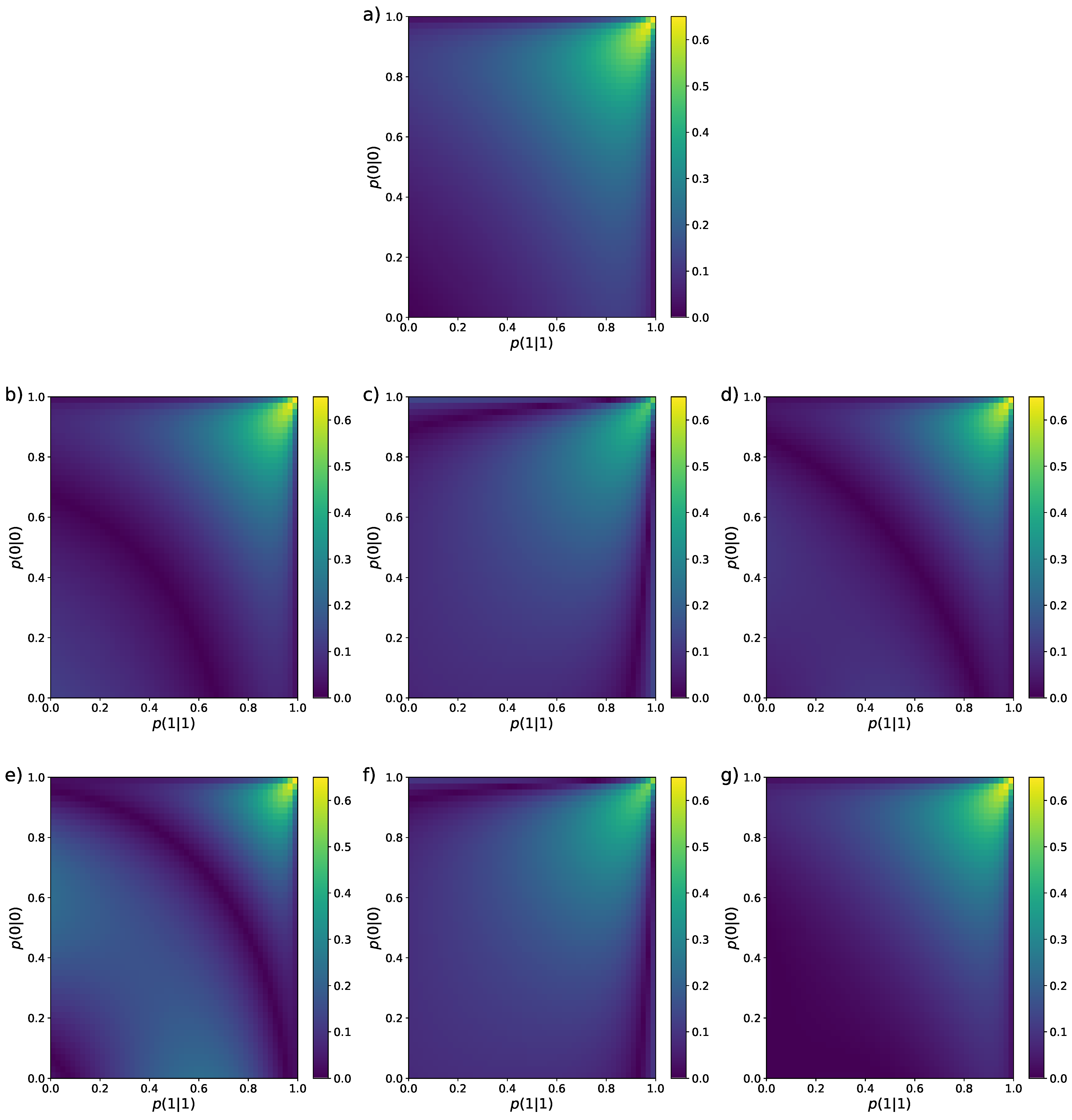
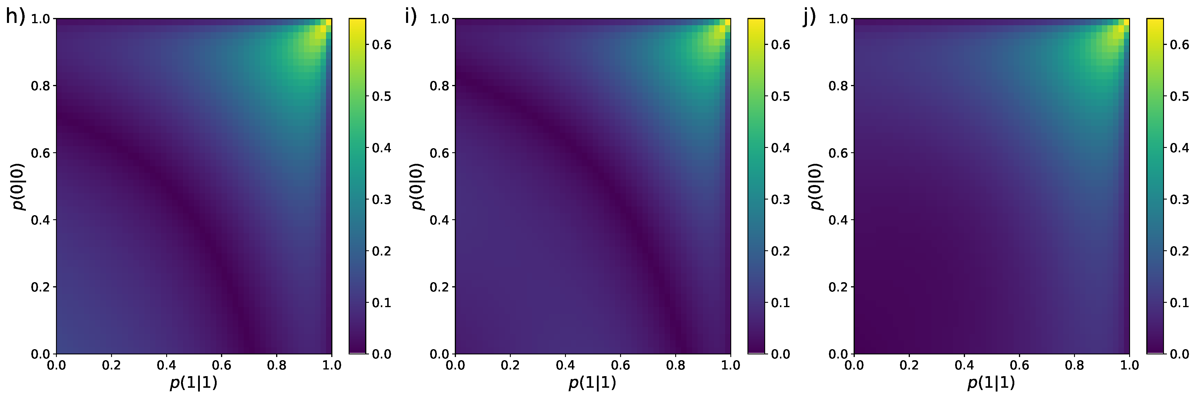
The average value and standard deviation of the different entropy estimators were computed using Equation (5) for $k=1,2$ by generating all $2^N$ possible sequences S and computing the probability of each one using Equation (8), where $p\left(X_1\right)$ are the stationary values given by Equation (36). We have followed this approach to compute the estimator bias $B=\langle \widehat{H}\rangle -H$ and its standard deviation $\sigma =\sqrt{\langle {\widehat{H}}^2\rangle -{\langle \widehat{H}\rangle }^2}$. As an example, we plot the absolute value of the bias for sequences of length $N=4$ in the colour map of Figure 1, for the ten entropy estimators presented in Section 2, as a function of the transition probabilities $p_{00}$ and $p_{11}$.

In Figure 1, we can see that, for all ten estimators, the bias is larger in the region around the values $p_{00}\simeq p_{11}\simeq 1$. The reason is that, in this region, the stationary probabilities of 0 and 1 are very similar, but given these particular values of the transition probabilities, a short sequence will most likely feature only one of these values, which makes it very hard to correctly estimate the entropy in those cases. Apart for this common characteristic, the performance of the estimators when considering only the bias is quite diverse, all of them having different regions where the bias is lowest (darker areas in the panels).

In order to quantitatively compare the performance of the different estimators, we have aggregated all values in the $(p_{00},p_{11})$ plane. We define the aggregated bias of an estimator,

$$\overline{B}={(\Delta p)}^2\sum _{p_{00},p_{11}}\left|B(p_{00},p_{11})\right|,$$

(37)

where the sum runs over all values of the transition probabilities used to produce Figure 1, $\Delta p=0.02$ is the step value used for the grid of the figure, and $B(p_{00},p_{11})$ is the bias for the particular values of the transition probabilities. The aggregated bias given by Equation (37) depends only on the sequence length N.

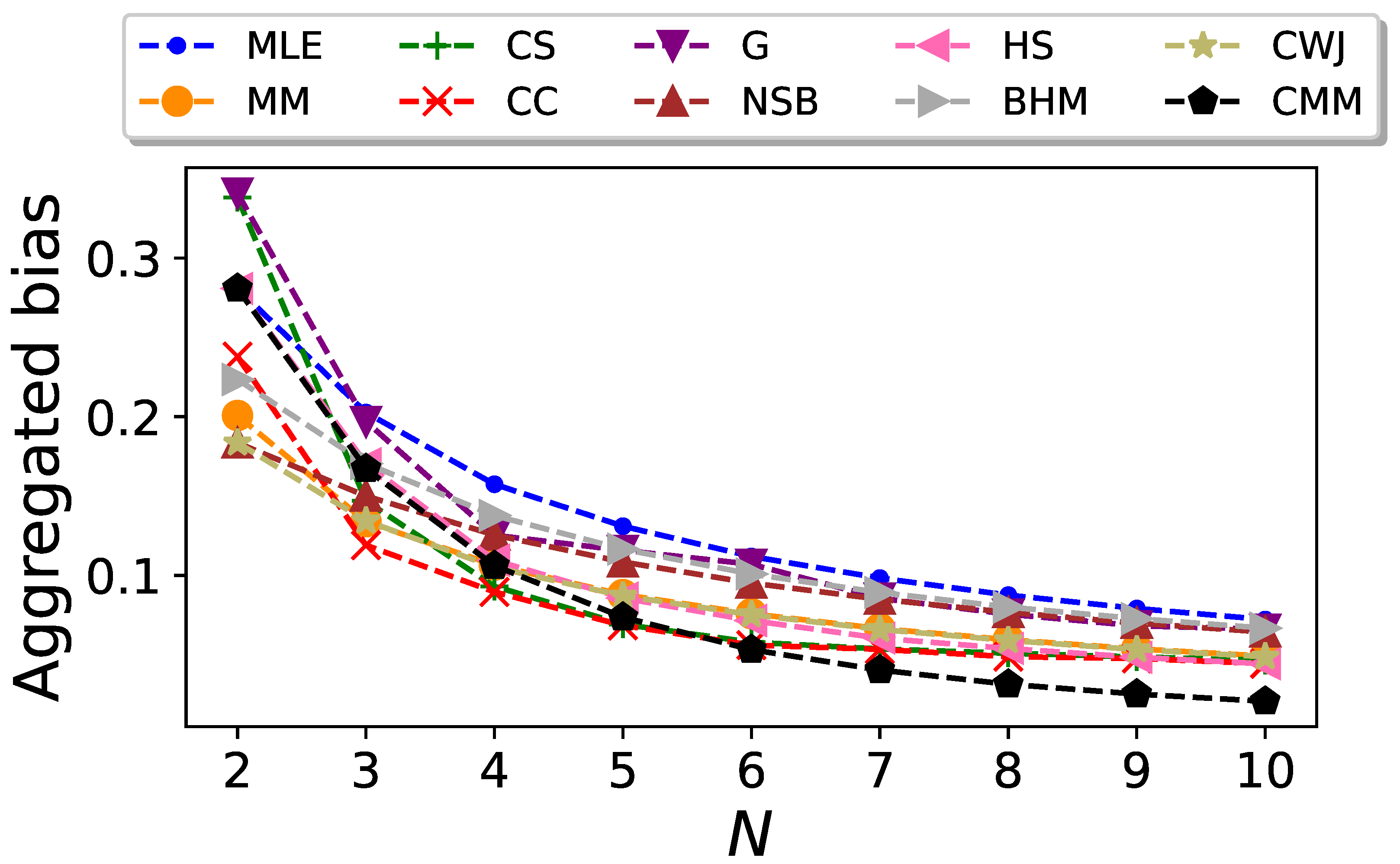
We conduct the previous analysis for different values of N. The resulting plot of the aggregate bias $\overline{B}$ of the entropy estimator as a function of the sequence length is shown in Figure 2. In this figure, we can see that the CC estimator gives the best performance for small values of N, except for $N=2$, where the CWJ estimator has the lowest aggregated bias. However, from $N=7$ it is the CMM estimator which outperforms the rest. The poor performance of this estimator for low values of N is due to the fact that this estimator, in contrast to the others, requires estimating the transition probabilities, as well as the stationary probabilities, and therefore more data are needed. As expected, all the estimators yield an aggregated bias that vanishes as N increases.

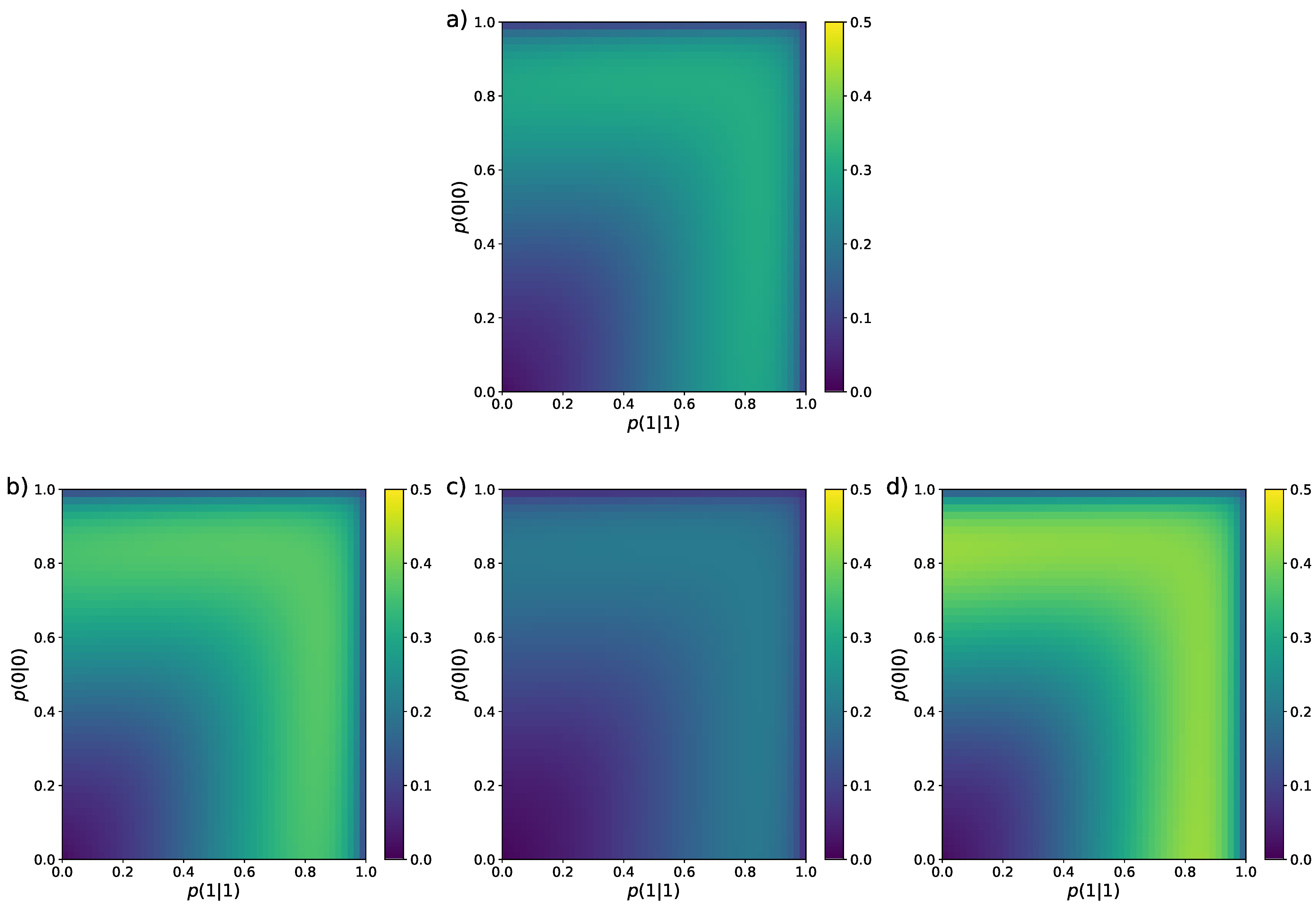
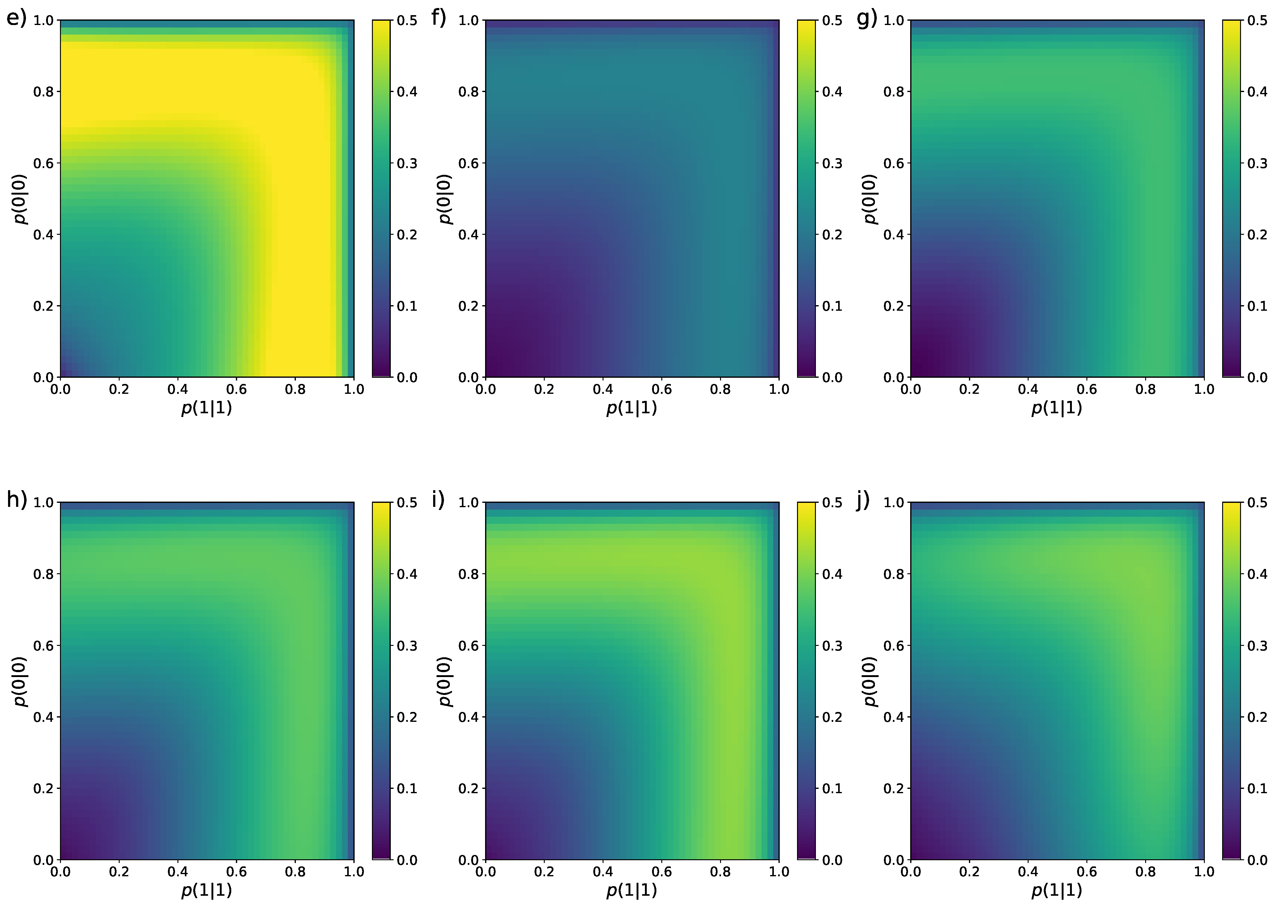
In the colour map of Figure 3, we perform a similar analysis for the standard deviation $\sigma$. In the figure, we find that all ten estimators show a similar structure in the sense that the regions of lowest and highest $\sigma$ are alike. The smallest deviation is mostly located near the left bottom corner of the colour maps and the largest deviation occurs around the regions $(0.65\lesssim p_{00}\lesssim 0.9,0\lesssim p_{11}\lesssim 1)$ and $(0\lesssim p_{00}\lesssim 1,0.65\lesssim p_{11}\lesssim 0.9)$ (green areas in the figures). Of course, the values of $\sigma$ inside these regions vary for each estimator but they all share this similar feature. In this case, by just looking at the colour maps, it is easy to see that BHM (panel f) and NSB (panel c) estimators are the ones with the lowest standard deviation.

The aggregated standard deviation $\overline{\sigma }$, defined in a similar way to the aggregated bias,

$$\overline{\sigma }={(\Delta p)}^2\sum _{p_{00},p_{11}}\sigma (p_{00},p_{11}),$$

(38)

is plotted in Figure 4 as a function of the sequence size N. In agreement with the previous visual test, the BHM and NSB estimators clearly outperform the rest, even though their advantage is less significant as N increases.

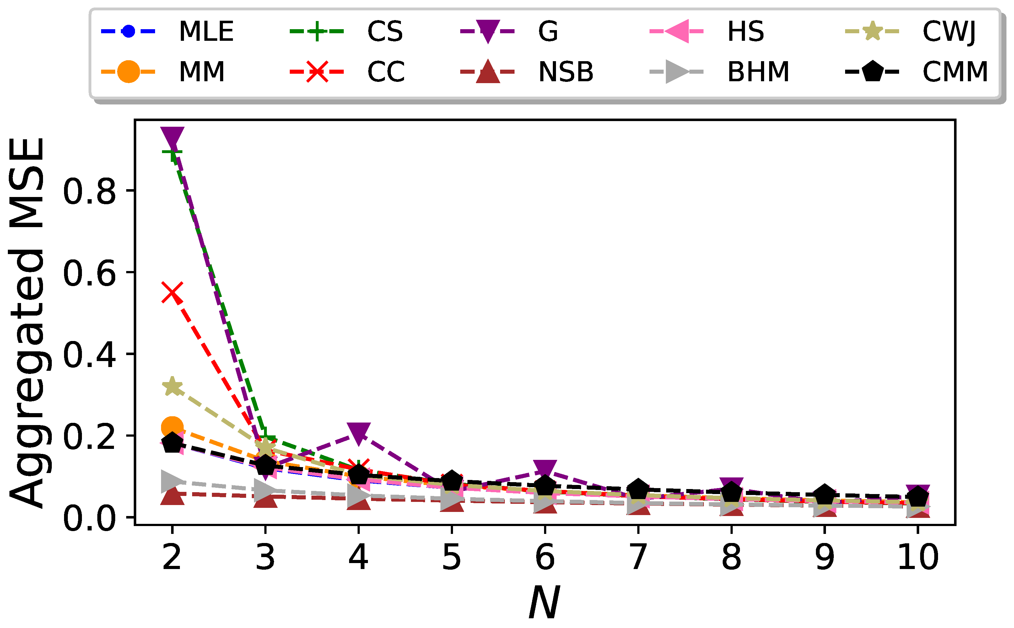
Finally, for every particular N, we compute the mean squared error of the entropy estimators, Equation (4), as a function of $p_{00}$ and $p_{11}$. Its aggregated value

$$\overline{\mathrm{MSE}}={(\Delta p)}^2\sum _{p_{00},p_{11}}\mathrm{MSE}(p_{00},p_{11}),$$

(39)

is plotted as a function of N in Figure 5. Even though the CC and CMM estimators outperform the others when considering only the bias, their large dispersion dominates the mean squared error. Overall, it can be seen that the BHM and NSB estimators surpass the rest when both the bias and standard deviation are considered although, again, their advantage becomes less significant as N increases.

3.2. Undersampled Regime: Block Entropy

Consider a sequence $S=X_1,\dots ,X_N$, where each $X_i=0,1$ is a binary variable, with probabilities $P(X_i=1)=p$, $P(X_i=0)=1-p$. We group the sequence in blocks of size n, such that the jth-block is $B_j=(X_j,\dots ,X_{j+n-1})$. We denote by ${\left\{b_i\right\}}_{i=1,\dots ,2^n}$ the set of all possible blocks. The total number of (overlapping) blocks that can be constructed out of a series of N elements is $N_n=N-n+1$, whereas the total number of possible blocks is $L=2^n$. Hence, depending on the values of n and N, the sequence formed by the $N_n$ blocks, $S_n=B_1,\dots ,B_{N_n}$, will be in an undersampled regime whenever $N_n\ll 2^n$.

The block entropy $H_n$ is defined by

$$H_n=-\sum _{i=1}^{2^n}p\left(b_i\right)ln\left(p\left(b_i\right)\right),$$

(40)

where $p\left(b_i\right)$ is the probability of observing the block $b_i$. The important thing to notice here is that, even if the different outcomes $X_1,\dots ,X_N$ of the binary variable X are independent, the block sequence $B_1,\dots ,B_{N_n}$ obeys a Markov process for $n\ge 2$.

This Markovian property can be easily established by noticing that the block $B_j=(X_j,\dots ,X_{j+n-1})$ can only be followed by the block $B_{j+1}=(X_{j+1},\dots ,X_{j+n-1},1)$ with probability p or by the block $B_{j+1}=(X_{j+1},\dots ,X_{j+n-1},0)$ with probability $1-p$. Therefore, the probability of $B_{j+1}$ depends only on the value of block $B_j$. In Appendix B we show that the dynamics of block sequences in the case that $X_i$ are i.i.d. is equivalent to that of a new stochastic variable Z that can take any of $L=2^n$ possible outcomes, $z_i=0,1,\dots ,2^n-1$, with the following transition probabilities for each state z:

$$p\left(z_k\right|z_i)=\left\{\begin{array}{cc}1-p,\hfill & \mathrm{if}{z}_k=2z_i\left(\mathrm{mod}{2}^n\right),\hfill \\ p,\hfill & \mathrm{if}{z}_k=2z_i\left(\mathrm{mod}{2}^n\right)+1,\hfill \\ 0,\hfill & \mathrm{otherwise}.\hfill \end{array}\right.$$

(41)

These types of Markovian systems have been related to Linguistics and Zipf’s law [25].

The previous result can be generalized. If the original sequence $X_1,\dots ,X_N$ is Markovian of order $m\ge 1$, then the dynamics of the block sequences $B_1,\dots ,B_{N_n}$ are also Markovian of order 1, for $n\ge m$.

It is well known [5] that the block entropy, when the original sequence S is constructed out of i.i.d. binary variables, obeys

$$H_n=n{H}_1,$$

(42)

where $H_1$ can be calculated using Equation (35) with $p\left(1\right)=p$ and $p\left(0\right)=1-p$. Therefore, the entropy rate is constant.

We want to compare now the performance of the different estimators defined before when computing the block entropy. In this case, we cannot use an expression equivalent to Equation (5), summing over all sequences $S_n$, since the number of possible sequences is ${\left(2^n\right)}^{N_n}$, and it is not possible to enumerate all the sequences even for relatively small values of n and $N_n$. As an example, we employ in our numerical study $N_n=20$ and $n=6$, for which the total number of possible sequences is $2^{120}$. Therefore, we use the sample mean ${\mu }_M\left[{\widehat{H}}_n\right]$ and the sample variance $s_M^2\left[{\widehat{H}}_n\right]$ as unbiased estimators to the expected value $\langle {\widehat{H}}_n\rangle$ and the variance ${\sigma }^2\left[{\widehat{H}}_n\right]$, respectively. After generating a sample of M independent sequences $S_n^i$, $i=1,\dots ,M$, and computing the estimator ${\widehat{H}}_n\left(S_n^i\right)$ for each of the sequences, those statistics are computed as

$$\begin{array}{cc}\hfill {\mu }_M\left[{\widehat{H}}_n\right]& ={\displaystyle \frac{1}{M}}\sum _{i=1}^M{\widehat{H}}_n\left(S_n^i\right),\hfill \\ \hfill s_M^2\left[{\widehat{H}}_n\right]& =\frac{1}{M-1}\sum _{i=1}^M{({\widehat{H}}_n\left(S_n^i\right)-{\mu }_M\left[{\widehat{H}}_n\right])}^2.\hfill \end{array}$$

(43)

Using Equations (42) and (43) we can calculate the bias $B_n={\mu }_M\left[{\widehat{H}}_n\right]-H_n$, the standard deviation $s_M\left[{\widehat{H}}_n\right]$, and the mean squared error $s_M^2\left[{\widehat{H}}_n\right]+B_n^2$. In the following, we set $M={10}^4$ for our simulations.

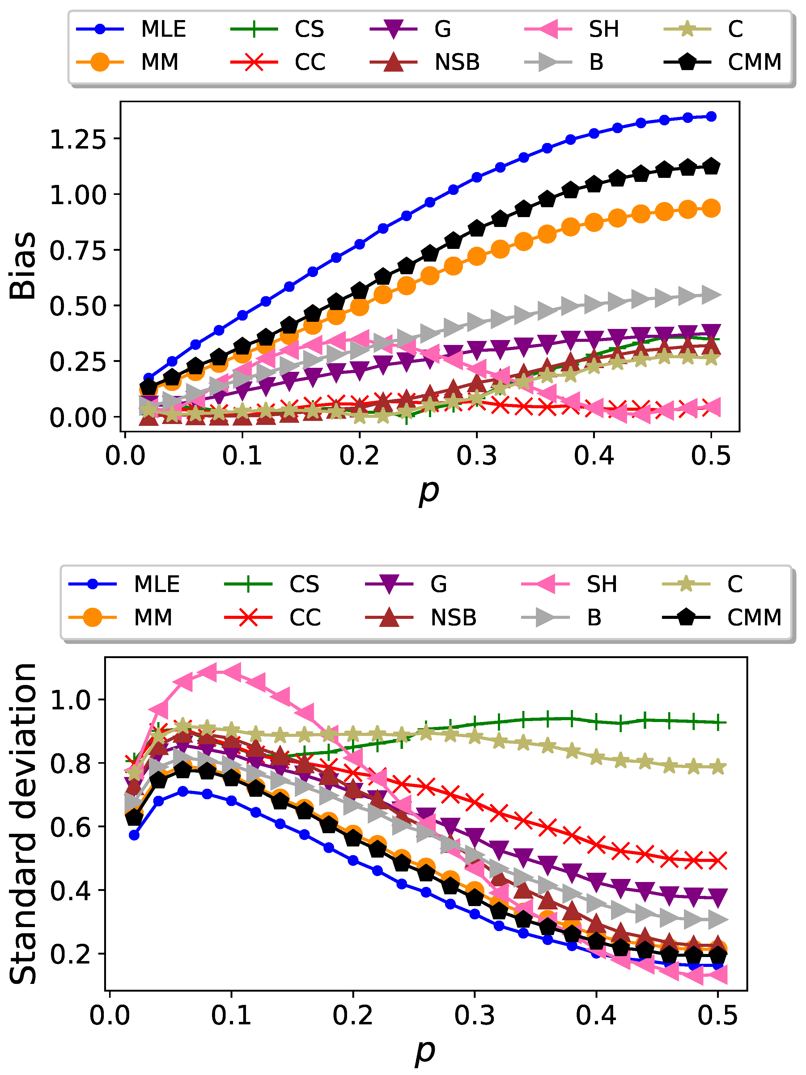
In Figure 6, we show plots of $B_n$ and $s_M\left[{\widehat{H}}_n\right]$ as a function of p ranging from $0.02$ to $0.5$ with step $\Delta p=0.02$, for $N_n=20$. We find that the CC estimator performs remarkably well in terms of bias and we highlight its robustness. Unlike the other estimators, which display significant variations in their bias as p changes, the CC estimator remains approximately constant at a low value. However, the CC estimator presents a high standard deviation, whereas the MLE and MM exhibit the lowest standard deviation. For the majority of estimators considered, we observe that the ones with higher bias are the ones with lower deviation. An exception is the HS estimator.

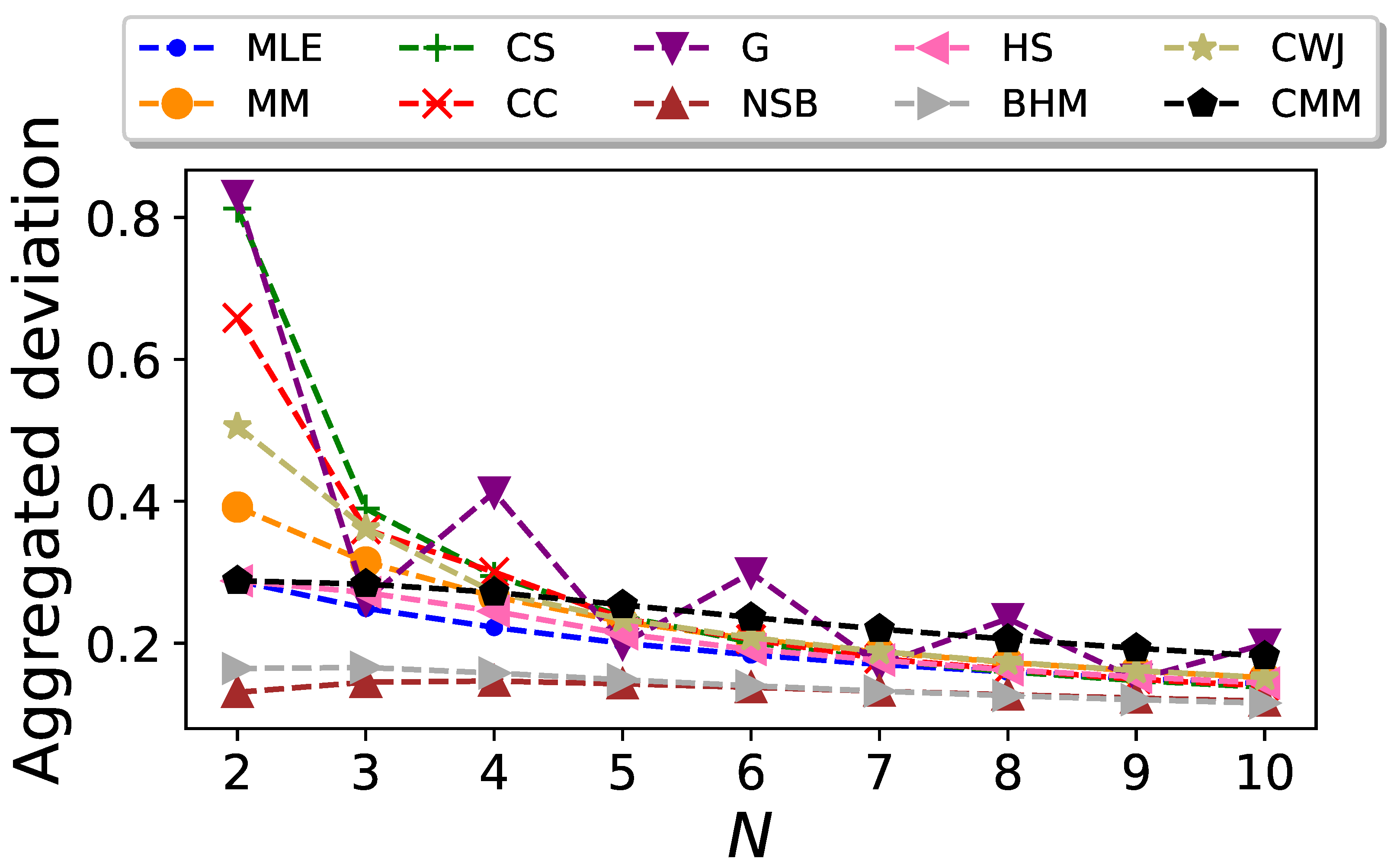
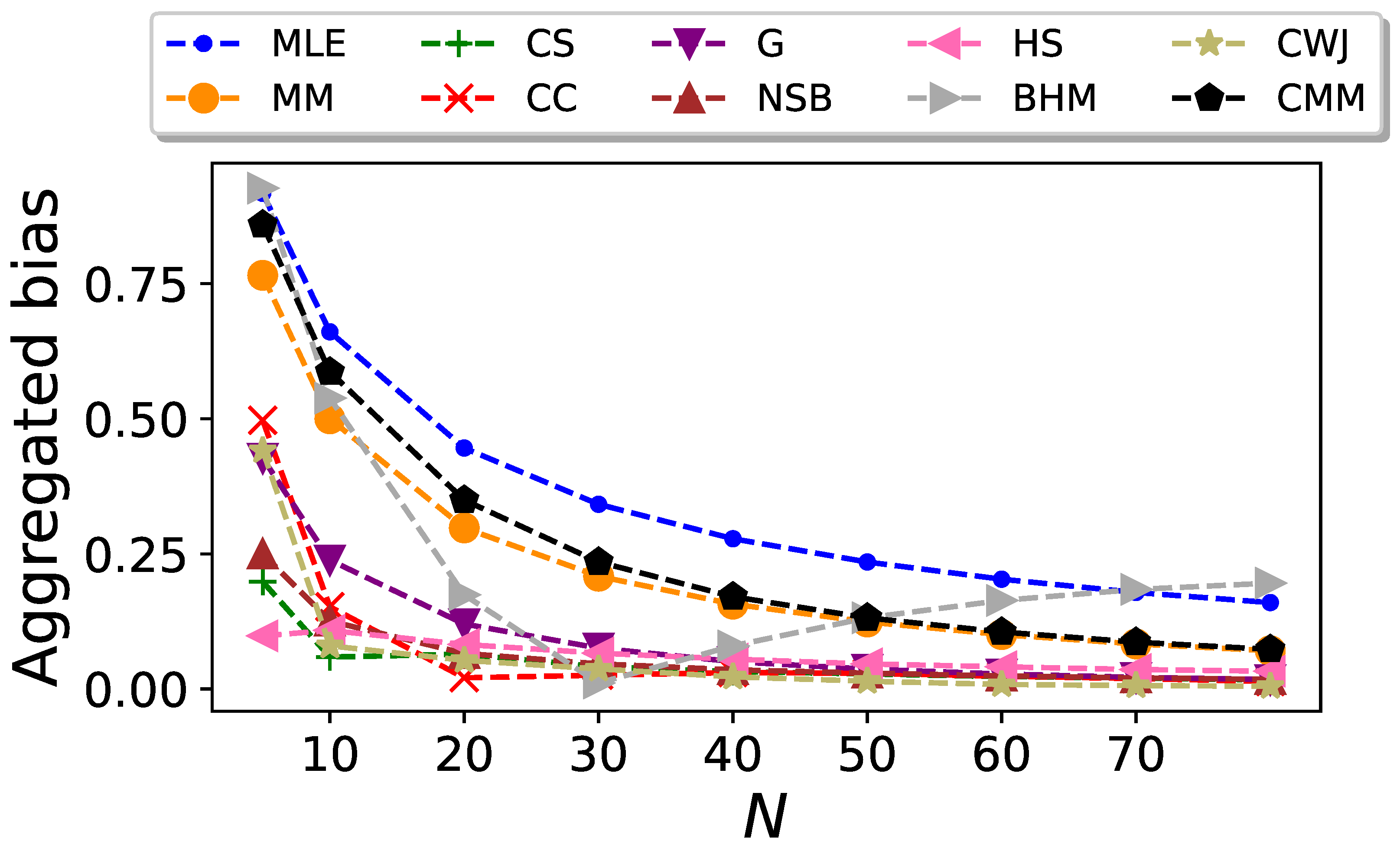
To analyze the changes in the overall performances of the estimators with different values of N, we calculated the aggregated bias as

$${\overline{B}}_n=\Delta p\sum _p\left|B_n\left(p\right)\right|.$$

(44)

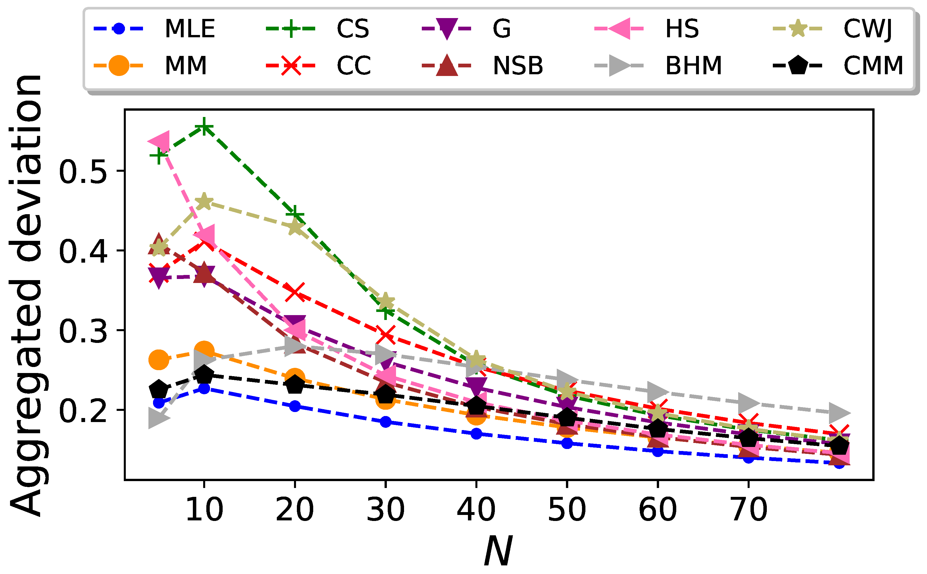
Similarly, we calculated the aggregated standard deviation as

$${\overline{s}}_n=\Delta p\sum _p{s}_M\left[{\widehat{H}}_n\right]\left(p\right),$$

(45)

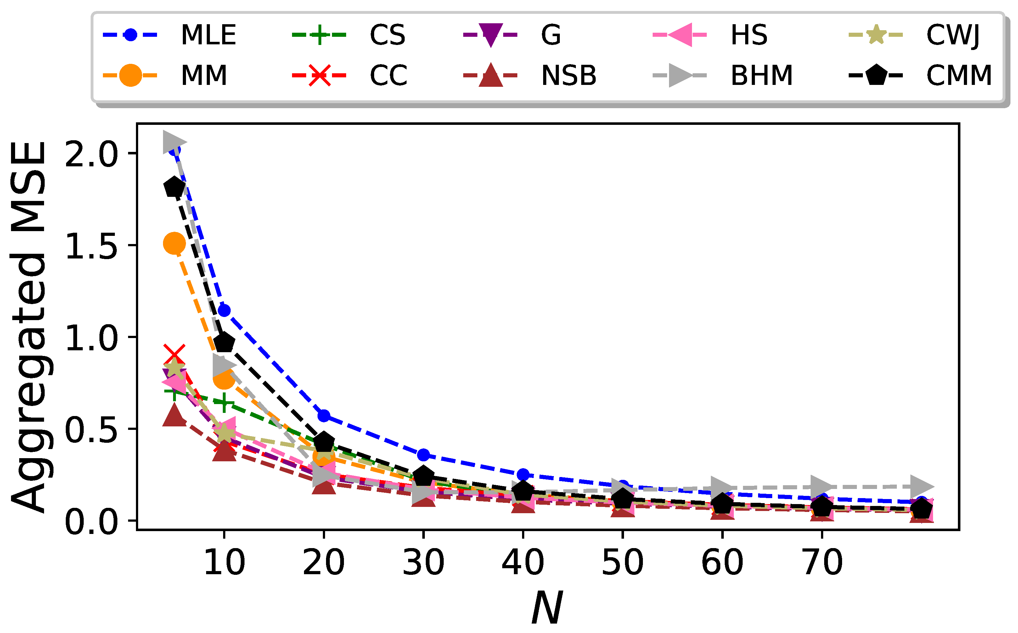
and the aggregated mean squared error as

$${\overline{\mathrm{MSE}}}_n=\Delta p\sum _p(s_M^2\left[{\widehat{H}}_n\right]\left(p\right)+B_n{\left(p\right)}^2).$$

(46)

The resulting plots are shown in Figure 7, Figure 8 and Figure 9, respectively.

It was expected that the total bias of the estimators would decrease by increasing N, and in Figure 7 it can be seen that this is indeed the case for all estimators except for the BHM estimator. Surprisingly, the bias of this estimator follows a typical pattern of decreasing as the sample size increases, just like the other estimators. However, it takes an unexpected turn starting at $N=20$, as it begins to increase once more. A possible reason for this behaviour is that the BHM estimator is designed to minimize the MSE.

Similarly to the results obtained for the binary Markovian case, the CC estimator demonstrates in Figure 7 excellent performance when solely evaluating bias. Even though its performance for a data size of $N=5$ is not outstanding, it begins to outperform all but the CS, CWJ, and HS estimators starting at $N=10$, and from that point onward, the CC estimator consistently ranks among the top-performing estimators, together with the NSB and CWJ estimators.

By comparing Figure 7 and Figure 8, it can be seen that there is a certain balance: An estimator with a higher bias usually has a lower deviation when compared to others. This is clearly the case for the MLE and MM estimators, as they are the two with the worst performances in terms of bias, but they have the lowest aggregated standard deviation for most of the data sizes considered.

In this interplay between bias and standard deviation observed for most of the entropy estimators considered here, the NSB estimator is the one that presents the best performance when considering both statistics. From Figure 9, it is clear that this estimator shows the lowest aggregated mean squared error, although just from $N=20$ the difference with other estimators like the CC or the G becomes vanishingly small.

It can be seen in Figure 7, Figure 8 and Figure 9 that the performance of the CMM estimator is very similar to MM’s performance, especially for large values of N. This suggests that for Markovian systems defined by the transition probabilities given by Equation (41), the correction introduced in Equation (34) is not significant, particularly in the limit of large N.

4. Discussion

We have made a detailed comparison of nine of the most widely used entropy estimators when applied to Markovian sequences. We have also included in this analysis a new proposed estimator, motivated by the results presented in ref. [34]. One crucial difference in the way these estimators are constructed is that only the correlation coverage-adjusted estimator [27] and the corrected Miller–Madow estimator take into account the order in which the elements appear in the sequence. To calculate the CC estimator, it is necessary to know the entire history of the sequence, and the computation of the CMM estimator requires the calculation of the transition probabilities. On the contrary, for all other estimators, it is sufficient to know the number of times that each element is present in the sequence, independently of the position in which they appear. Remarkably, this novel approach to the issue of entropy estimation allows us to reduce the bias, even in undersampled regimes. Unfortunately, both of these estimators present large dispersion, which reduces their overall quality.

We have found that, when dealing with Markovian sequences, on average, the Nemenman–Shafee–Bialek estimator [54,55,56] outperforms the rest when taking into account both the bias and the standard deviation for both analyzed cases, namely, binary sequences and an undersampled regime. Ref. [16] presented a similar analysis but for uniformly distributed sequences of bytes and bites, and concluded that the estimator with the lowest mean squared error was the Shrinkage estimator [20]. Hence, when choosing a reliable estimator, it is not only important to consider the amount of data available, but also whether correlations might be present in the sequence.

Further analyses should consider Markovian sequences of higher order [63,64]. Another interesting topic would be systems described with continuous variables [65,66], where the presence of noise is particularly important. Finally, we stress that there are alternative entropies not considered here [67], for which the existence of accurate estimators is still an open question. Finally, an exciting possibility would be a comparative study of estimators valid for more than one random variable or probability distributions, leading, respectively, to mutual information [68,69] and relative entropy [47,70,71].

References

- Lewontin, R.C. The Apportionment of Human Diversity. In Evolutionary Biology: Volume 6; Dobzhansky, T., Hecht, M.K., Steere, W.C., Eds.; Springer: New York, NY, USA, 1972; pp. 381–398. [Google Scholar] [CrossRef]
- Stinson, D.R. Cryptography: Theory and Practice, 1st ed.; CRC Press Inc.: Boca Raton, FL, USA, 1995. [Google Scholar]
- Strong, S.P.; Koberle, R.; de Ruyter van Steveninck, R.R.; Bialek, W. Entropy and Information in Neural Spike Trains. Phys. Rev. Lett. 1998, 80, 197–200. [Google Scholar] [CrossRef]
- Yeo, G.; Burge, C. Maximum Entropy Modeling of Short Sequence Motifs with Applications to RNA Splicing Signals. J. Comput. Biol. J. Comput. Mol. Cell Biol. 2004, 11, 377–394. [Google Scholar] [CrossRef] [PubMed]
- Cover, T.; Thomas, J. Elements of Information Theory; John Wiley and Sons: Hoboken, NJ, USA, 2006. [Google Scholar]
- Letellier, C. Estimating the Shannon Entropy: Recurrence Plots versus Symbolic Dynamics. Phys. Rev. Lett. 2006, 96, 254102. [Google Scholar] [CrossRef]
- Victor, J. Approaches to Information-Theoretic Analysis of Neural Activity. Biol. Theory 2006, 1, 302–316. [Google Scholar] [CrossRef] [PubMed]
- Hlaváčková-Schindler, K.; Paluš, M.; Vejmelka, M.; Bhattacharya, J. Causality detection based on information-theoretic approaches in time series analysis. Phys. Rep. 2007, 441, 1–46. [Google Scholar] [CrossRef]
- Rosso, O.A.; Larrondo, H.A.; Martin, M.T.; Plastino, A.; Fuentes, M.A. Distinguishing Noise from Chaos. Phys. Rev. Lett. 2007, 99, 154102. [Google Scholar] [CrossRef]
- Sherwin, W.B. Entropy and Information Approaches to Genetic Diversity and its Expression: Genomic Geography. Entropy 2010, 12, 1765–1798. [Google Scholar] [CrossRef]
- Zanin, M.; Zunino, L.; Rosso, O.A.; Papo, D. Permutation Entropy and Its Main Biomedical and Econophysics Applications: A Review. Entropy 2012, 14, 1553–1577. [Google Scholar] [CrossRef]
- Bentz, C.; Alikaniotis, D.; Cysouw, M.; Ferrer-i Cancho, R. The Entropy of Words—Learnability and Expressivity across More than 1000 Languages. Entropy 2017, 19, 275. [Google Scholar] [CrossRef]
- Cassetti, J.; Delgadino, D.; Rey, A.; Frery, A.C. Entropy Estimators in SAR Image Classification. Entropy 2022, 24, 509. [Google Scholar] [CrossRef]
- Shannon, C.E. A Mathematical Theory of Communication. Bell Syst. Tech. J. 1948, 27, 379–423. [Google Scholar] [CrossRef]
- Paninski, L. Estimation of Entropy and Mutual Information. Neural Comput. 2003, 15, 1191–1253. [Google Scholar] [CrossRef]
- Contreras Rodríguez, L.; Madarro-Capó, E.J.; Legón-Pérez, C.M.; Rojas, O.; Sosa-Gómez, G. Selecting an Effective Entropy Estimator for Short Sequences of Bits and Bytes with Maximum Entropy. Entropy 2021, 23, 561. [Google Scholar] [CrossRef]
- Levina, A.; Priesemann, V.; Zierenberg, J. Tackling the subsampling problem to infer collective properties from limited data. Nat. Rev. Phys. 2022, 4, 770–784. [Google Scholar] [CrossRef]
- Chao, A.; Shen, T.J. Nonparametric estimation of Shannon’s diversity index when there are unseen species in sample. Environ. Ecol. Stat. 2003, 10, 429–443. [Google Scholar] [CrossRef]
- Vu, V.Q.; Yu, B.; Kass, R.E. Coverage-adjusted entropy estimation. In Statistics in Medicine; John Wiley & Sons, Ltd.: Hoboken, NJ, USA, 2007; Volume 26, pp. 4039–4060. [Google Scholar] [CrossRef]
- Hausser, J.; Strimmer, K. Entropy Inference and the James-Stein Estimator, with Application to Nonlinear Gene Association Networks. J. Mach. Learn. Res. 2009, 10, 1469–1484. [Google Scholar]
- Arora, A.; Meister, C.; Cotterell, R. Estimating the Entropy of Linguistic Distributions. In Proceedings of the 60th Annual Meeting of the Association for Computational Linguistics (Volume 2: Short Papers), Dublin, Ireland, 22–27 May 2022; Association for Computational Linguistics: Cedarville, OH, USA, 2022; pp. 175–195. [Google Scholar] [CrossRef]
- Gardiner, C.W. Handbook of Stochastic Methods for Physics, Chemistry and the Natural Sciences; Springer: Berlin/Heidelberg, Germany, 1965. [Google Scholar]
- Churchill, G.A. Stochastic models for heterogeneous DNA sequences. Bull. Math. Biol. 1989, 51, 79–94. [Google Scholar] [CrossRef]
- Wilks, D.S.; Wilby, R.L. The weather generation game: A review of stochastic weather models. Prog. Phys. Geogr. Earth Environ. 1999, 23, 329–357. [Google Scholar] [CrossRef]
- Kanter, I.; Kessler, D.A. Markov Processes: Linguistics and Zipf’s Law. Phys. Rev. Lett. 1995, 74, 4559–4562. [Google Scholar] [CrossRef]
- Crutchfield, J.P.; Feldman, D.P. Regularities unseen, randomness observed: Levels of entropy convergence. Chaos Interdiscip. J. Nonlinear Sci. 2003, 13, 25–54. [Google Scholar] [CrossRef]
- De Gregorio, J.; Sánchez, D.; Toral, R. An improved estimator of Shannon entropy with applications to systems with memory. Chaos Solitons Fractals 2022, 165, 112797. [Google Scholar] [CrossRef]
- Yulmetyev, R.M.; Demin, S.A.; Panischev, O.Y.; Hänggi, P.; Timashev, S.F.; Vstovsky, G.V. Regular and stochastic behavior of Parkinsonian pathological tremor signals. Phys. Stat. Mech. Appl. 2006, 369, 655–678. [Google Scholar] [CrossRef]
- Ho, D.T.; Cao, T.H. A high-order hidden Markov model for emotion detection from textual data. In Pacific Rim Knowledge Acquisition Workshop; Springer: Berlin/Heidelberg, Germany, 2012; pp. 94–105. [Google Scholar]
- Seifert, M.; Gohr, A.; Strickert, M.; Grosse, I. Parsimonious higher-order hidden Markov models for improved array-CGH analysis with applications to Arabidopsis Thaliana. PLoS Comput. Biol. 2012, 8, e1002286. [Google Scholar] [CrossRef]
- Singer, P.; Helic, D.; Taraghi, B.; Strohmaier, M. Detecting memory and structure in human navigation patterns using Markov chain models of varying order. PLoS ONE 2014, 9, e102070. [Google Scholar] [CrossRef] [PubMed]
- Meyer, H.; Rieger, H. Optimal Non-Markovian Search Strategies with n-Step Memory. Phys. Rev. Lett. 2021, 127, 070601. [Google Scholar] [CrossRef]
- Wilson Kemsley, S.; Osborn, T.J.; Dorling, S.R.; Wallace, C.; Parker, J. Selecting Markov chain orders for generating daily precipitation series across different Köppen climate regimes. Int. J. Climatol. 2021, 41, 6223–6237. [Google Scholar] [CrossRef]
- Weiß, C.H. Measures of Dispersion and Serial Dependence in Categorical Time Series. Econometrics 2019, 7, 17. [Google Scholar] [CrossRef]
- Wang, Y.; Yang, Z. On a Markov multinomial distribution. Math. Sci. 1995, 20, 40–49. [Google Scholar]
- Grassberger, P. Entropy Estimates from Insufficient Samplings. arXiv 2008, arXiv:2301.13647. [Google Scholar] [CrossRef]
- Bonachela, J.A.; Hinrichsen, H.; Muñoz, M.A. Entropy estimates of small data sets. J. Phys. Math. Theor. 2008, 41, 202001. [Google Scholar] [CrossRef]
- Bhat, U.N.; Lal, R. Number of successes in Markov trials. Adv. Appl. Probab. 1988, 20, 677–680. [Google Scholar] [CrossRef]
- Burnham, K.P.; Overton, W.S. Estimation of the size of a closed population when capture probabilities vary among animals. Biometrika 1978, 65, 625–633. [Google Scholar] [CrossRef]
- Wolpert, D.H.; Wolf, D.R. Estimating functions of probability distributions from a finite set of samples. Phys. Rev. E 1995, 52, 6841–6854. [Google Scholar] [CrossRef] [PubMed]
- Vinck, M.; Battaglia, F.P.; Balakirsky, V.B.; Vinck, A.J.H.; Pennartz, C.M.A. Estimation of the entropy based on its polynomial representation. Phys. Rev. E 2012, 85, 051139. [Google Scholar] [CrossRef]
- Zhang, Z. Entropy Estimation in Turing’s Perspective. Neural Comput. 2012, 24, 1368–1389. [Google Scholar] [CrossRef] [PubMed]
- Archer, E.W.; Park, I.M.; Pillow, J.W. Bayesian entropy estimation for binary spike train data using parametric prior knowledge. In Advances in Neural Information Processing Systems; Burges, C., Bottou, L., Welling, M., Ghahramani, Z., Weinberger, K., Eds.; Curran Associates, Inc.: Red Hook, NY, USA, 2013; Volume 26. [Google Scholar]
- Wolpert, D.H.; DeDeo, S. Estimating Functions of Distributions Defined over Spaces of Unknown Size. Entropy 2013, 15, 4668–4699. [Google Scholar] [CrossRef]
- Valiant, G.; Valiant, P. Estimating the Unseen: Improved Estimators for Entropy and Other Properties. Assoc. Comput. Mach. 2017, 64, 41. [Google Scholar] [CrossRef]
- Grassberger, P. On Generalized Schürmann Entropy Estimators. Entropy 2022, 24, 680. [Google Scholar] [CrossRef]
- Piga, A.; Font-Pomarol, L.; Sales-Pardo, M.; Guimerà, R. Bayesian estimation of information-theoretic metrics for sparsely sampled distributions. arXiv 2023, arXiv:2301.13647. [Google Scholar] [CrossRef]
- Miller, G. Note on the bias of information estimates. Inf. Theory Psychol. Probl. Methods 1955, 71, 108. [Google Scholar]
- Schürmann, T. Bias analysis in entropy estimation. J. Phys. Math. Gen. 2004, 37, L295–L301. [Google Scholar] [CrossRef]
- Trybula, S. Some Problems of Simultaneous Minimax Estimation. Ann. Math. Stat. 1958, 29, 245–253. [Google Scholar] [CrossRef]
- Krichevsky, R.; Trofimov, V. The performance of universal encoding. IEEE Trans. Inf. Theory 1981, 27, 199–207. [Google Scholar] [CrossRef]
- Schürmann, T.; Grassberger, P. Entropy estimation of symbol sequences. Chaos Interdiscip. J. Nonlinear Sci. 1996, 6, 414–427. [Google Scholar] [CrossRef]
- Holste, D.; Große, I.; Herzel, H. Bayes’ estimators of generalized entropies. J. Phys. Math. Gen. 1998, 31, 2551. [Google Scholar] [CrossRef]
- Nemenman, I.; Shafee, F.; Bialek, W. Entropy and Inference, Revisited. In Advances in Neural Information Processing Systems; Dietterich, T., Becker, S., Ghahramani, Z., Eds.; MIT Press: Cambridge, MA, USA, 2001; Volume 14. [Google Scholar]
- Nemenman, I.; Bialek, W.; de Ruyter van Steveninck, R. Entropy and information in neural spike trains: Progress on the sampling problem. Phys. Rev. E 2004, 69, 056111. [Google Scholar] [CrossRef] [PubMed]
- Nemenman, I. Coincidences and Estimation of Entropies of Random Variables with Large Cardinalities. Entropy 2011, 13, 2013–2023. [Google Scholar] [CrossRef]
- Simomarsili. ndd—Bayesian Entropy Estimation from Discrete Data. 2021. Available online: https://github.com/simomarsili/ndd (accessed on 30 October 2023).
- Horvitz, D.G.; Thompson, D.J. A Generalization of Sampling without Replacement from a Finite Universe. J. Am. Stat. Assoc. 1952, 47, 663–685. [Google Scholar] [CrossRef]
- Rényi, A. On measures of entropy and information. In Proceedings of the Fourth Berkeley Symposium on Mathematical Statistics Probability, Oakland, CA, USA, 20–30 July 1961; University of California Press: Oakland, CA, USA, 1961; Volume 1, pp. 547–561. [Google Scholar]
- Gruber, M.H.J. Improving Efficiency by Shrinkage: The James-Stein and Ridge Regression Estimators; Routledge: London, UK, 1998. [Google Scholar]
- Schäfer, J.; Strimmer, K. A Shrinkage Approach to Large-Scale Covariance Matrix Estimation and Implications for Functional Genomics. Stat. Appl. Genet. Mol. Biol. 2005, 4, 32. [Google Scholar] [CrossRef]
- Chao, A.; Wang, Y.T.; Jost, L. Entropy and the species accumulation curve: A novel entropy estimator via discovery rates of new species. Methods Ecol. Evol. 2013, 4, 1091–1100. [Google Scholar] [CrossRef]
- Raftery, A.E. A model for high-order Markov chains. J. R. Stat. Soc. Ser. Stat. Methodol. 1985, 47, 528–539. [Google Scholar] [CrossRef]
- Strelioff, C.C.; Crutchfield, J.P.; Hübler, A.W. Inferring Markov chains: Bayesian estimation, model comparison, entropy rate, and out-of-class modeling. Phys. Rev. E 2007, 76, 011106. [Google Scholar] [CrossRef] [PubMed]
- Bercher, J.F.; Vignat, C. Estimating the entropy of a signal with applications. IEEE Trans. Signal Process. 2000, 48, 1687–1694. [Google Scholar] [CrossRef]
- Feutrill, A.; Roughan, M. A review of Shannon and differential entropy rate estimation. Entropy 2021, 23, 1046. [Google Scholar] [CrossRef]
- Beck, C. Generalised information and entropy measures in physics. Contemp. Phys. 2009, 50, 495–510. [Google Scholar] [CrossRef]
- Kraskov, A.; Stögbauer, H.; Grassberger, P. Estimating mutual information. Phys. Rev. E 2004, 69, 066138. [Google Scholar] [CrossRef]
- Walters-Williams, J.; Li, Y. Estimation of mutual information: A survey. In Proceedings of the Rough Sets and Knowledge Technology: 4th International Conference, RSKT 2009, Gold Coast, Australia, 14–16 July 2009; Proceedings 4. Springer: Berlin/Heidelberg, Germany, 2009; pp. 389–396. [Google Scholar]
- Minculete, N.; Savin, D. Some properties of a type of the entropy of an ideal and the divergence of two ideals. arXiv 2023, arXiv:2305.07975. [Google Scholar] [CrossRef]
- Camaglia, F.; Nemenman, I.; Mora, T.; Walczak, A.M. Bayesian estimation of the Kullback-Leibler divergence for categorical sytems using mixtures of Dirichlet priors. arXiv 2023, arXiv:2307.04201. [Google Scholar] [CrossRef]
- Montgomery-Smith, S.; Schürmann, T. Unbiased Estimators for Entropy and Class Number. arXiv 2014, arXiv:1410.5002. [Google Scholar] [CrossRef]
- Good, I. The population frequencies of species and the estimation of population parameters. Biometrika 1953, 40, 237–264. [Google Scholar] [CrossRef]
Figure 1.
Colour maps representing the bias of the nine entropy estimators reviewed in Section 2 for Markovian binary sequences of length . The values of the transition probabilities and vary from to with step . (a) MLE [Equation (12)], (b) Miller–Madow [48], (c) Nemenman et al. [54], (d) Chao–Shen [18], (e) Grassberger [36], (f) Bonachela et al. [37], (g) Shrinkage [20], (h) Chao et al. [62], (i) correlation coverage-adjusted [27], (j) corrected Miller–Madow [Equation (34)].
Figure 2.
Aggregated bias of the entropy estimators for Markovian binary sequences as a function of the sequence size N.
Figure 3.
Colour maps representing the standard deviation of the nine entropy estimators reviewed in Section 2 for Markovian binary sequences of length . The values of the transition probabilities and vary from to with step . (a) MLE [Equation (12)], (b) Miller–Madow [48], (c) Nemenman et al. [54], (d) Chao–Shen [18], (e) Grassberger [36], (f) Bonachela et al. [37], (g) Shrinkage [20], (h) Chao et al. [62], (i) correlation coverage-adjusted [27], (j) corrected Miller–Madow [Equation (34)].
Figure 4.
Aggregated standard deviation of the entropy estimators for Markovian binary sequences as a function of the sequence size N.
Figure 5.
Aggregated mean squared error of the entropy estimators for Markovian binary sequences as a function of the sequence size N.
Figure 6.
Bias (top) and standard deviation (bottom) of the entropy estimators, when applied to Markovian sequences of length and , generated from the transition probabilities given by Equation (41), as functions of p, which vary from to with step . By construction, the plot is symmetric around .
Figure 7.
Aggregated bias of the entropy estimators for Markovian sequences in the undersampled regime with , generated from the transition probabilities given by Equation (41), as a function of the sequence size N.
Figure 8.
Aggregated standard deviation of the entropy estimators for Markovian sequences in the undersampled regime with , generated from the transition probabilities given by Equation (41), as a function of the sequence size N.
Figure 9.
Aggregated mean squared error of the entropy estimators for Markovian sequences in the undersampled regime with , generated from the transition probabilities given by Equation (41), as a function of the sequence size N.
Disclaimer/Publisher’s Note: The statements, opinions and data contained in all publications are solely those of the individual author(s) and contributor(s) and not of MDPI and/or the editor(s). MDPI and/or the editor(s) disclaim responsibility for any injury to people or property resulting from any ideas, methods, instructions or products referred to in the content. |
© 2024 by the authors. Licensee MDPI, Basel, Switzerland. This article is an open access article distributed under the terms and conditions of the Creative Commons Attribution (CC BY) license (https://creativecommons.org/licenses/by/4.0/).
Share and Cite
MDPI and ACS Style
De Gregorio, J.; Sánchez, D.; Toral, R. Entropy Estimators for Markovian Sequences: A Comparative Analysis. Entropy 2024, 26, 79. https://doi.org/10.3390/e26010079
AMA Style
De Gregorio J, Sánchez D, Toral R. Entropy Estimators for Markovian Sequences: A Comparative Analysis. Entropy. 2024; 26(1):79. https://doi.org/10.3390/e26010079
Chicago/Turabian StyleDe Gregorio, Juan, David Sánchez, and Raúl Toral. 2024. "Entropy Estimators for Markovian Sequences: A Comparative Analysis" Entropy 26, no. 1: 79. https://doi.org/10.3390/e26010079
Note that from the first issue of 2016, this journal uses article numbers instead of page numbers. See further details here.