
Bulk Operator Reconstruction in Topological Tensor Network and Generalized Free Fields

1
State Key Laboratory of Surface Physics, Fudan University, Shanghai 200433, China
2
Department of Physics and Center for Field Theory and Particle Physics, Fudan University, Shanghai 200433, China
3
Institute for Nanoelectronic Devices and Quantum Computing, Fudan University, Shanghai 200433, China
4
Yau Mathematical Sciences Center, Tsinghua University, Beijing 100084, China
5
Yanqi Lake Beijing Institute of Mathematical Sciences and Applications (BIMSA), Huairou District, Beijing 101408, China
*
Author to whom correspondence should be addressed.
Entropy 2023, 25(11), 1543; https://doi.org/10.3390/e25111543
Submission received: 16 October 2023
/
Revised: 10 November 2023
/
Accepted: 13 November 2023
/
Published: 15 November 2023
Abstract
:In this paper, we study operator reconstruction in a class of holographic tensor networks describing renormalization group flows studied in arXiv:2210.12127. We study examples of 2D bulk holographic tensor networks constructed from Dijkgraaf–Witten theories and find that for both the group and the group, the number of bulk operators behaving like a generalized free field in the bulk scales as the order of the group. We also generalize our study to 3D bulks and find the same scaling for theories. However, there is no generalized free field when the bulk comes from more generic fusion categories such as the Fibonacci model.
1. Introduction
An important feature of the AdS/CFT correspondence [1] in the large N limit is the emergence of free fields propagating in the AdS bulk, allowing a semi-classical description of the bulk theory and computation of non-trivial quantities in the CFT via the bulk. By free fields, we mean that the correlation functions of these operators are computed approximately by Wick contraction. Generically, single trace operators in the CFT become approximately free Gaussian fields in the semi-classical dual bulk theory. This feature allows performance of computations of correlation functions via Witten diagrams in the AdS side [2,3]. The emergence of generalized free fields in holographic CFT has also been discussed extensively (see, for example, [4,5,6], and very recently [7] and references therein).
Along a different vein, inspired by the Ryu–Takayanagi formula [8], it has been proposed that the tensor network is the appropriate framework to construct the linear map between the CFT degrees of freedom and the AdS ones [9]. The graphical representation of the appropriate tensor network looks like a discrete version of the AdS bulk. It describes a kind of a coarse-graining process for boundary degrees of freedom, which also reside at the (asymptotic boundary) of the tensor network.
The bulk operators act on the auxiliary legs of the tensor network, and the CFT operators act on the legs located at the asymptotic boundary of the network. Clearly, the tensor network is providing a linear map between these operators [10,11].
Because the tensor network is local, i.e., it is decomposed into a product of tensors that only contract with some number of neighboring tensors (the precise number depends on the dimension of the bulk space), the bulk boundary map can be read off via “operator pushing” [10] (examples are also discussed extensively in [12,13]).
This leads us to a natural question: what kind of tensor networks most resemble the bulk-boundary map encountered in AdS/CFT where the bulk is describable by a weakly coupled bulk theory where the bulk fields are almost free? This question was addressed in [13]. Bulk operators act on internal legs in the bulk. Under operator pushing, its action on the tensor is equivalent to that of another set of operators acting on some other legs. This is illustrated in Figure 1. In such a reconstruction, a choice has to be made over which of the legs are in-coming and which are out-going. There is a canonical choice when the tensor network is essentially a holographic tensor network performing coarse-graining, where operators acting on degrees of freedom after coarse-graining should be related to operators acting on the pre-coarse-grained degrees of freedom. In this case, it was shown [13] that a generalized free field should be such that when the operators are pushed across a tensor, they can be decomposed as a sum of “simple operators”. To be precise, if the tensor network is made up of a network of coarse-graining tensors that take (where , , and is a d-dimensional vector space), then operator pushing corresponds to
An almost free bulk operator acting on one of the legs among , i.e.,
satisfies Equation (1) such that
for some constants . When this is satisfied, the reconstruction of the bulk operator acting on a bulk leg in terms of boundary operators takes the form of
where is a complete set of basis operators acting on each leg at the boundary, and is the bulk-boundary kernel which can be expressed in terms of in Equation (3). This expression has the same form as the HKLL kernel constructed from bulk boundary propagators [14,15], and it can be shown that correlation functions of bulk operators can behave like generalized free fields, i.e., that correlation functions can be approximated by Wick contraction, and that other connected components can be expanded perturbatively by Feynman-like diagrams [13,16]. We note that since M is a rectangular matrix, the reconstruction is not unique. However, a generalized free field is one where Equation (3) can be satisfied at all.
In this paper, we explore families of coarse-graining tensor networks that follow from topological theories, introduced and discussed in [17,18]. They are interesting because they are key to recovering families of CFTs, and the coarse-graining or RG tensors carry resemblances to the AdS bulk which is checked numerically at least in low dimensions. It is thus interesting to study operator pushing in these RG tensor networks and explore when generalized free fields might emerge.
We begin our analysis with RG operators constructed from 1 + 1D topological field theory. In particular, we focus on the untwisted version of Dijkgraaf–Witten theories with gauge group G. It is found that for there are n generalized free fields. We also study the simplest non-abelian theory with .
This study is generalized to RG operators constructed from 2 + 1D topological field theory. We study both the Dijkgraaf–Witten type lattice gauge theories and the simple examples of Turaev–Viro-type theories. In the case of lattice gauge theories, it is found that the number of generalized free fields is given by n. We also compute examples of operator reconstruction in the stereotypical example of topological orders in 2 + 1 dimensions, namely the Fibonacci model. In this case, we find no generalized free operator at all.
2. Operator Pushing in 1 + 1D
We first consider the 1 + 1D untwisted Dijkgraaf–Witten theory characterized by group G. An RG operator can be constructed from the topological theory [17,18], which takes the form of a tree network, as illustrated in Figure 2. Each vertex is three-valent, and for the untwisted version of the Dijkgraaf–Witten theory, each three-valent vertex resides in a three-index tensor that takes the following form [18]:
![Entropy 25 01543 i001]() where , and are elements of G. Tensor M imposes the group product or fusion rule of G, such that it is non-vanishing only for , i.e.,
where , and are elements of G. Tensor M imposes the group product or fusion rule of G, such that it is non-vanishing only for , i.e.,

The tensor network has a 1D boundary (see Figure 2). When inserting operator B in the bulk, its action is equivalent to some other operators at the boundary. Finding the boundary operator that recreates the action of a given bulk operator is the problem of bulk operator reconstruction. Since the tensor network is local, we can reconstruct the action of the bulk operator by studying the reconstruction of the bulk operator across one constituent tensor in the RG tensor network. Specifically, reconstruction or operator pushing across one constituent tensor amounts to finding operator A for a given operator B, such that
![Entropy 25 01543 i002]() In the case where bulk operator B is a “generalized free field”, the reconstruction by A should be expressible in a “simple” form as discussed above (i.e., A is a generic linear combination of and ). To ensure that the operator behaves like a generalized free field, we require that falls back into the set of operators that admits simple reconstruction.
In the case where bulk operator B is a “generalized free field”, the reconstruction by A should be expressible in a “simple” form as discussed above (i.e., A is a generic linear combination of and ). To ensure that the operator behaves like a generalized free field, we require that falls back into the set of operators that admits simple reconstruction.

The general reconstruction equation for one constituent tensor is given by
In the following, we consider solving Equation (8) for generic operator B and also identifying the set of generalized free fields from it. We note that the collection of B whose reconstruction A that is “simple” forms a complete basis of generalized free fields in the tensor network.
The vector space residing on each leg of a tensor would generically be of dimension . We can construct a basis for the operators acting on each leg using the generalized Pauli matrices [19]. For a finite group G with and elements labeled by , we can construct basis states for the dimensional vector space at each leg given by
In such basis, the generalized Pauli matrices are generated by shift matrix X and clock matrix Z as follows:
where is the nth root of unity. Then, the generalized Pauli matrices are
where , and . Now, Equation (8) becomes
Thus, once is specified, we can solve the above equation for each via standard linear algebra methods. A solution is given by
As expected, since M is a rectangular matrix, the solution above is only determined up to the addition of any linear combination of the collection of homogeneous solutions satisfying .
We look for the subset of bulk operators such that there exists A that is a local/simple operator, and that it admits non-trivial action only on one leg, and acts trivially on the rest, i.e.,
Then,
can be solved, too. The necessary and sufficient condition that the above equation has a solution is that for each column of , the rank of the augmented matrix (i.e., appending this column vector to the matrix) satisfies
Practically, we can take coefficients such that
which is a set of homogeneous equations with respect to (or ) and . The null space of the coefficient matrix
of Equation (17) (in case, for example) then gives and the corresponding A operator.
In the following, we present some concrete results for special classes of theories.
2.1. Invitation:
We begin with the example of group, where the tensor unit is given by
It is a rank-2 matrix, and the null space of is spanned by
The general solution is given by the linear combination of :
where are arbitrary constants. The full solutions are then plus the specific solution part in Equation (13):
We can see that only inserted in bulk corresponds to a simple form
at the boundary. Therefore, there is only one non-trivial generalized free field in , other than the identity operator which certainly can be written in the simple form.
2.2. Abelian Case:
Having understood the structure of the case, here, we generalize the computation to . The fusion rules are given by modular arithmetic:
Then, is a rank-n matrix, whose (transposed) null space is spanned by vectors such that
where , . The general solution is given by the linear combination of :
where are arbitrary constants. The specific solution part is
as we already mentioned in Equation (13).
To solve for bulk operators with local/simple reconstruction, it can be seen that the coefficient matrix of Equation (17) now has dimension and rank . The solution is
where . Thus, it means that the generalized free bulk operator given by corresponds to a simple operator
Since falls in the set of B, this operator pushing procedure can be further iterated.
When considering the full holographic network that is a tree with many layers of the constituent tensors studied above (e.g., with a total number of layers L, see Figure 2), we can still find a solution by iteratively using the above method. When where , since
the boundary operator at level L is still simple and can be written as
Any other generalized free bulk operators can be constructed from linear combinations of these B operators. To conclude, there are exactly non-trivial generalized free bulk operators emerging from the tensor network. In the large n limit, there is a large number of generalized free fields scaling with the rank of the group, which is very different from a usual holographic theory.
2.3. Non-Abelian Case:
The group multiplication table for is
We denote , e.g.,
Now, the dimension and rank of matrix is and 6, respectively. The null space of is thus spanned by 30 vectors such that
where are length-6 vectors:
and are length-30 vectors:
The general solution is then given by the linear combination of these plus the specific part as in Equation (13).
| 0 | 1 | 2 | 3 | 4 | 5 | |
| 1 | 0 | 3 | 2 | 5 | 4 | |
| 2 | 4 | 0 | 5 | 1 | 3 | |
| 3 | 5 | 1 | 4 | 0 | 2 | |
| 4 | 2 | 5 | 0 | 3 | 1 | |
| 5 | 3 | 4 | 1 | 2 | 0 |
For the solution leading to simple forms in the reconstruction, the coefficients in Equation (17) form a matrix , whose rank is 66. Hence, there are six solutions for , which are given by
where and . Since is non-abelian, we need to separately solve for , where the solutions are
where . It can be seen that all the falls in the set of B, so the operator pushing procedure can be iterated to high levels as well. Perhaps surprisingly, even for non-Abelian groups, the number of generalized free fields continues to scale with the rank of the group, as in the case.
We also note that two solutions in each part coincide, i.e., and . It indicates the abelian subgroup of .
3. Operator Pushing in 2 + 1d
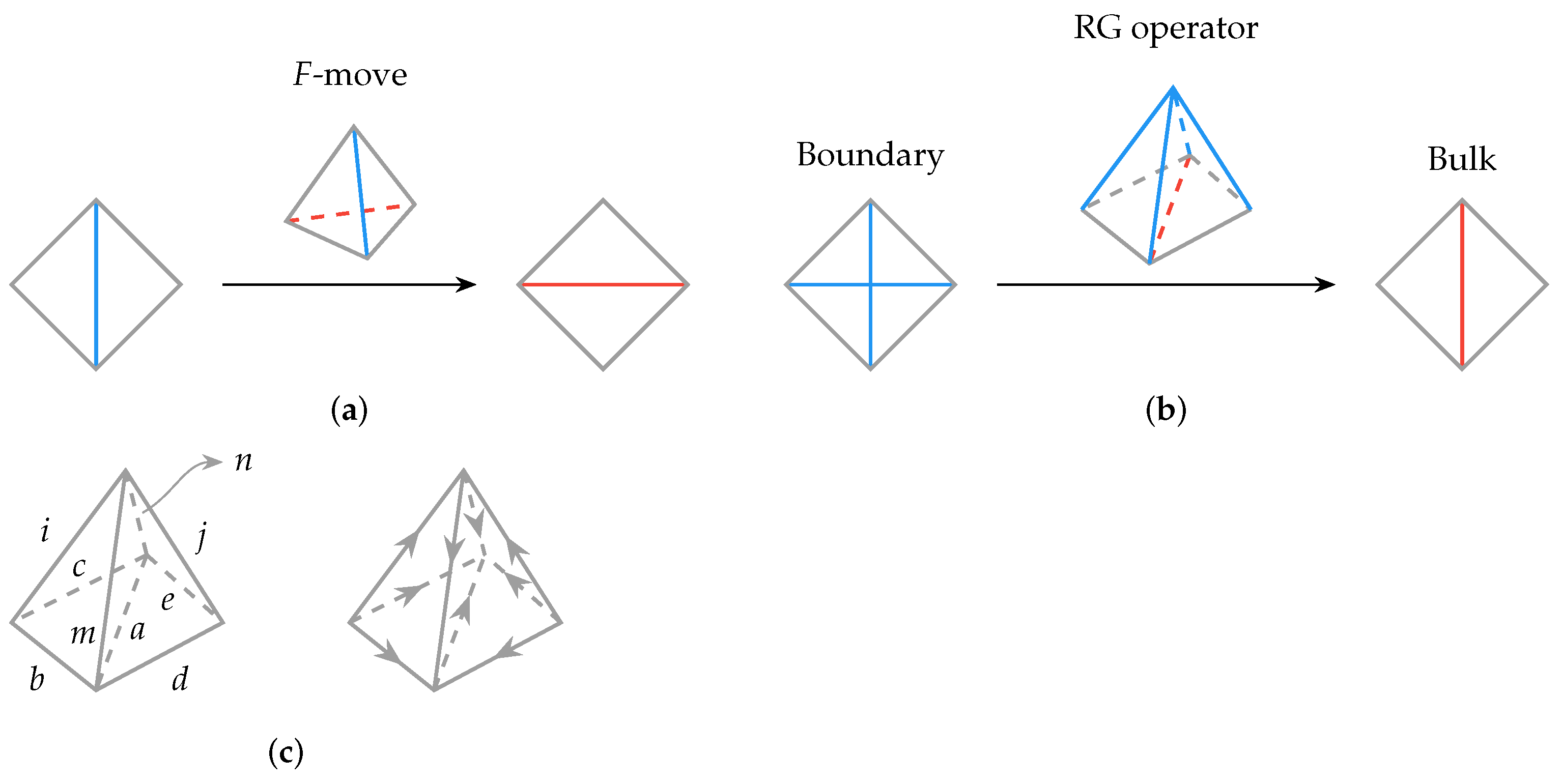
The construction and analysis in the previous section have a natural generalization in one higher dimension. Families of 3D (or 2 + 1D) holographic tensor networks can be constructed from Levin–Wen string net models. The holographic tensor networks constructed from Levin–Wen models were discussed in [18]. The unit tensor constituting the tensor network is represented as a tetrahedron drawn in Figure 3a.
In Figure 3b,c, the RG operator takes edges to a (with as spectators untouched). Therefore, the problem of operator reconstruction can be understood as reconstructing the bulk operator B acting on leg a by operators A acting on legs . We also find the set of operators that are generalized free operators.
Each tetrahedron has six edges which are labeled by the objects in a fusion category characterizing the topological field theory. For a given labeled tetrahedron, the value of an F-symbol is assigned depending on the labels on the six edges. It is non-vanishing if there exists a fusion channel for the three edges of every triangle to fuse to the trivial identity object. Because of this constraint, it is more convenient to think of each allowed configuration of a triangle as our fundamental degrees of freedom (in the bulk) and to consider operators acting on the triangle that transform them between allowed configurations. The problem of operator pushing across the unit tensor can be formulated as pushing the bulk operator action on the triangle basis or .
Since Figure 3c is symmetric, we only need to consider one tetrahedron such as and the other can be simply obtained by flipping all legs. Here, we use the following convention: lowercase letters such as are reserved for edge labels, where n is the number of objects in the fusion category; uppercase are triangle (or face, or fusion channel) labels, and N is the number of admissible configurations on a triangle. The tetrahedron can then be labeled as
![Entropy 25 01543 i003]() where is the triangle label, and function can be determined by fusion rules.
where is the triangle label, and function can be determined by fusion rules.

The constraint equation in 2 + 1D is similar to the 1 + 1D case Equations (8) and (12):
where labels the generalized Pauli matrices in the triangle basis. Now, M is determined by
where is the F-symbol and is quantum dimension of object i in the fusion category.
Similarly, to check whether A can be written in a “simple” form, we look for A of the form, say,
such that
The condition for simple form reconstruction is thus
We can also change it to
to explicitly solve B. Taking indices i, j or i, k to be identical mappings leads to other simple form solutions as well.
3.1. Case
We again look into the simple example where the fusion category is the abelian group . The objects that label the edges of the tetrahedron are again taken from group elements of . We recall that in each admissible triangle, two of the edges must fuse to the third, and fusion here again means a group product of , which was introduced in Equation (24). The number of admissible triangles is thus given by , i.e., the triangles labels lie in . Taking as an example, the admissible triangles (it is also customary to use the dual graph of the triangle to highlight the fusion relation between the edges, which we adopt below) are listed in the following. We also assign a label to each admissible triangle, from 0 to 3.
![Entropy 25 01543 i004]() The above triangle labeling rule for generic n can be stated as
where are two of the edges of the triangle (say, the two top edges when adopting notation as in Equation (45)). We consider the class of trivial Dijkgraaf–Witten models, where all F-symbols equal unity when fusion constraints at each triangle are satisfied (for generic group where the group elements are generically not self-dual, we have to put in an orientation on each edge (see Figure 3c). This can be achieved by numbering the vertices and attaching an arrow to each edge pointing from the vertex with a smaller number to the other with a larger label. The result is independent of such labeling). We have
Therefore, the constraint equation becomes
Now, is a rank- matrix, whose null space is spanned by vectors such that
where , and the specific solution part is
The above triangle labeling rule for generic n can be stated as
where are two of the edges of the triangle (say, the two top edges when adopting notation as in Equation (45)). We consider the class of trivial Dijkgraaf–Witten models, where all F-symbols equal unity when fusion constraints at each triangle are satisfied (for generic group where the group elements are generically not self-dual, we have to put in an orientation on each edge (see Figure 3c). This can be achieved by numbering the vertices and attaching an arrow to each edge pointing from the vertex with a smaller number to the other with a larger label. The result is independent of such labeling). We have
Therefore, the constraint equation becomes
Now, is a rank- matrix, whose null space is spanned by vectors such that
where , and the specific solution part is

For the simple operator case, we check Equation (44), whose coefficients form an matrix with rank , so its null space is spanned by n vectors. In general n, it is difficult to solve Equation (44) and we only consider small n here. For , we have
and
For , the solutions are
and
Here, we use the superscript of to denote its size for clarity.
Other simple form solutions can be calculated in the same way. When , we have
for and
for ; when , we have
for and
for . The corresponding are the same as in Equations (51) and (53).
In Figure 3c, B operators in the two tetrahedra act on triangles and . In the above equations, we see that B can be decomposed into small that act on the edges. For the next iteration of operator pushing, where the bulk is now given by triangles , , and , it can be seen that the A operators acting on edge i and j, as well as the decomposed B operators on edge b, c, d, e, altogether offer the new B operator for these four triangles. Therefore, the operator pushing procedure can be reiterated at the next level.
3.2. Fibonacci Model
Another important example of topological order in the 2 + 1 dimension is the Fibonacci model. As a fusion category, there are two objects 1 and . They satisfy the following fusion rules:
so there are five admissible triangles:
![Entropy 25 01543 i005]() The non-vanishing F symbols are
where denotes the golden ratio. Then,
We can see so the null space of is spanned by three vectors:
The specific solution part for each can thus be calculated; see Supplemental Material.
The non-vanishing F symbols are
where denotes the golden ratio. Then,
We can see so the null space of is spanned by three vectors:
The specific solution part for each can thus be calculated; see Supplemental Material.

For the simple form, we can see the coefficient matrix of Equation (44) is , but it has rank 28, so there is only one solution. However, since the trivial solution ( and B are both identity operators) always exists, there does not exist a non-trivial generalized free field taking the form of
in the Fibonacci model.
We should mention that although not presented here, the above method is in principle applicable to any fusion category such as Ising and models. However, the size of matrix M and grows quickly with the number of objects, so it is difficult to solve the constraint equation for very large systems.
4. Conclusions
In this paper, we explore the emergence of generalized free fields in classes of holographic tensor networks constructed from topological field theories. We consider both 1 + 1D and 2 + 1d networks and demonstrate, for example, in networks following from abelian Dijkgraaf–Witten theories in the trivial cohomological class, the number of generalized free fields scale with the rank of the group. Interestingly, for the simple case of a Fibonacci model in 2 + 1D constructed from the first non-abelian fusion category with the lowest rank, its RG network admits no generalized free field. Of course, to recover a holographic network that resembles a semi-classical bulk theory, it is expected that the spectrum has a large gap with only a sparse number of free fields as the degrees of freedom (i.e., central charge) approaches infinity. While we do not expect such a simple model to admit generalized free fields, it is interesting to find out under what circumstances they would admit some. In the case of RG operators that follow from Dijkgraaf–Witten lattice gauge theories, there are way too many generalized free fields and it is unlikely they are the right candidate for generating a holographic dual with a semi-classical limit. Generic fusion categories however could be plausible.
These models are not expected to recover a semi-classical bulk theory, although they are examples where the dual CFT can be constructed explicitly. It would be interesting to study more generic TQFT with other large “rank” limit to look for bulk networks with semi-classical approximations. These interesting problems are left for future investigations.
Supplementary Materials
The following supporting information can be downloaded at: https://www.mdpi.com/article/10.3390/e25111543/s1.
Author Contributions
Conceptualization, L.-Y.H.; Methodology, X.Z.; Investigation, X.Z.; Writing—original draft, X.Z.; Writing—review & editing, L.-Y.H. All authors have read and agreed to the published version of the manuscript.
Funding
This research was funded by NSFC (Grant No. 11922502, 11875111).
Institutional Review Board Statement
Not applicable.
Data Availability Statement
No new data were created or analyzed in this study. Data sharing is not applicable to this article.
Acknowledgments
The authors thank Xinyang Yu, Yanyan Chen, and Tian Yuan for useful discussions and comments.
Conflicts of Interest
The authors declare no conflict of interest.
References
- Maldacena, J.M. The Large N limit of superconformal field theories and supergravity. Adv. Theor. Math. Phys. 1998, 2, 231–252. [Google Scholar] [CrossRef]
- Witten, E. Anti-de Sitter space and holography. Adv. Theor. Math. Phys. 1998, 2, 253–291. [Google Scholar] [CrossRef]
- Gubser, S.S.; Klebanov, I.R.; Polyakov, A.M. Gauge theory correlators from noncritical string theory. Phys. Lett. B 1998, 428, 105–114. [Google Scholar] [CrossRef]
- Duetsch, M.; Rehren, K.H. Generalized free fields and the AdS-CFT correspondence. Ann. Henri Poincare 2003, 4, 613–635. [Google Scholar] [CrossRef]
- Liu, J.; Perlmutter, E.; Rosenhaus, V.; Simmons-Duffin, D. d-dimensional SYK, AdS Loops, and 6j Symbols. J. High Energy Phys. 2019, 3, 052. [Google Scholar] [CrossRef]
- Collier, S.; Gobeil, Y.; Maxfield, H.; Perlmutter, E. Quantum Regge Trajectories and the Virasoro Analytic Bootstrap. J. High Energy Phys. 2019, 5, 212. [Google Scholar] [CrossRef]
- Nebabu, T.M.; Qi, X. Bulk Reconstruction from Generalized Free Fields. arXiv 2023, arXiv:2306.16687. [Google Scholar]
- Ryu, S.; Takayanagi, T. Holographic derivation of entanglement entropy from AdS/CFT. Phys. Rev. Lett. 2006, 96, 181602. [Google Scholar] [CrossRef] [PubMed]
- Swingle, B. Entanglement Renormalization and Holography. Phys. Rev. D 2012, 86, 065007. [Google Scholar] [CrossRef]
- Pastawski, F.; Yoshida, B.; Harlow, D.; Preskill, J. Holographic quantum error-correcting codes: Toy models for the bulk/boundary correspondence. J. High Energy Phys. 2015, 6, 149. [Google Scholar] [CrossRef]
- Hayden, P.; Nezami, S.; Qi, X.L.; Thomas, N.; Walter, M.; Yang, Z. Holographic duality from random tensor networks. J. High Energy Phys. 2016, 11, 9. [Google Scholar] [CrossRef]
- Bhattacharyya, A.; Gao, Z.S.; Hung, L.Y.; Liu, S.N. Exploring the Tensor Networks/AdS Correspondence. J. High Energy Phys. 2016, 8, 86. [Google Scholar] [CrossRef]
- Bhattacharyya, A.; Hung, L.Y.; Lei, Y.; Li, W. Tensor network and (p-adic) AdS/CFT. J. High Energy Phys. 2018, 1, 139. [Google Scholar] [CrossRef]
- Hamilton, A.; Kabat, D.N.; Lifschytz, G.; Lowe, D.A. Local bulk operators in AdS/CFT: A Boundary view of horizons and locality. Phys. Rev. D 2006, 73, 086003. [Google Scholar] [CrossRef]
- Hamilton, A.; Kabat, D.N.; Lifschytz, G.; Lowe, D.A. Holographic representation of local bulk operators. Phys. Rev. D 2006, 74, 066009. [Google Scholar] [CrossRef]
- Hung, L.Y.; Li, W.; Melby-Thompson, C.M. p-adic CFT is a holographic tensor network. J. High Energy Phys. 2019, 4, 170. [Google Scholar] [CrossRef]
- Vanhove, R.; Bal, M.; Williamson, D.J.; Bultinck, N.; Haegeman, J.; Verstraete, F. Mapping topological to conformal field theories through strange correlators. Phys. Rev. Lett. 2018, 121, 177203. [Google Scholar] [CrossRef] [PubMed]
- Chen, L.; Zhang, H.; Ji, K.; Shen, C.; Wang, R.; Zeng, X.; Hung, L.Y. Exact holographic tensor networks—Constructing CFTD from TQFTD+1. arXiv 2022, arXiv:2210.12127. [Google Scholar]
- Patera, J.; Zassenhaus, H. The Pauli matrices in n dimensions and finest gradings of simple Lie algebras of type An−1. J. Math. Phys. 1988, 29, 665–673. [Google Scholar] [CrossRef]
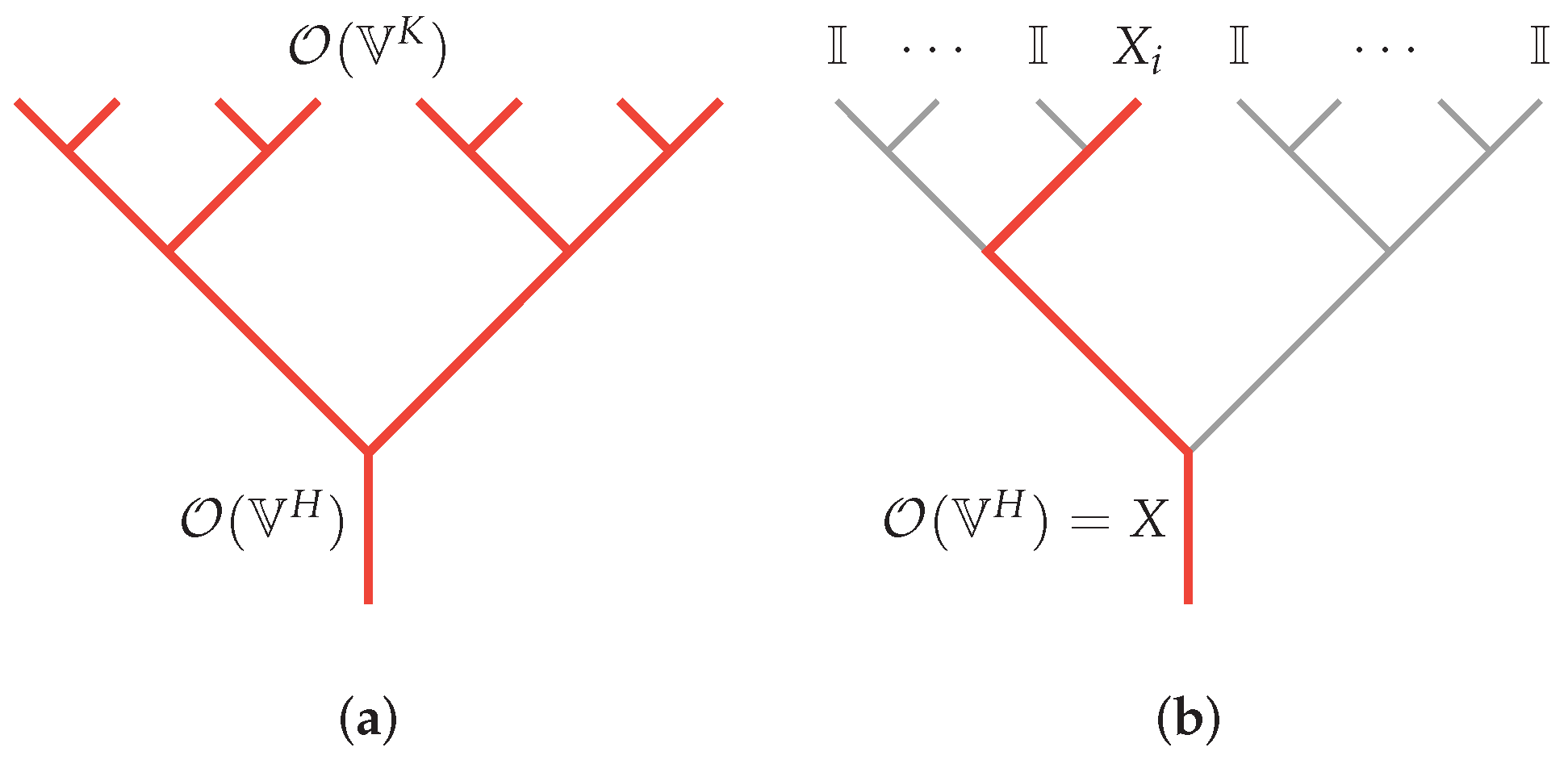
Figure 1.
Operator pushing in a holographic tensor network that is performing coarse-graining. Here, we illustrate a tree-like holographic tensor network. (a) Bulk operator is reconstruced by boundary operator , where we take for simplicity. (b) Bulk operator is reconstruced by a simple form boundary operator as in Equation (3). Hence, it corresponds to a generalized free field.

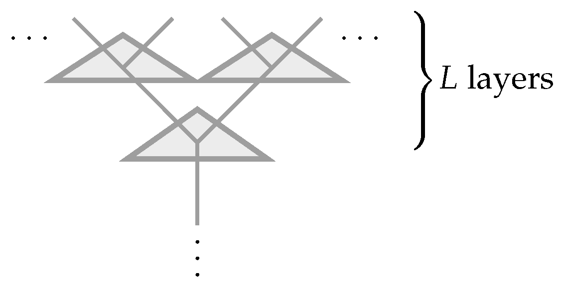
Figure 2.
RG operator in 1 + 1D Dijkgraaf–Witten theory characterized by group G, which takes the form of a tree tensor network with 1D boundary and total number of layers L. The legs are elements of group G. Explicitly, for the untwisted version of Dijkgraaf–Witten theory, each of these three-valent vertices (or dual triangles) resides a tensor . Images from [18] (with modification).

Figure 3.
(a) A single tetrahedron is used as F-move that changes the surface triangulation. It is assigned the value of an F-symbol depending on the labels on the 6 edges. The blue and red lines should be summed over. (b) With two or more tetrahedra, we can construct the RG operator that maps the smaller triangles at the boundary onto larger triangles in the bulk. (c) Arrows on each edge indicate the direction of fusions. If all the objects are self-dual, then these arrows can be ignored.

Disclaimer/Publisher’s Note: The statements, opinions and data contained in all publications are solely those of the individual author(s) and contributor(s) and not of MDPI and/or the editor(s). MDPI and/or the editor(s) disclaim responsibility for any injury to people or property resulting from any ideas, methods, instructions or products referred to in the content. |
© 2023 by the authors. Licensee MDPI, Basel, Switzerland. This article is an open access article distributed under the terms and conditions of the Creative Commons Attribution (CC BY) license (https://creativecommons.org/licenses/by/4.0/).
Share and Cite
MDPI and ACS Style
Zeng, X.; Hung, L.-Y. Bulk Operator Reconstruction in Topological Tensor Network and Generalized Free Fields. Entropy 2023, 25, 1543. https://doi.org/10.3390/e25111543
AMA Style
Zeng X, Hung L-Y. Bulk Operator Reconstruction in Topological Tensor Network and Generalized Free Fields. Entropy. 2023; 25(11):1543. https://doi.org/10.3390/e25111543
Chicago/Turabian StyleZeng, Xiangdong, and Ling-Yan Hung. 2023. "Bulk Operator Reconstruction in Topological Tensor Network and Generalized Free Fields" Entropy 25, no. 11: 1543. https://doi.org/10.3390/e25111543
Note that from the first issue of 2016, this journal uses article numbers instead of page numbers. See further details here.