Nonlinear Fokker–Planck Equations, H-Theorem and Generalized Entropy of a Composed System

Abstract

We investigate the dynamics of a system composed of two different subsystems when subjected to different nonlinear Fokker–Planck equations by considering the H–theorem. We use the H–theorem to obtain the conditions required to establish a suitable dependence for the system’s interaction that agrees with the thermodynamics law when the nonlinearity in these equations is the same. In this framework, we also consider different dynamical aspects of each subsystem and investigate a possible expression for the entropy of the composite system.

1. Introduction

Thermodynamics and statistical mechanics have entropy as a fundamental tool connecting the properties of a system from the particles’ microscopic dynamics with macroscopic quantities and, consequently, with thermodynamic quantities. The concept of entropy started with Clausius’s studies of thermal machines [1]. Subsequently, the Boltzmann and Gibbs works incorporated the concept of probability, building up the fundamentals of statistical mechanics [2,3,4]. It has been successfully applied in many contexts, where the fundamental basis is the molecular chaos hypothesis, which assumes the close-range interaction of molecules and the absence of memory in the collision of particles [5,6]. However, for many physical systems (e.g., fractal and self-organizing structures), conditions for the fulfillment of the molecular chaos hypothesis are not observed as well as the range of the interactions, which are long-ranged [7,8,9]. These points have motivated the analysis of extensions for thermodynamics and statistical physics to cover these scenarios. As an example, Tsallis has proposed an extension of the entropy [10], which has been systematically applied in many contexts such as black holes [11], the electrocaloric effect in quantum dots [12], chemotaxis of biological populations [13], Bose–Einstein condensation [14,15], and stimulated the analysis of other entropies [16,17,18,19,20]. More applications can be found in Refs. [21,22,23,24,25,26]. These entropies verify the H–theorem [27,28,29,30,31], which represents an important result of nonequilibrium statistical mechanics by ensuring that a system will reach an equilibrium after a long time evolution. The H–theorem establishes a connection between the dynamics and entropy, which may be used to investigate the dynamics behind the law of additivity for the different entropies. In this framework, by considering a nonlinear Fokker–Planck equation, the H–theorem can show how the entropy additivity laws can be obtained when a system composed of many subsystems is taken into account. In addition, it can also allow us to obtain the equilibrium distributions.

Here, we investigate through the H–theorem the conditions on the dynamics equations, i.e., nonlinear Fokker–Planck equations [32,33,34,35], for each subsystem of a composed system to reach the equilibrium condition. The results show that generalized entropies imply a coupling between the nonlinear equations. The distributions that emerge from these dynamics equations have a power-law behavior, where each subsystem modifies the other. We also investigate the entropy production for this system. These developments are presented in Section 2. In Section 3, we present our discussions and conclusions.

2. The Problem

Let us start our analysis by establishing the nonlinear Fokker–Planck equations connected to the dynamics of each subsystem of a composed system. They are

$$\begin{array}{c}\hfill \frac{\partial }{\partial t}{\rho }_1(x_1,t)=\Gamma \frac{{\partial }^2}{\partial x_1^2}{P}_1({\rho }_1,t)-\frac{\partial }{\partial x_1}\left[F_1\left(x_1\right){\rho }_1(x_1,t)\right]\end{array}$$

(1)

and

$$\begin{array}{c}\hfill \frac{\partial }{\partial t}{\rho }_2(x_2,t)=\Gamma \frac{{\partial }^2}{\partial x_2^2}{P}_2({\rho }_2,t)-\frac{\partial }{\partial x_2}\left[F_2\left(x_2\right){\rho }_2(x_2,t)\right],\end{array}$$

(2)

where $F_i\left(x_i\right)$, with $i=1$ or 2, represents the external force, i.e., $F_i=-{\partial }_{x_i}{\varphi }_i\left(x_i\right)$ and ${\varphi }_i\left(x_i\right)$ is a potential energy, while $\Gamma$ stands for a generic diffusion coefficient. Notice that $P_1({\rho }_1,t)$ and $P_2({\rho }_2,t)$ present in the diffusive term may have the same form or a different form. Particular choices of $P_i({\rho }_i,t)$ have been successfully analyzed in several problems such as in porous media [36], anomalous diffusion [37], overdamped systems [38], and the Boltzmann equation endowed with a correlation term [39]. In Equations (1) and (2), $P_i({\rho }_i,t)$ will be determined by the H–theorem in connection with the entropic form used to describe the combination of subsystems 1 and 2. It is worth pointing out that the different possibilities may be considered by allowing us to obtain different results for the composite system of 1 and 2 subsystems, as discussed in Refs. [28,29]. However, the combination of these equations, which represent the subsystem 1 and 2, in connection with thermostatistics (e.g., the nonextensive statistics [40]) requires careful analysis with direct consequences on the entropic additivity and zeroth law [41,42,43]. To accomplish this task, we consider general scenarios with different dynamics to investigate possible conditions to Equations (1) and (2) to allow a thermostatistics context.

2.1. H-Theorem

We start our analysis in terms of the H–theorem first by considering $P_1\left({\rho }_1\right)$ and $P_2\left({\rho }_2\right)$ with the same functional form. Afterwards, we consider $P_1\left({\rho }_1\right)$ and $P_2\left({\rho }_2\right)$ with a different functional form. Each one of these cases has different implications for the entropy related to the composed system formed by the systems 1 and 2, with the dynamics given in terms of Equations (1) and (2). Following Refs. [28,29,31], we analyze the behavior of the time derivative of the Helmholtz free energy. This free energy is defined by $F=U-TS$, with the internal energy, U, given by

$$\begin{array}{c}\hfill U={\int }_{-\infty }^{\infty }d{x}_1{\int }_{-\infty }^{\infty }d{x}_2\left[{\varphi }_1\left(x_1\right)+{\varphi }_2\left(x_2\right)\right]{\rho }_1(x_1,t){\rho }_2(x_2,t)\end{array}$$

(3)

and the entropy, S, expressed in terms of an arbitrary function

$$\begin{array}{c}\hfill \mathcal{S}=k{\int }_{-\infty }^{\infty }d{x}_1{\int }_{-\infty }^{\infty }d{x}_{2}s({\rho }_1,{\rho }_2).\end{array}$$

(4)

Note that Equations (3) and (4) represent the total internal energy and the entropy of the system composed of two subsystems governed by Equations (1) and (2), respectively.

By using the previous equations, the total free energy of the system is given by

$$\begin{array}{c}\hfill F={\int }_{-\infty }^{\infty }{\int }_{-\infty }^{\infty }d{x}_{1}d{x}_2\left[\Psi (x_1,x_2){\rho }_1(x_1,t){\rho }_2(x_2,t)-kTs({\rho }_1,{\rho }_2)\right],\end{array}$$

(5)

with $\Psi (x_1,x_2)={\varphi }_1\left(x_1\right)+{\varphi }_2\left(x_2\right)$. Before determining the time derivative of Equation (5), we assume that $P_1({\rho }_1,t)$ and $P_2({\rho }_2,t)$ have essentially the same functional forms and the entropy is a function of the product of the probability densities related to each subsystem, i.e., $s({\rho }_1,{\rho }_2)=s\left({\rho }_1{\rho }_2\right)$. It is then possible to show that

$$\begin{array}{c}\hfill \frac{d}{dt}F={\int }_{-\infty }^{\infty }{\int }_{-\infty }^{\infty }d{x}_{1}d{x}_2\left[\Psi (x_1,x_2)-kT\frac{\partial }{\partial {\rho }_{12}}s\left({\rho }_{12}\right)\right]\frac{\partial }{\partial t}\left[{\rho }_1(x_1,t){\rho }_2(x_2,t)\right],\end{array}$$

(6)

where ${\rho }_{12}={\rho }_1{\rho }_2$, and

$$\begin{array}{ccc}\hfill \frac{d}{dt}F& =& {\int }_{-\infty }^{\infty }{\int }_{-\infty }^{\infty }d{x}_{1}d{x}_2\left\{\Psi (x_1,x_2){\rho }_2-kT{\rho }_2\frac{\partial }{\partial {\rho }_{12}}s\left({\rho }_{12}\right)\right\}\hfill \\ & \times & \frac{\partial }{\partial x_1}\left\{\Gamma \frac{\partial }{\partial x_1}{P}_1({\rho }_1,t)-F_1\left(x_1\right){\rho }_1(x_1,t)\right\}\hfill \\ & +& {\int }_{-\infty }^{\infty }{\int }_{-\infty }^{\infty }d{x}_{1}d{x}_2\left\{\Psi (x_1,x_2){\rho }_1-kT{\rho }_1\frac{\partial }{\partial {\rho }_{12}}s\left({\rho }_{12}\right)\right\}\hfill \\ & \times & \frac{\partial }{\partial x_2}\left\{\Gamma \frac{\partial }{\partial x_2}{P}_2({\rho }_2,t)-F_2\left(x_2\right){\rho }_2(x_2,t)\right\}.\hfill \end{array}$$

(7)

After integration by parts and applying the conditions ${\rho }_i(x\to \pm \infty ,t)\to 0$ and ${\partial }_x{\rho }_i(x\to \pm \infty ,t)\to 0$, we obtain

$$\begin{array}{ccc}\hfill \frac{d}{dt}F& =& -{\int }_{-\infty }^{\infty }{\int }_{-\infty }^{\infty }d{x}_{1}d{x}_2\left\{\frac{\partial }{\partial x_1}{\varphi }_1\left(x_1\right){\rho }_2-kT{\rho }_2^2\frac{\partial {\rho }_1}{\partial x_1}\frac{{\partial }^2}{\partial {\rho }_{12}^2}s\left({\rho }_{12}\right)\right\}\hfill \\ & \times & \left\{\Gamma \frac{\partial }{\partial x_1}{P}_1({\rho }_1,t)-F_1\left(x_1\right){\rho }_1(x_1,t)\right\}\hfill \\ & -& {\int }_{-\infty }^{\infty }{\int }_{-\infty }^{\infty }d{x}_{1}d{x}_2\left\{\frac{\partial }{\partial x_2}{\varphi }_2\left(x_2\right){\rho }_1-kT{\rho }_1^2\frac{\partial {\rho }_2}{\partial x_2}\frac{{\partial }^2}{\partial {\rho }_{12}^2}s\left({\rho }_{12}\right)\right\}\hfill \\ & \times & \left\{\Gamma \frac{\partial }{\partial x_2}{P}_2({\rho }_2,t)-F_2\left(x_2\right){\rho }_2(x_2,t)\right\}.\hfill \end{array}$$

(8)

Now, let us focus on the term

$$\begin{array}{c}\hfill \Gamma \frac{\partial }{\partial x_i}{P}_i({\rho }_i,t)-F_i\left(x_i\right){\rho }_i(x_i,t),\end{array}$$

(9)

where $i=1,2$, which will be directly connected with the properties of the entropy of the composite system. To proceed, we consider that

$$\begin{array}{c}\hfill P_i({\rho }_i,t)={\mathcal{D}}_{j,\gamma }\left(t\right){\rho }_i^{\gamma }(x_i,t)+{\mathcal{D}}_{j,\nu }\left(t\right){\rho }_i^{\nu }(x_i,t),\end{array}$$

(10)

with $j\ne i$, $j=1,2$, and

$$\begin{array}{c}\hfill {\mathcal{D}}_{j,\gamma }\left(t\right)={\alpha }_{\gamma }{\int }_{-\infty }^{\infty }d{x}_j{\rho }_j^{\gamma }(x_j,t)\mathrm{and}{\mathcal{D}}_{j,\nu }\left(t\right)={\alpha }_{\nu }{\int }_{-\infty }^{\infty }d{x}_j{\rho }_j^{\nu }(x_j,t),\end{array}$$

(11)

to be able to cover different scenarios, where ${\alpha }_{\gamma }$ and ${\alpha }_{\nu }$ are constants. Note that the choice of the ${\mathcal{D}}_{j,\gamma }\left(t\right)$ and ${\mathcal{D}}_{j,\nu }\left(t\right)$ implies that each subsystem influences the other. This aspect of the problem can be associated to the feature that the nonlinearity present in Equations (1) and (2) introduces additional interactions between the subsystems during the thermalization process, where each subsystem works as an additional thermal bath to the other. By using the previous equations, we have

$$\begin{array}{ccc}\hfill \frac{d}{dt}F& =& -{\int }_{-\infty }^{\infty }d{x}_1\frac{1}{{\rho }_1}\left\{{\int }_{-\infty }^{\infty }d{x}_2\left[\frac{\partial }{\partial x_1}{\varphi }_1\left(x_1\right){\rho }_2{\rho }_1-kT{\rho }_2^2{\rho }_1\frac{\partial {\rho }_1}{\partial x_1}\frac{{\partial }^2}{\partial {\rho }_{12}^2}s\left({\rho }_{12}\right)\right]\right.\hfill \\ & \times & \left.{\int }_{-\infty }^{\infty }d{x}_2\left[\frac{\partial }{\partial x_1}{\varphi }_1\left(x_1\right){\rho }_1{\rho }_2+\Gamma \frac{\partial {\rho }_1}{\partial x_1}{\rho }_2\frac{\partial }{\partial {\rho }_{12}}\left({\alpha }_{\gamma }{\rho }_2^{\gamma }{\rho }_1^{\gamma }+{\alpha }_{\nu }{\rho }_2^{\nu }{\rho }_1^{\nu }\right)\right]\right\}\hfill \\ & -& {\int }_{-\infty }^{\infty }d{x}_2\frac{1}{{\rho }_2}\left\{{\int }_{-\infty }^{\infty }d{x}_1\left[\frac{\partial }{\partial x_2}{\varphi }_2\left(x_2\right){\rho }_1{\rho }_2-kT{\rho }_1^2{\rho }_2\frac{\partial {\rho }_2}{\partial x_2}\frac{{\partial }^2}{\partial {\rho }_{12}^2}s\left({\rho }_{12}\right)\right]\right.\hfill \\ & \times & {\int }_{-\infty }^{\infty }d{x}_1\left.\left[\frac{\partial }{\partial x_2}{\varphi }_2\left(x_2\right){\rho }_1{\rho }_2+\Gamma \frac{\partial {\rho }_2}{\partial x_2}{\rho }_1\frac{\partial }{\partial {\rho }_{12}}\left({\alpha }_{\gamma }{\rho }_2^{\gamma }{\rho }_1^{\gamma }+{\alpha }_{\nu }{\rho }_2^{\nu }{\rho }_1^{\nu }\right)\right]\right\}.\hfill \end{array}$$

(12)

We verify that

$$\begin{array}{ccc}\hfill \frac{d}{dt}F\le 0\mathrm{for}-kT{\rho }_{12}\frac{{\partial }^2}{\partial {\rho }_{12}^2}s\left({\rho }_{12}\right)& =& \Gamma \frac{\partial }{\partial {\rho }_{12}}\left({\alpha }_{\gamma }{\rho }_2^{\gamma }{\rho }_1^{\gamma }+{\alpha }_{\nu }{\rho }_2^{\nu }{\rho }_1^{\nu }\right)\hfill \\ & =& \Gamma \frac{\partial }{\partial {\rho }_{12}}\left({\alpha }_{\gamma }{\rho }_{12}^{\gamma }+{\alpha }_{\nu }{\rho }_{12}^{\nu }\right),\hfill \end{array}$$

(13)

which implies

$$\begin{array}{ccc}\hfill \frac{d}{dt}F& =& -{\int }_{-\infty }^{\infty }d{x}_1\frac{1}{{\rho }_1}{\left\{{\int }_{-\infty }^{\infty }d{x}_2\left[\frac{\partial }{\partial x_1}{\varphi }_1\left(x_1\right){\rho }_2{\rho }_1-kT{\rho }_2^2{\rho }_1\frac{\partial {\rho }_1}{\partial x_1}\frac{{\partial }^2}{\partial {\rho }_{12}^2}s\left({\rho }_{12}\right)\right]\right\}}^2\hfill \\ & -& {\int }_{-\infty }^{\infty }d{x}_2\frac{1}{{\rho }_2}{\left\{{\int }_{-\infty }^{\infty }d{x}_1\left[\frac{\partial }{\partial x_2}{\varphi }_2\left(x_2\right){\rho }_1{\rho }_2-kT{\rho }_1^2{\rho }_2\frac{\partial {\rho }_2}{\partial x_2}\frac{{\partial }^2}{\partial {\rho }_{12}^2}s\left({\rho }_{12}\right)\right]\right\}}^2.\hfill \end{array}$$

(14)

Consequently, by solving Equation (13) with $\Gamma =kT$ under the conditions defined in Refs. [28,29,30,31], we obtain

$$\begin{array}{c}\hfill s\left({\rho }_{12}\right)=\frac{{\alpha }_{\gamma }}{\gamma -1}\left({\rho }_{12}-{\rho }_{12}^{\gamma }\right)+\frac{{\alpha }_{\nu }}{\nu -1}\left({\rho }_{12}-{\rho }_{12}^{\nu }\right).\end{array}$$

(15)

The entropy for the composite system is given by

$$\begin{array}{ccc}\hfill \mathcal{S}& =& \frac{{\alpha }_{\gamma }k}{\gamma -1}{\int }_{-\infty }^{\infty }d{x}_1{\int }_{-\infty }^{\infty }d{x}_2\left({\rho }_{12}-{\rho }_{12}^{\gamma }\right)\hfill \\ & +& \frac{{\alpha }_{\nu }k}{\nu -1}{\int }_{-\infty }^{\infty }d{x}_1{\int }_{-\infty }^{\infty }d{x}_2\left({\rho }_{12}-{\rho }_{12}^{\nu }\right),\hfill \end{array}$$

(16)

which can also be rewritten as

$$\begin{array}{ccc}\hfill \mathcal{S}& =& \frac{{\alpha }_{\gamma }k}{\gamma -1}{\int }_{-\infty }^{\infty }d{x}_1{\int }_{-\infty }^{\infty }d{x}_2\left[{\rho }_1{\rho }_2-{\left({\rho }_1{\rho }_2\right)}^{\gamma }\right]\hfill \\ & +& \frac{{\alpha }_{\nu }k}{\nu -1}{\int }_{-\infty }^{\infty }d{x}_1{\int }_{-\infty }^{\infty }d{x}_2\left[{\rho }_1{\rho }_2-{\left({\rho }_1{\rho }_2\right)}^{\nu }\right]\hfill \end{array}$$

(17)

and, consequently, as

$$\begin{array}{ccc}\hfill \mathcal{S}& =& \frac{{\alpha }_{\gamma }k}{\gamma -1}\left[1-{\int }_{-\infty }^{\infty }d{x}_1{\int }_{-\infty }^{\infty }d{x}_2{\left({\rho }_1{\rho }_2\right)}^{\gamma }\right]\hfill \\ & +& \frac{{\alpha }_{\nu }k}{\nu -1}\left[1-{\int }_{-\infty }^{\infty }d{x}_1{\int }_{-\infty }^{\infty }d{x}_2{\left({\rho }_1{\rho }_2\right)}^{\nu }\right].\hfill \end{array}$$

(18)

Equation (18) has several particular cases, such as the Tsallis and Kaniadakis entropies, depending on the values of the parameters ${\alpha }_{\gamma }$, ${\alpha }_{\nu }$, $\gamma$, and $\nu$. It is noteworthy that this result preserves the additivity in the Penrose sense [3], i.e., $S\left({\rho }_{12}\right)=S\left({\rho }_1{\rho }_2\right)$ required for a system composed of independent subsystems when the standard entropy is employed.

In the previous context, Equations (1) and (2) can be written as follows:

$$\begin{array}{c}\hfill \frac{\partial }{\partial t}{\rho }_1(x_1,t)={\overline{\mathcal{D}}}_{2,\gamma }\left(t\right)\frac{{\partial }^2}{\partial x_1^2}{\rho }_1^{\gamma }(x_1,t)+{\overline{\mathcal{D}}}_{2,\nu }\left(t\right)\frac{\partial }{\partial x_1^2}{\rho }_1^{\nu }(x_1,t)-\frac{\partial }{\partial x_1}\left[F_1\left(x_1\right){\rho }_1(x_1,t)\right]\end{array}$$

(19)

and

$$\begin{array}{c}\hfill \frac{\partial }{\partial t}{\rho }_2(x_2,t)={\overline{\mathcal{D}}}_{1,\gamma }\left(t\right)\frac{{\partial }^2}{\partial x_2^2}{\rho }_2^{\gamma }(x_2,t)+{\overline{\mathcal{D}}}_{1,\nu }\left(t\right)\frac{{\partial }^2}{\partial x_2^2}{\rho }_2^{\nu }(x_2,t)-\frac{\partial }{\partial x_2}\left[F_2\left(x_2\right){\rho }_2(x_2,t)\right],\end{array}$$

(20)

with ${\overline{\mathcal{D}}}_{i,\gamma }\left(t\right)={\mathcal{D}}_{i,\gamma }\left(t\right)\Gamma$ and ${\overline{\mathcal{D}}}_{i,\nu }\left(t\right)={\mathcal{D}}_{i,\nu }\left(t\right)\Gamma$, by evidencing the influence of one of them on the other. In particular, the terms forming the diffusive part can also be connected with anomalous diffusion processes with different diffusion regimes. The stationary solutions obtained from Equations (19) and (20) are given by

$$\begin{array}{c}\hfill \frac{\gamma }{\gamma -1}{\overline{\mathcal{D}}}_{2,\gamma }{\rho }_{1,st}^{\gamma -1}\left(x_1\right)+\frac{\nu }{\nu -1}{\overline{\mathcal{D}}}_{2,\nu }{\rho }_{1,st}^{\nu -1}\left(x_1\right)={\mathcal{C}}_1-{\varphi }_1\left(x_1\right)\end{array}$$

(21)

and

$$\begin{array}{c}\hfill \frac{\gamma }{\gamma -1}{\overline{\mathcal{D}}}_{1,\gamma }{\rho }_{2,st}^{\gamma -1}\left(x_2\right)+\frac{\nu }{\nu -1}{\overline{\mathcal{D}}}_{1,\nu }{\rho }_{2,st}^{\nu -1}\left(x_2\right)={\mathcal{C}}_2-{\varphi }_2\left(x_2\right),\end{array}$$

(22)

where ${lim}_{t\to \infty }{\overline{\mathcal{D}}}_{i,\gamma }\left(t\right)={\overline{\mathcal{D}}}_{i,\gamma }=\mathrm{constant}$, ${\varphi }_i\left(x\right)$ are potentials with a minimum, and ${\mathcal{C}}_i$ are constants. For the Tsallis entropy, by taking, for simplicity, ${\overline{\mathcal{D}}}_{i,\nu }=0$, we have

$$\begin{array}{c}\hfill {\rho }_{1,st}\left(x_1\right)=\frac{1}{{\mathcal{Z}}_1}{\left[1-(\gamma -1)\frac{{\mathcal{Z}}_1^{\gamma -1}}{\gamma {\overline{\mathcal{D}}}_{2,\gamma }}{\varphi }_1\left(x_1\right)\right]}^{\frac{1}{\gamma -1}}=\frac{1}{{\mathcal{Z}}_1}{exp}_{\gamma }\left[-\frac{{\mathcal{Z}}_1^{\gamma -1}}{\gamma {\overline{\mathcal{D}}}_{2,\gamma }}{\varphi }_1\left(x_1\right)\right]\end{array}$$

(23)

and

$$\begin{array}{c}\hfill {\rho }_{2,st}\left(x_2\right)=\frac{1}{{\mathcal{Z}}_2}{\left[1-(\gamma -1)\frac{{\mathcal{Z}}_2^{\gamma -1}}{\gamma {\overline{\mathcal{D}}}_{2,\gamma }}{\varphi }_1\left(x_2\right)\right]}^{\frac{1}{\gamma -1}}=\frac{1}{{\mathcal{Z}}_2}{exp}_{\gamma }\left[-\frac{{\mathcal{Z}}_2^{\gamma -1}}{\gamma {\overline{\mathcal{D}}}_{1,\gamma }}{\varphi }_2\left(x_2\right)\right],\end{array}$$

(24)

where ${\mathcal{Z}}_i=1/{\left\{[(\gamma -1)/\left(\gamma {\overline{\mathcal{D}}}_{i,\gamma }\right)]{\mathcal{C}}_i\right\}}^{\frac{1}{\gamma -1}}$ is defined by the normalization condition and ${\overline{\mathcal{D}}}_{i,\gamma }=kT{\int }_{-\infty }^{\infty }d{x}_i{\rho }_{i,st}^{\gamma }\left(x_i\right)$. In the preceding equations, ${exp}_q\left[x\right]$ is the $q-$exponential function, defined as follows [40]:

$$\begin{array}{c}\hfill {exp}_q\left[x\right]\equiv \left\{\begin{array}{cc}{(1+(q-1)x)}^{1/(q-1)}& ,x>1/(1-q),\\ 0& ,x<1/(1-q).\end{array}\right.\end{array}$$

(25)

The presence of this function in the previous equations enables the identification of either a short- or a long-tailed behavior of the solution, depending on the value of the parameters $\gamma$ and $\nu$. Indeed, they may have a compact behavior for $\gamma >1$ (or $\nu >1$) due to the cut-off required by the q-exponential to retain the probabilistic interpretation of the distribution. On the other hand, for $\gamma <1$ (or $\nu >1$), the solutions may have the asymptotic limit governed by a power-law behavior, which may also be related to a Lévy distribution [44] and, consequently, asymptotically with the solutions of the fractional Fokker–Planck equations [45], which are asymptotically governed by power-laws.

From the stochastic point of view, Equations (19) and (20) are connected with the following Langevin equations:

$$\begin{array}{c}\hfill {\dot{x}}_1=F_1\left(x_1\right)+\sqrt{2\Gamma {\Lambda }_{1,2}\left(t\right)}{\xi }_1\left(t\right)\end{array}$$

(26)

and

$$\begin{array}{c}\hfill {\dot{x}}_2=F_2\left(x_2\right)+\sqrt{2\Gamma {\Lambda }_{2,1}\left(t\right)}{\xi }_2\left(t\right),\end{array}$$

(27)

where ${\xi }_1\left(t\right)$ and ${\xi }_2\left(t\right)$ are connected to the stochastic forces and ${\Lambda }_{i,j}\left(t\right)={\mathcal{D}}_{j\left(i\right),\gamma \left(\nu \right)}\left(t\right)$${\rho }_{i\left(j\right)}^{\gamma \left(\nu \right)}(x,t)$+${\mathcal{D}}_{j\left(i\right),\nu \left(\gamma \right)}\left(t\right)$${\rho }_{i\left(j\right)}^{\nu \left(\gamma \right)}(x,t)$. In particular, we have

$$\begin{array}{c}\hfill \langle {\xi }_1\rangle =\langle {\xi }_2\rangle =0,\langle {\xi }_1{\xi }_2\rangle =\langle {\xi }_2{\xi }_1\rangle =0\end{array}$$

(28)

and

$$\begin{array}{c}\hfill \langle {\xi }_1\left(t\right){\xi }_1\left(t^{\prime }\right)\rangle \propto \delta (t-t^{\prime }),\langle {\xi }_2\left(t\right){\xi }_2\left(t^{\prime }\right)\rangle \propto \delta (t-t^{\prime }).\end{array}$$

(29)

The walkers related to this problem can be described, for simplicity, in the absence of external forces, in terms of the following equations [46,47]:

$$\begin{array}{c}\hfill {\rho }_1(x_1,t+\tau )={\int }_{-\infty }^{\infty }{\Theta }_{1,2}[x_1-x_1^{\prime },t;\rho (x_1-x_1^{\prime },t)]{\rho }_1(x_1-x_1^{\prime },t)\Phi \left(x_1^{\prime }\right)d{x}_1^{\prime }\end{array}$$

(30)

and

$$\begin{array}{c}\hfill {\rho }_2(x_2,t+\tau )={\int }_{-\infty }^{\infty }{\Theta }_{2,1}[x_2-x_2^{\prime },t;\rho (x_2-x_2^{\prime },t)]{\rho }_2(x_2-x_2^{\prime },t)\Phi \left(x_2^{\prime }\right)d{x}_2^{\prime },\end{array}$$

(31)

where

$$\begin{array}{c}\hfill {\Theta }_{i,j}[x_i,t;\rho (x_i,t)]={\alpha }_{\gamma }{\int }_{-\infty }^{\infty }d{x}_j{\rho }_j^{\gamma }(x_j,t){\rho }_i^{\gamma -1}(x_i,t)+{\alpha }_{\nu }{\int }_{-\infty }^{\infty }d{x}_j{\rho }_j^{\nu }(x_j,t){\rho }_i^{\nu -1}(x_i,t).\end{array}$$

(32)

These equations, in the limit $\tau \to 0$ and $x_i^{\prime }\to 0$, yield Equations (1) and (2) in the absence of external forces, respectively.

Let us now consider a general case, i.e., the one in which the diffusion terms have a different nonlinear dependence on the distributions. This means that the systems have different dynamical aspects governed by the nonlinear dependence on the distribution present in the diffusive term. By using the preceding equations and having in mind Equation (5), we may write

$$\begin{array}{ccc}\hfill \frac{d}{dt}F& =& {\int }_{-\infty }^{\infty }{\int }_{-\infty }^{\infty }d{x}_{1}d{x}_2\left\{\Psi (x_1,x_2)\frac{\partial }{\partial t}\left[{\rho }_1(x_1,t){\rho }_2(x_2,t)\right]\right.\hfill \\ & -& \left.kT\left[\frac{\partial }{\partial {\rho }_1}s({\rho }_1,{\rho }_2)\frac{\partial }{\partial t}{\rho }_1(x_1,t)+\frac{\partial }{\partial {\rho }_2}s({\rho }_1,{\rho }_2)\frac{\partial }{\partial t}{\rho }_2(x_2,t)\right]\right\},\hfill \end{array}$$

(33)

which implies

$$\begin{array}{ccc}\hfill \frac{d}{dt}F& =& {\int }_{-\infty }^{\infty }{\int }_{-\infty }^{\infty }d{x}_{1}d{x}_2\left\{\Psi (x_1,x_2){\rho }_2-kT\frac{\partial }{\partial {\rho }_1}s({\rho }_1,{\rho }_2)\right\}\hfill \\ & \times & \frac{\partial }{\partial x_1}\left\{\Gamma \frac{\partial }{\partial x_1}{P}_1({\rho }_1,t)-F_1\left(x_1\right){\rho }_1(x_1,t)\right\}\hfill \\ & +& {\int }_{-\infty }^{\infty }{\int }_{-\infty }^{\infty }d{x}_{1}d{x}_2\left\{\Psi (x_1,x_2){\rho }_1-kT\frac{\partial }{\partial {\rho }_2}s({\rho }_1,{\rho }_2)\right\}\hfill \\ & \times & \frac{\partial }{\partial x_2}\left\{\Gamma \frac{\partial }{\partial x_2}{P}_2({\rho }_2,t)-F_2\left(x_2\right){\rho }_2(x_2,t)\right\}.\hfill \end{array}$$

(34)

After some calculations, it is possible to show that

$$\begin{array}{ccc}\hfill \frac{d}{dt}F& =& -{\int }_{-\infty }^{\infty }d{x}_1\frac{1}{{\rho }_1}{\int }_{-\infty }^{\infty }d{x}_2\left\{\frac{\partial }{\partial x_1}\varphi \left(x_1\right){\rho }_2{\rho }_1-kT\left[{\rho }_1\frac{{\partial }^2}{\partial {\rho }_1^2}s({\rho }_1,{\rho }_2)\right]\frac{\partial }{\partial x_1}{\rho }_1\right\}\hfill \\ & \times & \left\{\left[\Gamma \frac{\partial }{\partial {\rho }_1}{P}_1({\rho }_1,t)\right]\frac{\partial }{\partial x_1}{\rho }_1-F_1\left(x_1\right){\rho }_1\right\}\hfill \\ & -& {\int }_{-\infty }^{\infty }d{x}_1{\int }_{-\infty }^{\infty }d{x}_2\frac{1}{{\rho }_2}\left\{\frac{\partial }{\partial x_2}\varphi \left(x_2\right){\rho }_1{\rho }_2-kT\left[{\rho }_2\frac{{\partial }^2}{\partial {\rho }_2^2}s({\rho }_1,{\rho }_2)\right]\frac{\partial }{\partial x_2}{\rho }_2\right\}\hfill \\ & \times & \frac{\partial }{\partial x_2}\left\{\left[\Gamma \frac{\partial }{\partial {\rho }_2}{P}_2({\rho }_2,t)\right]\frac{\partial }{\partial x_2}{\rho }_2-F_2\left(x_2\right){\rho }_2\right\}.\hfill \end{array}$$

(35)

Let us analyze in particular the previous equation, for example, for the case

$$\begin{array}{c}\hfill P_1({\rho }_1,t)={\mathcal{D}}_{2,\nu }\left(t\right){\rho }_1^{\gamma }(x_1,t)\mathrm{and}{P}_2({\rho }_2,t)={\mathcal{D}}_{1,\gamma }\left(t\right){\rho }_2^{\nu }(x_2,t),\end{array}$$

(36)

with

$$\begin{array}{c}\hfill {\mathcal{D}}_{2,\nu }\left(t\right)=\frac{1}{\nu -1}{\int }_{-\infty }^{\infty }d{x}_2{\rho }_2^{\nu }(x_2,t)\mathrm{and}{\mathcal{D}}_{1,\gamma }\left(t\right)=\frac{1}{\gamma -1}{\int }_{-\infty }^{\infty }d{x}_1{\rho }_1^{\gamma }(x_1,t),\end{array}$$

(37)

which implies different dynamics for each subsystem. We notice that it is possible to take into account different aspects of the dynamics of each subsystem, and every choice has different implications for the total entropy of the composite system. Similar nonlinear Fokker–Planck equations were considered in Ref. [48] from the point of view of analyzing the interaction between the two subsystems. From Equation (37), we deduce that the entropy needs to satisfy the following equations:

$$\begin{array}{c}\hfill -{\rho }_1\frac{{\partial }^2}{\partial {\rho }_1^2}s({\rho }_1,{\rho }_2)=\frac{\gamma }{\nu -1}{\rho }_2^{\nu }{\rho }_1^{\gamma -1}\mathrm{and}-{\rho }_2\frac{{\partial }^2}{\partial {\rho }_2^2}s({\rho }_1,{\rho }_2)=\frac{\nu }{\gamma -1}{\rho }_2^{\nu -1}{\rho }_1^{\gamma }\end{array}$$

(38)

in order to verify

$$\begin{array}{c}\hfill \frac{d}{dt}F\le 0,\end{array}$$

(39)

and, consequently, to satisfy the H–theorem. A solution for the previous system of equations is

$$\begin{array}{c}\hfill s({\rho }_1,{\rho }_2)=\frac{1}{(\nu -1)(\gamma -1)}\left({\rho }_1{\rho }_2-{\rho }_2^{\nu }{\rho }_1^{\gamma }\right).\end{array}$$

(40)

This result allows us to write the total entropy of this system as follows:

$$\begin{array}{c}\hfill \mathcal{S}=\frac{k}{(\nu -1)(\gamma -1)}\left[1-{\int }_{-\infty }^{\infty }d{x}_2{\rho }_2^{\nu }(x_2,t){\int }_{-\infty }^{\infty }d{x}_1{\rho }_1^{\gamma }(x_1,t)\right].\end{array}$$

(41)

It is remarkable that this result for the entropy differs from the preceding one given by Equation (18), obtained from a different choice of nonlinear Fokker–Planck equations. Equation (41) results from a combination of different subsystems with different dynamics, which individually have different entropies associated with them. One of the consequences is that the entropy of the composite system, for this specific case, can not be written as $S\left({\rho }_1{\rho }_2\right)$, only when $\gamma =\nu$. Another remarkable point is the connection of Equation (41) with the composition of Tsallis entropies of different q-indices [49,50]. The solution can be found in this framework using the q-exponential functions. In particular, it is possible to show that the solution for each nonlinear Fokker–Planck equation, in the absence of external force, is

$$\begin{array}{c}\hfill {\rho }_1(x_1,t)={exp}_{\gamma }\left[-{\beta }_1\left(t\right)x_1^2\right]/{\mathcal{Z}}_1\left(t\right)\end{array}$$

(42)

and

$$\begin{array}{c}\hfill {\rho }_2(x_1,t)={exp}_{\nu }\left[-{\beta }_2\left(t\right)x_2^2\right]/{\mathcal{Z}}_2\left(t\right),\end{array}$$

(43)

with ${\beta }_1\left(t\right)$, ${\beta }_2\left(t\right)$, ${\mathcal{Z}}_1\left(t\right)$, and ${\mathcal{Z}}_2\left(t\right)$ obtained from the following set of equations:

$$\begin{array}{ccc}\hfill \frac{1}{2{\beta }_1}\frac{d}{dt}{\beta }_1& =& -\frac{2\gamma }{\nu -1}\frac{{\mathcal{I}}_{\nu }}{{\mathcal{Z}}_2^{\nu }\sqrt{{\beta }_2}}{\beta }_1{\mathcal{Z}}_1^{1-\gamma },-\frac{1}{{\mathcal{Z}}_1}\frac{d}{dt}{\mathcal{Z}}_1=-\frac{2\gamma }{\nu -1}\frac{{\mathcal{I}}_{\nu }}{{\mathcal{Z}}_2^{\nu }\sqrt{{\beta }_2}}{\beta }_1{\mathcal{Z}}_1^{1-\gamma },\hfill \end{array}$$

(44)

$$\begin{array}{ccc}\hfill \frac{1}{2{\beta }_2}\frac{d}{dt}{\beta }_2& =& -\frac{2\nu }{\gamma -1}\frac{{\mathcal{I}}_{\gamma }}{{\mathcal{Z}}_1^{\gamma }\sqrt{{\beta }_1}}{\beta }_2{\mathcal{Z}}_2^{1-\nu },-\frac{1}{{\mathcal{Z}}_2}\frac{d}{dt}{\mathcal{Z}}_2=-\frac{2\nu }{\gamma -1}\frac{{\mathcal{I}}_{\gamma }}{{\mathcal{Z}}_1^{\gamma }\sqrt{{\beta }_1}}{\beta }_2{\mathcal{Z}}_2^{1-\nu },\hfill \end{array}$$

(45)

with

$$\begin{array}{c}\hfill {\mathcal{I}}_{\kappa }=\left\{\begin{array}{cc}\frac{\Gamma \left(\frac{1}{2}\right)\Gamma \left(1+\frac{\kappa }{\kappa -1}\right)}{\sqrt{\kappa -1}\Gamma \left(\frac{3}{2}+\frac{\kappa }{\kappa -1}\right)}& 1\le \kappa <2\\ \frac{\Gamma \left(\frac{1}{2}\right)\Gamma \left(\frac{\kappa }{1-\kappa }-\frac{1}{2}\right)}{\sqrt{1-\kappa }\Gamma \left(\frac{\kappa }{1-\kappa }\right)}& 0\le \kappa \le 1\end{array}\right.,\end{array}$$

(46)

where $\kappa =\gamma$ or $\nu$.

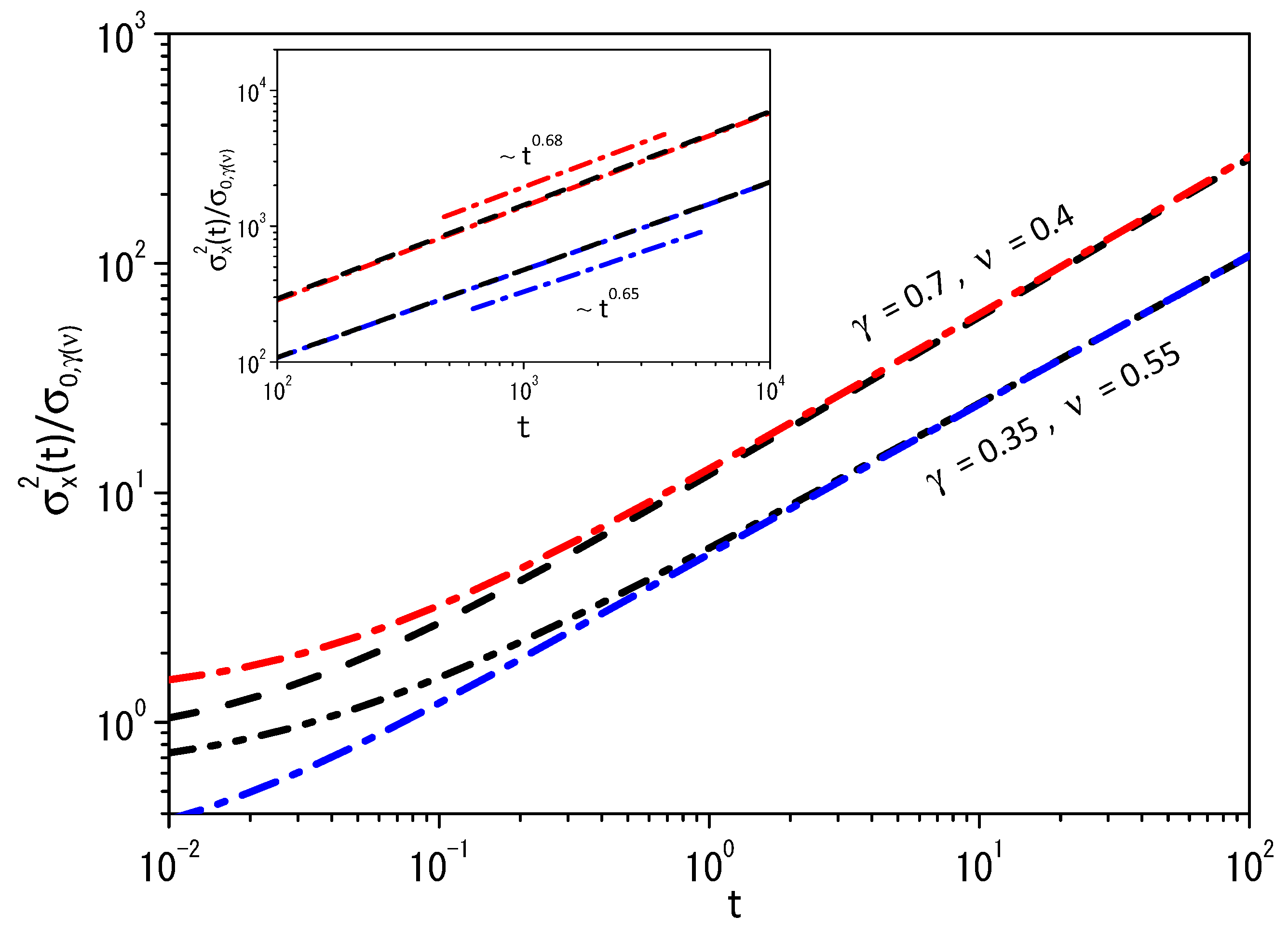
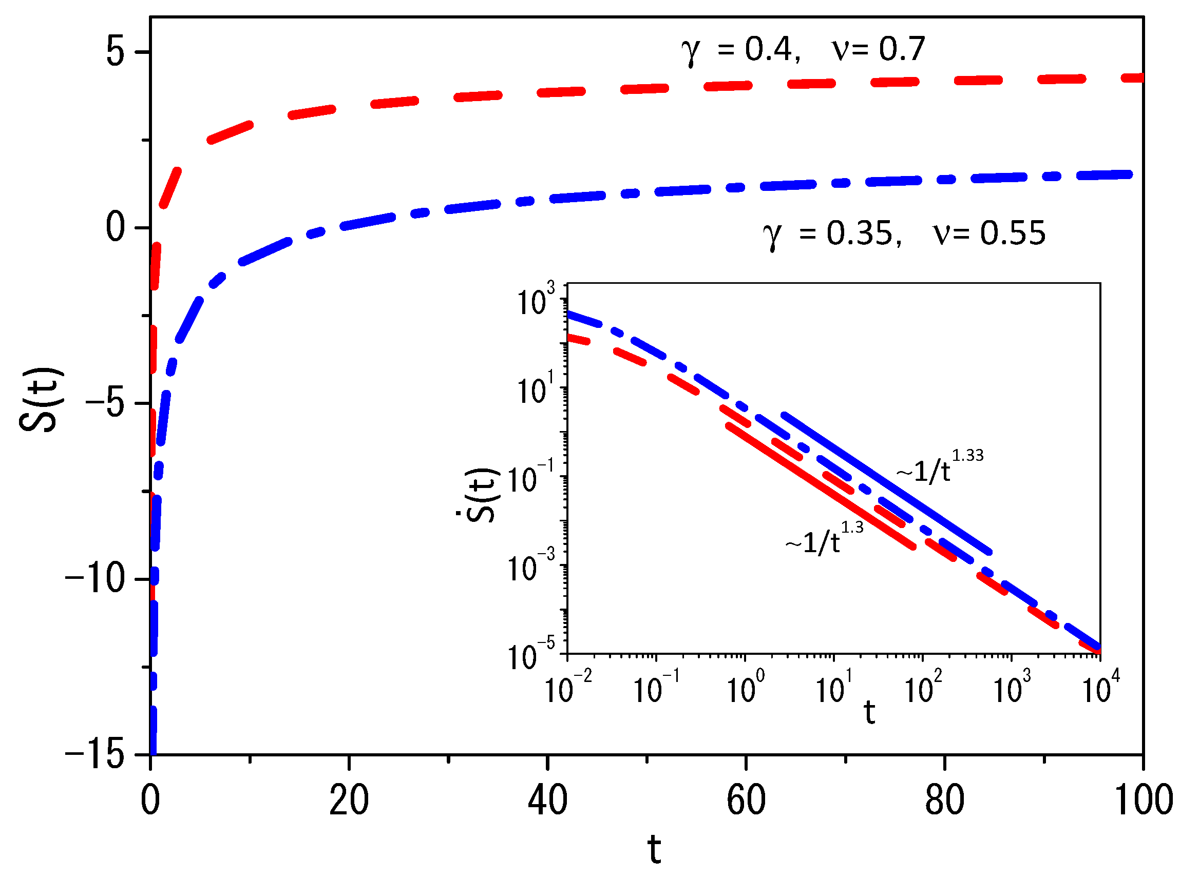
Figure 1 shows the behavior of the mean square displacement for two different sets of $\gamma$ and $\nu$ in the absence of external forces. The values chosen for the parameters $\gamma$ and $\nu$ are responsible for different behaviors of the mean square displacement for each case, as pointed out in the inset of Figure 1. In particular, the diffusion present in this scenario is anomalous [51,52]. Figure 2 shows the behavior of Equation (41) for two different sets of $\gamma$ and $\nu$. Note that different values of ${\beta }_1\left(0\right)$ and ${\beta }_2\left(0\right)$ used to obtain Figure 1 and Figure 2 are connected to different initial conditions for each subsystem. This is the reason why we initially verified different behaviors for each set of the parameters $\gamma$ and $\nu$, and, after some time, the mean square displacement has the same time dependence for both subsystems. The entropy production is shown in the inset in Figure 2, which corresponds to the behavior of Equation (61) for the entropy given by Equation (41). We underline that the system composed of these two systems reaches equilibrium in the limit of $t\to \infty$, since in this limit $\dot{S}\left(t\right)\to 0$. For general nonlinear Fokker–Planck equations, the entropy should simultaneously satisfy the following equations,

$$\begin{array}{c}\hfill -{\rho }_1\frac{{\partial }^2}{\partial {\rho }_1^2}s({\rho }_1,{\rho }_2)=\frac{\partial }{\partial {\rho }_1}{P}_1({\rho }_1,t)\mathrm{and}-{\rho }_2\frac{{\partial }^2}{\partial {\rho }_2^2}s({\rho }_1,{\rho }_2)=\frac{\partial }{\partial {\rho }_2}{P}_2({\rho }_2,t),\end{array}$$

(47)

to verify $\frac{d}{dt}F\le 0$ and, consequently, satisfy the H–theorem. It is also significant to mention that, depending on the form of the nonlinear dependence in the Equations (1) and (2), which may not recover the standard form of the Fokker–Planck equation, the entropy associated with these equations will not recover the usual form.

2.2. Entropy Production

Let us analyze the entropy production related to Equation (17) with the dynamics of ${\rho }_1(x_1,t)$ and ${\rho }_2(x_2,t)$ given by Equations (19) and (20). By performing a time derivative of Equation (17), we obtain

$$\begin{array}{ccc}\hfill \frac{d}{dt}\mathcal{S}\left(t\right)& =& k{\int }_{-\infty }^{\infty }{\int }_{-\infty }^{\infty }d{x}_{1}d{x}_2\left[\frac{\partial }{\partial {\rho }_{12}}s\left({\rho }_{12}\right)\right]\frac{\partial }{\partial t}\left[{\rho }_1(x_1,t){\rho }_2(x_2,t)\right]\hfill \\ & =& -k{\int }_{-\infty }^{\infty }d{x}_1{\int }_{-\infty }^{\infty }d{x}_2{\rho }_2\frac{\partial }{\partial {\rho }_{12}}s\left({\rho }_{12}\right)\frac{\partial }{\partial x_1}{\mathcal{J}}_1(x_1,t)\hfill \\ & -& k{\int }_{-\infty }^{\infty }d{x}_1{\rho }_1{\int }_{-\infty }^{\infty }d{x}_2\frac{\partial }{\partial {\rho }_{12}}s\left({\rho }_{12}\right)\frac{\partial }{\partial x_2}{\mathcal{J}}_2(x_2,t)\hfill \end{array}$$

(48)

and, consequently, performing integration by parts with the conditions ${\mathcal{J}}_1(x_1\to \pm \infty ,t)\to 0$ and ${\mathcal{J}}_2(x_2\to \pm \infty ,t)\to 0$, also

$$\begin{array}{ccc}\hfill \frac{d}{dt}\mathcal{S}\left(t\right)& =& k{\int }_{-\infty }^{\infty }d{x}_1{\int }_{-\infty }^{\infty }d{x}_2\left[{\rho }_2^2\frac{{\partial }^2}{\partial {\rho }_{12}^2}s\left({\rho }_{12}\right)\frac{\partial {\rho }_1}{\partial x_1}\right]{\mathcal{J}}_1(x_1,t)\hfill \\ & +& k{\int }_{-\infty }^{\infty }d{x}_1{\int }_{-\infty }^{\infty }d{x}_2\left[{\rho }_1^2\frac{{\partial }^2}{\partial {\rho }_{12}^2}s\left({\rho }_{12}\right)\frac{\partial {\rho }_2}{\partial x_2}\right]{\mathcal{J}}_2(x_2,t).\hfill \end{array}$$

(49)

It is possible to simplify Equation (48) by using, from the H–theorem, the equations

$$\begin{array}{c}\hfill -kT{\rho }_1{\rho }_2^2\frac{\partial {\rho }_1}{\partial x_1}\frac{{\partial }^2}{\partial {\rho }_{12}^2}s\left({\rho }_{12}\right)=\Gamma \frac{\partial }{\partial x_1}{P}_1({\rho }_1,t)\end{array}$$

(50)

and

$$\begin{array}{c}\hfill -kT{\rho }_2{\rho }_1^2\frac{\partial {\rho }_2}{\partial x_2}\frac{{\partial }^2}{\partial {\rho }_{12}^2}s\left({\rho }_{12}\right)=\Gamma \frac{\partial }{\partial x_2}{P}_2({\rho }_2,t),\end{array}$$

(51)

in order to obtain

$$\begin{array}{ccc}\hfill \frac{d}{dt}\mathcal{S}\left(t\right)& =& -\frac{1}{T}{\int }_{-\infty }^{\infty }d{x}_1{F}_1\left(x_1\right){\mathcal{J}}_1(x_1,t)-\frac{1}{T}{\int }_{-\infty }^{\infty }d{x}_2{F}_2\left(x_2\right){\mathcal{J}}_2(x_2,t)\hfill \\ & +& \frac{1}{T}{\int }_{-\infty }^{\infty }d{x}_1\frac{{\mathcal{J}}_1^2(x_1,t)}{{\rho }_1(x_1,t)}+\frac{1}{T}{\int }_{-\infty }^{\infty }d{x}_2\frac{{\mathcal{J}}_2^2(x_2,t)}{{\rho }_2(x_2,t)},\hfill \end{array}$$

(52)

where

$$\begin{array}{c}\hfill {\mathcal{J}}_1(x_1,t)=-\Gamma \frac{\partial }{\partial x_1}{P}_1({\rho }_1,t)+F_1\left(x_1\right){\rho }_1(x_1,t)\end{array}$$

(53)

and

$$\begin{array}{c}\hfill {\mathcal{J}}_2(x_2,t)=-\Gamma \frac{\partial }{\partial x_2}{P}_2({\rho }_2,t)+F_2\left(x_2\right){\rho }_2(x_2,t),\end{array}$$

(54)

with $P_1({\rho }_1,t)$ and $P_2({\rho }_2,t)$ given by Equations (10) and (11). Equation (48) can be written as follows:

$$\begin{array}{c}\hfill \frac{d}{dt}\mathcal{S}=\Pi -\Phi \end{array}$$

(55)

where one identifies the entropy flux, representing the exchanges of entropy between the subsystems represented by ${\rho }_1$ and ${\rho }_2$ and their neighborhood,

$$\begin{array}{c}\hfill \Phi =\frac{1}{T}{\int }_{-\infty }^{\infty }d{x}_1{F}_1\left(x_1\right){\mathcal{J}}_1(x_1,t)+\frac{1}{T}{\int }_{-\infty }^{\infty }d{x}_2{F}_2\left(x_2\right){\mathcal{J}}_2(x_2,t),\end{array}$$

(56)

as well as the entropy-production contribution:

$$\begin{array}{c}\hfill \Pi =\frac{1}{T}{\int }_{-\infty }^{\infty }d{x}_1\frac{{\mathcal{J}}_1^2(x_1,t)}{{\rho }_1(x_1,t)}+\frac{1}{T}{\int }_{-\infty }^{\infty }d{x}_2\frac{{\mathcal{J}}_2^2(x_2,t)}{{\rho }_2(x_2,t)}.\end{array}$$

(57)

We underline that T and ${\rho }_i(x_i,t)$ are positive quantities, yielding the desirable result: $\Pi \ge 0$.

For the general case represented by Equation (4), we have

$$\begin{array}{ccc}\hfill \frac{d}{dt}\mathcal{S}\left(t\right)& =& k{\int }_{-\infty }^{\infty }{\int }_{-\infty }^{\infty }d{x}_{1}d{x}_2\left[\frac{\partial }{\partial {\rho }_1}s({\rho }_1,{\rho }_2)\frac{\partial }{\partial t}{\rho }_1(x_1,t)+\frac{\partial }{\partial {\rho }_2}s({\rho }_1,{\rho }_2)\frac{\partial }{\partial t}{\rho }_2(x_2,t)\right]\hfill \\ & =& -k{\int }_{-\infty }^{\infty }{\int }_{-\infty }^{\infty }d{x}_{1}d{x}_2\frac{\partial }{\partial {\rho }_1}s({\rho }_1,{\rho }_2)\frac{\partial }{\partial x_1}{\mathcal{J}}_1(x_1,t)\hfill \\ & -& k{\int }_{-\infty }^{\infty }{\int }_{-\infty }^{\infty }d{x}_{1}d{x}_2\frac{\partial }{\partial {\rho }_2}s({\rho }_1,{\rho }_2)\frac{\partial }{\partial x_2}{\mathcal{J}}_2(x_2,t).\hfill \end{array}$$

(58)

Performing integration by parts in Equation (58) and by taking into account the conditions ${\mathcal{J}}_1(x_1\to \pm \infty ,t)\to 0$ and ${\mathcal{J}}_2(x_2\to \pm \infty ,t)\to 0$, we obtain that

$$\begin{array}{ccc}\hfill \frac{d}{dt}\mathcal{S}\left(t\right)& =& k{\int }_{-\infty }^{\infty }{\int }_{-\infty }^{\infty }d{x}_{1}d{x}_2\left[\frac{\partial {\rho }_1}{\partial x_1}\frac{{\partial }^2}{\partial {\rho }_1^2}s({\rho }_1,{\rho }_2)\right]{\mathcal{J}}_1(x_1,t)\hfill \\ & +& k{\int }_{-\infty }^{\infty }{\int }_{-\infty }^{\infty }d{x}_{1}d{x}_2\left[\frac{\partial {\rho }_2}{\partial x_2}\frac{{\partial }^2}{\partial {\rho }_2^2}s({\rho }_1,{\rho }_2)\right]{\mathcal{J}}_2(x_2,t).\hfill \end{array}$$

(59)

By using the equations,

$$\begin{array}{c}\hfill -{\rho }_1\frac{\partial {\rho }_1}{\partial x_1}\frac{{\partial }^2}{\partial {\rho }_1^2}s({\rho }_1,{\rho }_2)=\frac{\partial }{\partial x_1}{P}_1({\rho }_1,t)\mathrm{and}-{\rho }_2\frac{\partial {\rho }_2}{\partial x_2}\frac{{\partial }^2}{\partial {\rho }_2^2}s({\rho }_1,{\rho }_2)=\frac{\partial }{\partial x_2}{P}_2({\rho }_2,t),\end{array}$$

(60)

it is possible to simplify Equation (59) in order to obtain

$$\begin{array}{ccc}\hfill \frac{d}{dt}\mathcal{S}\left(t\right)& =& -\frac{1}{T}{\int }_{-\infty }^{\infty }d{x}_1{F}_1\left(x_1\right){\mathcal{J}}_1(x_1,t)-\frac{1}{T}{\int }_{-\infty }^{\infty }d{x}_2{F}_2\left(x_2\right){\mathcal{J}}_2(x_2,t)\hfill \\ & +& \frac{1}{T}{\int }_{-\infty }^{\infty }d{x}_1\frac{{\mathcal{J}}_1^2(x_1,t)}{{\rho }_1(x_1,t)}+\frac{1}{T}{\int }_{-\infty }^{\infty }d{x}_2\frac{{\mathcal{J}}_2^2(x_2,t)}{{\rho }_2(x_2,t)},\hfill \end{array}$$

(61)

where

$$\begin{array}{c}\hfill {\mathcal{J}}_1(x_1,t)=-\Gamma \frac{\partial }{\partial x_1}{P}_1({\rho }_1,t)+F_1\left(x_1\right){\rho }_1(x_1,t)\end{array}$$

(62)

and

$$\begin{array}{c}\hfill {\mathcal{J}}_2(x_2,t)=-\Gamma \frac{\partial }{\partial x_2}{P}_2({\rho }_2,t)+F_2\left(x_2\right){\rho }_2(x_2,t),\end{array}$$

(63)

as before, with $P_1({\rho }_1,t)$ and $P_2({\rho }_2,t)$ arbitrary. Note that Equation (61) is formally equal to Equation (52), which evidences that the result obtained for the entropy production is invariant in form when the entropies are obtained from the H–theorem.

3. Discussion and Conclusions

We have investigated the entropy of a system composed of two subsystems governed by nonlinear Fokker–Planck equations. In this context, we have essentially analyzed two scenarios; in one of them, the subsystems have the same dynamics, and in the other one, they have different dynamics, i.e., the nonlinear Fokker–Planck equations are different. The first case allows the definition of entropy which can be connected to different cases and preserves the formal structure $S({\rho }_1,{\rho }_2)=S\left({\rho }_1{\rho }_2\right)$ also verified by the standard entropy of Boltzmann–Gibbs. For the other case, we consider different dynamics for each subsystem, which allows the definition of an entropic form for which $S({\rho }_1,{\rho }_2)\ne S\left({\rho }_1{\rho }_2\right)$. In both cases, we have analyzed the entropy production and we have shown the effect of each subsystem on the composite system. In addition, we have shown that the time variation of the entropy (entropy production) for the total system is invariant in form for all the cases considered here.

References

- Clausius, R. The Mechanical Theory of Heat: With Its Appli- cations to the Steam-Engine and to the Physical Properties of Bodies; Macmillan: New York, NY, USA, 1879. [Google Scholar]
- Bryan, G. Elementary principles in statistical mechanics. Nature 1902, 66, 291–292. [Google Scholar] [CrossRef]
- Penrose, O. Foundations of Statistical Mechanics: A Deductive Treatment; Courier Corporation: Washington, DC, USA, 2005. [Google Scholar]
- Sandler, S.I.; Woodcock, L.V. Historical observations on laws of thermodynamics. J. Chem. Eng. Data 2010, 55, 4485–4490. [Google Scholar] [CrossRef]
- Bogoliubov, N.N. Problems of Dynamic Theory in Statistical Physics; Technical Information Service, United States Atomic Energy Commission: Washington, DC, USA, 1960. [Google Scholar]
- Hill, T.L. Statistical Mechanics: Principles and Selected Applications; Courier Corporation: Washington, DC, USA, 2013. [Google Scholar]
- Abe, S.; Okamoto, Y. Nonextensive Statistical Mechanics and Its Applications; Springer Science & Business Media: Berlin/Heidelberg, Germany, 2001; Volume 560. [Google Scholar]
- Mukamel, D. Statistical mechanics of systems with long range interactions. In Proceedings of the AIP Conference Proceedings; American Institute of Physics: Melville, NY, USA, 2008; Volume 970, pp. 22–38. [Google Scholar]
- Singh, R.; Moessner, R.; Roy, D. Effect of long-range hopping and interactions on entanglement dynamics and many-body localization. Phys. Rev. B 2017, 95, 094205. [Google Scholar] [CrossRef]
- Tsallis, C. Possible generalization of Boltzmann-Gibbs statistics. J. Stat. Phys. 1988, 52, 479–487. [Google Scholar] [CrossRef]
- Nojiri, S.; Odintsov, S.D.; Faraoni, V. From nonextensive statistics and black hole entropy to the holographic dark universe. Phys. Rev. D 2022, 105, 044042. [Google Scholar] [CrossRef]
- Khordad, R.; Sedehi, H. Electrocaloric effect in quantum dots using the non-extensive formalism. Opt. Quantum Electron. 2022, 54, 511. [Google Scholar] [CrossRef]
- Chavanis, P.H. Nonlinear mean field Fokker-Planck equations. Application to the chemotaxis of biological populations. Eur. Phys. J. B 2008, 62, 179–208. [Google Scholar] [CrossRef]
- Megías, E.; Timóteo, V.; Gammal, A.; Deppman, A. Bose–Einstein condensation and non-extensive statistics for finite systems. Phys. A Stat. Mech. Its Appl. 2022, 585, 126440. [Google Scholar] [CrossRef]
- Rajagopal, A.; Mendes, R.; Lenzi, E. Quantum statistical mechanics for nonextensive systems: Prediction for possible experimental tests. Phys. Rev. Lett. 1998, 80, 3907. [Google Scholar] [CrossRef]
- Lenzi, E.; Mendes, R.; Da Silva, L. Statistical mechanics based on Renyi entropy. Phys. A Stat. Mech. Its Appl. 2000, 280, 337–345. [Google Scholar] [CrossRef]
- Lopes, A.M.; Machado, J.A.T. A review of fractional order entropies. Entropy 2020, 22, 1374. [Google Scholar] [CrossRef] [PubMed]
- Lenzi, E.; Scarfone, A. Extensive-like and intensive-like thermodynamical variables in generalized thermostatistics. Phys. A Stat. Mech. Its Appl. 2012, 391, 2543–2555. [Google Scholar] [CrossRef]
- da Silva, J.; da Silva, G.; Ramos, R. The Lambert-Kaniadakis Wκ function. Phys. Lett. A 2020, 384, 126175. [Google Scholar] [CrossRef]
- Kaniadakis, G. Maximum entropy principle and power-law tailed distributions. Eur. Phys. J. B 2009, 70, 3–13. [Google Scholar] [CrossRef]
- Oylukan, A.D.; Shizgal, B. Nonequilibrium distributions from the Fokker-Planck equation: Kappa distributions and Tsallis entropy. Phys. Rev. E 2023, 108, 014111. [Google Scholar] [CrossRef] [PubMed]
- Lutz, E. Anomalous diffusion and Tsallis statistics in an optical lattice. Phys. Rev. A 2003, 67, 051402. [Google Scholar] [CrossRef]
- Borland, L. Ito-Langevin equations within generalized thermostatistics. Phys. Lett. A 1998, 245, 67–72. [Google Scholar] [CrossRef]
- Chavanis, P.H. Generalized Euler, Smoluchowski and Schrödinger equations admitting self-similar solutions with a Tsallis invariant profile. Eur. Phys. J. Plus 2019, 134, 353. [Google Scholar] [CrossRef]
- Kaniadakis, G.; Lapenta, G. Microscopic dynamics underlying anomalous diffusion. Phys. Rev. E 2000, 62, 3246–3249. [Google Scholar] [CrossRef]
- Frank, T. A Langevin approach for the microscopic dynamics of nonlinear Fokker–Planck equations. Phys. A Stat. Mech. Its Appl. 2001, 301, 52–62. [Google Scholar] [CrossRef]
- Kaniadakis, G. H–theorem and generalized entropies within the framework of nonlinear kinetics. Phys. Lett. A 2001, 288, 283–291. [Google Scholar] [CrossRef]
- Plastino, A.; Wedemann, R.; Nobre, F. H–theorems for systems of coupled nonlinear Fokker-Planck equations. Europhys. Lett. 2022, 139, 11002. [Google Scholar] [CrossRef]
- Dos Santos, M.; Lenzi, E. Entropic nonadditivity, H theorem, and nonlinear Klein-Kramers equations. Phys. Rev. E 2017, 96, 052109. [Google Scholar] [CrossRef]
- dos Santos, M.; Lenzi, M.; Lenzi, E. Nonlinear Fokker–Planck equations, H–theorem, and entropies. Chin. J. Phys. 2017, 55, 1294–1299. [Google Scholar] [CrossRef]
- Casas, G.; Nobre, F.; Curado, E. Entropy production and nonlinear Fokker-Planck equations. Phys. Rev. E 2012, 86, 061136. [Google Scholar] [CrossRef] [PubMed]
- Frank, T.D. Nonlinear Fokker-Planck Equations: Fundamentals and Applications; Springer Science & Business Media: Berlin/Heidelberg, Germany, 2005. [Google Scholar]
- Schwämmle, V.; Nobre, F.D.; Curado, E.M. Consequences of the H theorem from nonlinear Fokker-Planck equations. Phys. Rev. E 2007, 76, 041123. [Google Scholar] [CrossRef] [PubMed]
- Schwämmle, V.; Curado, E.M.; Nobre, F.D. A general nonlinear Fokker-Planck equation and its associated entropy. Eur. Phys. J. B 2007, 58, 159–165. [Google Scholar] [CrossRef]
- Pedron, I.T.; Mendes, R.; Malacarne, L.C.; Lenzi, E.K. Nonlinear anomalous diffusion equation and fractal dimension: Exact generalized Gaussian solution. Phys. Rev. E 2002, 65, 041108. [Google Scholar] [CrossRef]
- Vázquez, J.L. The Porous Medium Equation: Mathematical Theory; Oxford University Press: Oxford, UK, 2007. [Google Scholar]
- Casas, G.A.; Nobre, F.D. Nonlinear Fokker-Planck equations in super-diffusive and sub-diffusive regimes. J. Math. Phys. 2019, 60, 053301. [Google Scholar] [CrossRef]
- Plastino, A.R.; Wedemann, R.S.; Tsallis, C. Nonlinear fokker-planck equation for an overdamped system with drag depending on direction. Symmetry 2021, 13, 1621. [Google Scholar] [CrossRef]
- Deppman, A.; Khalili Golmankhaneh, A.; Megías, E.; Pasechnik, R. From the Boltzmann equation with non-local correlations to a standard non-linear Fokker-Planck equation. Phys. Lett. B 2023, 839, 137752. [Google Scholar] [CrossRef]
- Tsallis, C. Introduction to Nonextensive Statistical Mechanics; Springer: Berlin/Heidelberg, Germany, 2009; Volume 34. [Google Scholar]
- Martınez, S.; Pennini, F.; Plastino, A. Thermodynamics’ zeroth law in a nonextensive scenario. Phys. A Stat. Mech. Its Appl. 2001, 295, 416–424. [Google Scholar] [CrossRef]
- Biró, T.; Ván, P. Zeroth law compatibility of nonadditive thermodynamics. Phys. Rev. E 2011, 83, 061147. [Google Scholar] [CrossRef]
- Wang, Q.A.; Le Méhauté, A. Unnormalized nonextensive expectation value and zeroth law of thermodynamics. Chaos Solitons Fractals 2003, 15, 537–541. [Google Scholar] [CrossRef]
- Tsallis, C.; Levy, S.V.; Souza, A.M.; Maynard, R. Statistical-mechanical foundation of the ubiquity of Lévy distributions in nature. Phys. Rev. Lett. 1995, 75, 3589–3592. [Google Scholar] [CrossRef] [PubMed]
- Lenzi, E.K.; Neto, R.M.; Tateishi, A.A.; Lenzi, M.K.; Ribeiro, H. Fractional diffusion equations coupled by reaction terms. Phys. A 2016, 458, 9–16. [Google Scholar] [CrossRef]
- Mendez, V.; Campos, D.; Bartumeus, F. Stochastic Foundations in Movement Ecology; Springer: Berlin/Heidelberg, Germany, 2014. [Google Scholar]
- Lenzi, E.; Lenzi, M.; Ribeiro, H.; Evangelista, L. Extensions and solutions for nonlinear diffusion equations and random walks. Proc. R. Soc. A 2019, 475, 20190432. [Google Scholar] [CrossRef]
- Marin, D.; Ribeiro, M.; Ribeiro, H.; Lenzi, E. A nonlinear Fokker–Planck equation approach for interacting systems: Anomalous diffusion and Tsallis statistics. Phys. Lett. A 2018, 382, 1903–1907. [Google Scholar] [CrossRef]
- Wang, Q.A.; Nivanen, L.; Méhauté, A.L. A composition of different q nonextensive systems with the normalized expectation based on escort probability. arXiv 2006, arXiv:cond-mat/0601255. [Google Scholar]
- Nivanen, L.; Pezeril, M.; Wang, Q.; Le Méhauté, A. Applying incomplete statistics to nonextensive systems with different q indices. Chaos Solitons Fractals 2005, 24, 1337–1342. [Google Scholar] [CrossRef]
- Evangelista, L.R.; Lenzi, E.K. Fractional Diffusion Equations and Anomalous Diffusion; Cambridge University Press: Cambridge, UK, 2018. [Google Scholar]
- Evangelista, L.R.; Lenzi, E.K. An Introduction to Anomalous Diffusion and Relaxation; Springer: Berlin/Heidelberg, Germany, 2023. [Google Scholar]
Figure 1.
Behavior of versus t for two different sets of and , where , where is chosen in order to collapse the curves for each set of values. We consider, for simplicity, and . The red dashed-dotted and black dashed lines represent the case with . The blue dashed-dotted and black dashed-dotted-dotted lines represent the case with . Notice that the behavior for the cases worked out in this figure have different time dependence for the mean square displacement, as pointed out in the inset.
Figure 2.
Behavior of Equation (41) versus t for two different sets of and . We consider, for simplicity, and . The red dashed-dotted line represents the case with . The blue dashed-dotted line represents the case with . Notice that the behavior for the cases worked out in this figure have different time dependence for , as pointed out in the inset.
Disclaimer/Publisher’s Note: The statements, opinions and data contained in all publications are solely those of the individual author(s) and contributor(s) and not of MDPI and/or the editor(s). MDPI and/or the editor(s) disclaim responsibility for any injury to people or property resulting from any ideas, methods, instructions or products referred to in the content. |
© 2023 by the authors. Licensee MDPI, Basel, Switzerland. This article is an open access article distributed under the terms and conditions of the Creative Commons Attribution (CC BY) license (https://creativecommons.org/licenses/by/4.0/).
Share and Cite
MDPI and ACS Style
Evangelista, L.R.; Lenzi, E.K. Nonlinear Fokker–Planck Equations, H-Theorem and Generalized Entropy of a Composed System. Entropy 2023, 25, 1357. https://doi.org/10.3390/e25091357
AMA Style
Evangelista LR, Lenzi EK. Nonlinear Fokker–Planck Equations, H-Theorem and Generalized Entropy of a Composed System. Entropy. 2023; 25(9):1357. https://doi.org/10.3390/e25091357
Chicago/Turabian StyleEvangelista, Luiz R., and Ervin K. Lenzi. 2023. "Nonlinear Fokker–Planck Equations, H-Theorem and Generalized Entropy of a Composed System" Entropy 25, no. 9: 1357. https://doi.org/10.3390/e25091357
Note that from the first issue of 2016, this journal uses article numbers instead of page numbers. See further details here.