Two-Level Finite Element Iterative Algorithm Based on Stabilized Method for the Stationary Incompressible Magnetohydrodynamics

Abstract

In this paper, based on the stabilization technique, the Oseen iterative method and the two-level finite element algorithm are combined to numerically solve the stationary incompressible magnetohydrodynamic (MHD) equations. For the low regularity of the magnetic field, when dealing with the magnetic field sub-problem, the Lagrange multiplier technique is used. The stabilized method is applied to approximate the flow field sub-problem to circumvent the inf-sup condition restrictions. One- and two-level stabilized finite element algorithms are presented, and their stability and convergence analysis is given. The two-level method uses the Oseen iteration to solve the nonlinear MHD equations on a coarse grid of size H, and then employs the linearized correction on a fine grid with grid size h. The error analysis shows that when the grid sizes satisfy $h=O\left(H^2\right)$, the two-level stabilization method has the same convergence order as the one-level one. However, the former saves more computational cost than the latter one. Finally, through some numerical experiments, it has been verified that our proposed method is effective. The two-level stabilized method takes less than half the time of the one-level one when using the second class Nédélec element to approximate magnetic field, and even takes almost a third of the computing time of the one-level one when adopting the first class Nédélec element.

1. Introduction

Consider the following stationary incompressible MHD

$$\begin{array}{cc}\hfill -R_e^{-1}\Delta \mathbf{u}+(\mathbf{u}·▽)\mathbf{u}+\nabla p-S_{c}curl\mathbf{b}\times \mathbf{b}& =\mathbf{f},\mathrm{in}\Omega ,\hfill \\ \hfill R_m^{-1}{S}_{c}curl(curl\mathbf{b})-S_{c}curl(\mathbf{u}\times \mathbf{b})-\nabla r& =\mathbf{g},\mathrm{in}\Omega ,\hfill \\ \hfill div\mathbf{u}=0,div\mathbf{b}& =0,\mathrm{in}\Omega ,\hfill \\ \hfill \mathbf{u}=0,\mathbf{b}·\mathbf{n}=0,\mathbf{n}\times curl\mathbf{b}=0,r& =0,\mathrm{on}\partial \Omega ,\hfill \end{array}$$

(1)

where $\Omega \in R^d$ ($d=2,3$) is a bounded Lipschitz domain. $R_e$ and $R_m$ are the hydrodynamic and magnetic Reynolds numbers, respectively. $S_c$ is the coupling number, and $\mathbf{f}$ and $\mathbf{g}$ are source terms with $\nabla ·\mathbf{g}=0$. $\mathbf{n}$ is the unit outward normal vector on $\partial \Omega$.

Incompressible MHD describes the dynamics of a viscous, incompressible, electrically conducting fluid under an external magnetic field. The MHD (1) is a coupled multi-physical system of the classical Navier–Stokes equations and Maxwell’s equations. MHD modelling has a number of applications in physics and engineering technology, such as radio wave propagation in ionosphere in geophysics, MHD engine, control of MHD boundary layer and liquid-metal MHD electricity generation (see [1]). Since MHD equations are strongly nonlinear and have many physical quantities, it is needed to find effective numerical methods to solve them.

For the MHD modelling (1) without the Lagrange multiplier r term, the early study of the exact penalty regularization finite element method on a convex domain is carried out in [2]. Based on this format, the nonconforming mixed finite element methods [3], the Stokes, Newton and Oseen finite element iterative methods [4,5], the penalty based finite element iterative methods [6], and the generalized Arrow–Hurwicz iterative methods [7] are investigated. In view of multi-physical coupling and nonlinearity of system (1), two-level method and finite element iterative algorithms are combined by [8,9,10,11,12] to reduce the computing cost, and local and parallel finite element algorithms based on some iterations are proposed in [13,14,15,16]. On the other hand, a number of effective solvers based on the finite element methods are presented in [17,18,19]. To keep the physical property of the Gauss law of the magnetic field, the constrained transport divergence-free finite element method is designed in [20]. The coupled Stokes, Newton and Oseen-type iteration methods are studied and discussed for the (1) in [21] on a general Lipschitz domain. For the nonsmooth computational domain, the magnetic field belongs to a lower regularity space than ${\mathbf{H}}^1(\Omega )$, and the discrete finite element scheme with the Lagrange multiplier of (1) becomes a double-saddle points problem.

For the mixed finite element method, the component approximations must preserve the compatibility and satisfy the so-called inf-sup condition. It is well known that the lowest equal-order finite element pairs in engineering preferred do not satisfy the inf-sup condition. Numerical experiments show that the break of the inf-sup condition often leads to unphysical pressure oscillations. To avoid the instability problem and use the lowest equal-order elements, the popular stabilized methods based on local Gauss integrations are proposed and studied, for example, for the Stokes problem [22,23], the coupled Stokes–Darcy problem [24], the Stokes eigenvalue system [25], the Navier–Stokes equations [26,27,28,29] and the natural convection problem [30]. However, the stabilized finite element algorithm for MHD with respect to the Lagrange multiplier has not been reported.

In this paper, a two-level finite element iterative algorithm based on the stabilized method is proposed to numerically solve the stationary incompressible MHD equations. Compared to the existing literature, the stabilized scheme with the Lagrange multiplier proposed here have two main benefits. One is that the lowest equal-order finite element pairs can be used to approximate hydrodynamic subproblem, and the other is that our scheme preserve the physical property of Gauss law weakly for magnetic subproblem by adding the Lagrange multiplier. In the next section, the stabilized finite element discretization based on local Gauss integrations is designed and analyzed. To deal with the nonlinear term, the stabilized finite element method based on Oseen iteration is studied. The two-level stabilized finite element algorithm and its convergence are given in Section 3. In the last section, some numerical experiments are tested to support the theoretical analysis of our proposed method.

2. Stabilized Finite Element Discretization Based on Local Gauss Integrations

We will introduce some Sobolev spaces, and the norms of the product spaces:

$$\begin{array}{c}{\mathbf{H}}^1(\Omega )=H^1{(\Omega )}^d,\mathbf{X}:={\mathbf{H}}_0^1(\Omega )=\{\mathbf{u}\in {\mathbf{H}}^1(\Omega ):\mathbf{u}{|}_{\partial \Omega }=0\},\hfill \\ H(div;\Omega )=\{\mathbf{u}\in L^2{(\Omega )}^d:div\mathbf{u}\in L^2(\Omega )\},\hfill \\ \mathbf{W}:=H_0(curl;\Omega )=\{\mathbf{b}\in H(curl;\Omega ):\mathbf{b}\times \mathbf{n}{|}_{\partial \Omega }=0\},\hfill \\ Q:=L_0^2(\Omega )=\{q\in L^2(\Omega ):{\int }_{\Omega }qdx=0\},S:=H_0^1(\Omega ),\hfill \\ {\left|\right|(\mathbf{u},\mathbf{b})\left|\right|}_1={\left({\left|\right|\nabla \mathbf{u}\left|\right|}_0^2+S_c{\left|\right|curl\mathbf{b}\left|\right|}_0^2\right)}^{\frac{1}{2}},\left|\right|(p,r)\left|\right|={\left({\left|\right|p\left|\right|}_0^2+{\left|\right|\nabla r\left|\right|}_0^2\right)}^{\frac{1}{2}},\hfill \\ {\left|\right|(\mathbf{u},\mathbf{b})\left|\right|}_0={\left({\left|\right|\mathbf{u}\left|\right|}_0^2+S_c{\left|\right|\mathbf{b}\left|\right|}_0^2\right)}^{\frac{1}{2}}{,\left|\right|\mathbf{f}\left|\right|}_{-1}=\underset{\mathbf{v}\in {\mathbf{H}}_0^1(\Omega )}{\sup }\frac{\langle \mathbf{f},\mathbf{v}\rangle }{{\left|\right|\nabla \mathbf{v}\left|\right|}_0},\hfill \\ {\left|\right|\mathcal{F}\left|\right|}_{*}={\left({\left|\right|\mathbf{f}\left|\right|}_{-1}^2+S_c^{-1}{\left|\right|\mathbf{g}\left|\right|}_0^2\right)}^{\frac{1}{2}}{,\left|\right|\mathcal{F}\left|\right|}_0={\left({\left|\right|\mathbf{f}\left|\right|}_0^2+S_c^{-1}{\left|\right|\mathbf{g}\left|\right|}_0^2\right)}^{\frac{1}{2}}.\hfill \end{array}$$

For all $\mathbf{w},\mathbf{u},\mathbf{v}\in \mathbf{X},\mathbf{b},\mathbf{c},\mathbf{d}\in \mathbf{W},q\in Q,s\in S$, let

$$\begin{array}{c}{a}_s(\mathbf{u},\mathbf{v})=R_e^{-1}(\nabla \mathbf{u},\nabla \mathbf{v}),a_m(\mathbf{b},\mathbf{c})=R_m^{-1}{S}_c(curl\mathbf{b},curl\mathbf{c}),\hfill \\ c_0(\mathbf{w},\mathbf{u},\mathbf{v})=(\mathbf{w}·\nabla \mathbf{u},\mathbf{v})=\frac{1}{2}(\mathbf{w}·\nabla \mathbf{u},\mathbf{v})-\frac{1}{2}(\mathbf{w}·\nabla \mathbf{v},\mathbf{u}),\hfill \\ c_1(\mathbf{d},\mathbf{v},\mathbf{b})=S_c(curl\mathbf{b}\times \mathbf{d},\mathbf{v}),\hfill \\ b_s(q,\mathbf{v})=(q,\nabla ·\mathbf{v}),b_m(s,\mathbf{c})=(\nabla s,\mathbf{c}),\hfill \\ \mathcal{A}(\mathbf{u},\mathbf{b};\mathbf{v},\mathbf{c})=a_s(\mathbf{u},\mathbf{v})+a_m(\mathbf{b},\mathbf{c}),\hfill \\ \mathcal{C}(\mathbf{w},\mathbf{d};\mathbf{u},\mathbf{b};\mathbf{v},\mathbf{c})=c_0(\mathbf{w},\mathbf{u},\mathbf{v})-c_1(\mathbf{d},\mathbf{v},\mathbf{b})+c_1(\mathbf{d},\mathbf{u},\mathbf{c}),\hfill \\ \mathcal{B}(q,s;\mathbf{v},\mathbf{c})=b_s(q,\mathbf{v})+b_m(s,\mathbf{c}),\hfill \\ \langle \mathcal{F},(\mathbf{v},\mathbf{c})\rangle =\langle \mathbf{f},\mathbf{v}\rangle +(\mathbf{g},\mathbf{c}).\hfill \end{array}$$

By the Lagrange multiplier technique, the variational form of system (1) is [31]: Find $(\mathbf{u},\mathbf{b},p,r)\in \mathbf{X}\times \mathbf{W}\times Q\times S$, for all $(\mathbf{v},\mathbf{c},q,s)\in \mathbf{X}\times \mathbf{W}\times Q\times S$ such that

$$\begin{array}{cc}\hfill & a_s(\mathbf{u},\mathbf{v})-b_s(p,\mathbf{v})+b_s(q,\mathbf{u})+c_0(\mathbf{u},\mathbf{u},\mathbf{v})-c_1(\mathbf{b},\mathbf{v},\mathbf{b})=\langle \mathbf{f},\mathbf{v}\rangle ,\hfill \end{array}$$

(2)

$$\begin{array}{c}\hfill a_m(\mathbf{b},\mathbf{c})-b_m(r,\mathbf{c})+b_m(s,\mathbf{b})+c_1(\mathbf{b},\mathbf{u},\mathbf{c})=(\mathbf{g},\mathbf{c}).\end{array}$$

(3)

The compact form of (2) and (3) is read as

$$\begin{array}{cc}\hfill \mathcal{A}(\mathbf{u},\mathbf{b};\mathbf{v},\mathbf{c})+\mathcal{C}(\mathbf{u},\mathbf{b};\mathbf{u},\mathbf{b};\mathbf{v},\mathbf{c})-\mathcal{B}(p,r;\mathbf{v},\mathbf{c})+\mathcal{B}(q,s;\mathbf{u},\mathbf{b})& =\langle \mathcal{F},(\mathbf{v},\mathbf{c})\rangle .\hfill \end{array}$$

(4)

The properties of the bilinear and trilinear forms from [32,33,34] are useful for our analysis. For all $\mathbf{u},\mathbf{v}\in \mathbf{X},\mathbf{b},\mathbf{c}\in \mathbf{W},q\in Q,r\in S$, there have

$$\begin{array}{c}\left|\mathcal{A}(\mathbf{u},\mathbf{b};\mathbf{v},\mathbf{c})\right|\le \overline{v}{\left|\right|(\mathbf{u},\mathbf{b})\left|\right|}_1{\left|\right|(\mathbf{v},\mathbf{c})\left|\right|}_1,\overline{v}=\max \{R_e^{-1},R_m^{-1}\},\hfill \end{array}$$

(5)

$$\begin{array}{c}\mathcal{A}(\mathbf{u},\mathbf{b};\mathbf{u},\mathbf{b})\ge \underline{v}{\left|\right|(\mathbf{u},\mathbf{b})\left|\right|}_1^2,\underline{v}=\min \{R_e^{-1},R_m^{-1}{\lambda }_0\},\hfill \end{array}$$

(6)

$$\begin{array}{c}\mathcal{B}(q,s;\mathbf{v},\mathbf{c})\le \sqrt{d}{\left|\right|(q,s)\left|\right|\left|\right|(\mathbf{v},\mathbf{c})\left|\right|}_1,\hfill \end{array}$$

(7)

$$\begin{array}{c}\mathcal{C}(\mathbf{w},\mathbf{d};\mathbf{u},\mathbf{b};\mathbf{u},\mathbf{b})=0,\hfill \end{array}$$

(8)

$$\begin{array}{c}\left|\mathcal{C}(\mathbf{w},\mathbf{d};\mathbf{u},\mathbf{b};\mathbf{v},\mathbf{c})\right|\le {\displaystyle \hat{N}}{\left|\right|(\mathbf{w},\mathbf{d})\left|\right|}_1{\left|\right|(\mathbf{u},\mathbf{b})\left|\right|}_1{\left|\right|(\mathbf{v},\mathbf{c})\left|\right|}_1,\hfill \end{array}$$

(9)

where ${\displaystyle \hat{N}}$ and ${\lambda }_0$ are positive constants that depend only on $\Omega$. In the next content, we use C to represent a general positive constant independent of mesh sizes H and h.

H and h ($h\ll H$) are now two real positive parameters that tend to 0. ${\mathcal{T}}_H$ is a uniformly regular partition of $\Omega$ into triangular $(d=2)$ or tetrahedral $(d=3)$ element K with diameters bounded by H, and ${\mathcal{T}}_h$ is the fine mesh generated by a mesh refinement process to ${\mathcal{T}}_H$. Let ${\mathcal{T}}_{\mu }(\mu =H,h)$ is a partition. $P_k\left(K\right)$ is the space of polynomials of degree k (positive integers) over K. $P_1$ element is utilized to approximate the velocity field, pressure and Lagrange multiplier, and two kinds of lowest order Nédélec elements are applied to approximate the magnetic field. The subspaces of $\mathbf{X},\mathbf{W},Q,S$ are

$$\begin{array}{cc}\hfill & {\mathbf{X}}_{\mu }:=\{{\mathbf{u}}_{\mu }\in {\mathbf{H}}_0^1(\Omega ):{\mathbf{u}}_{\mu }{|}_K\in P_1{\left(K\right)}^d,\forall K\in {\mathcal{T}}_{\mu }\},\hfill \\ \hfill & {\mathbf{W}}_{\mu }:=\{{\mathbf{b}}_{\mu }\in H_0(\mathrm{curl};\Omega ):{\mathbf{b}}_{\mu }{|}_K\in {\mathcal{N}}_1^{\left(l\right)}\left(K\right),\forall K\in {\mathcal{T}}_{\mu }\},l=1,2,\hfill \\ \hfill & Q_{\mu }:=\{q_{\mu }\in L_0^2(\Omega ):q_{\mu }{|}_K\in P_1\left(K\right),\forall K\in {\mathcal{T}}_{\mu }\},\hfill \\ \hfill & S_{\mu }:=\{r_{\mu }\in H_0^1(\Omega ):r_{\mu }{|}_K\in P_1\left(K\right),\forall K\in {\mathcal{T}}_{\mu }\},\hfill \\ \hfill & {\mathbf{V}}_{\mu }:=\{{\mathbf{u}}_{\mu }\in {\mathbf{X}}_{\mu }:b_s(q_{\mu },{\mathbf{u}}_{\mu })=0,\forall q_{\mu }\in Q_{\mu }\},\hfill \\ \hfill & {\mathbb{C}}_{\mu }:=\{{\mathbf{b}}_{\mu }\in {\mathbf{W}}_{\mu }:b_m(s_{\mu },{\mathbf{b}}_{\mu })=0,\forall s_{\mu }\in S_{\mu }\}.\hfill \end{array}$$

Here, Nédélec elements of the first family and the second one are as follows [35]

$$\begin{array}{cc}\hfill & {\mathcal{N}}_k^{\left(1\right)}\left(K\right)={\left[P_{k-1}\left(K\right)\right]}^d\oplus {\mathcal{D}}_k\left(K\right),{\mathcal{D}}_k\left(K\right)=\left.\left\{\mathbf{p}\in {[{\tilde{P}}_k\left(K\right)]}^d\right|\mathbf{p}\left(\mathbf{x}\right)·\mathbf{x}=0,\mathrm{in}K\right\},\hfill \\ \hfill & {\mathcal{N}}_k^{\left(2\right)}\left(K\right)={\left[P_k\left(K\right)\right]}^d,\hfill \end{array}$$

where ${\left[{\tilde{P}}_k\left(K\right)\right]}^d$ is the homogeneous polynomials of degree k.

${\mathbf{W}}_{\mu }$ and $S_{\mu }$ satisfy the discrete inf-sup condition [31]

$$\begin{array}{c}\hfill \underset{{\mathbf{c}}_{\mu }\in {\mathbf{W}}_{\mu }}{\sup }\frac{b_m(s_{\mu },{\mathbf{c}}_{\mu })}{\parallel \mathrm{curl}{\mathbf{c}}_{\mu }{\parallel }_0}\ge {\displaystyle \hat{\beta }}{\parallel \nabla s_{\mu }\parallel }_0,\forall s_{\mu }\in S_{\mu },\end{array}$$

(10)

where the constant ${\displaystyle \hat{\beta }}>0$ is independent of $\mu$.

Denote $P_{\mu }$ and $R_{0\mu }$ by the $L^2$-orthogonal projectors

$$P_{\mu }:L^2(\Omega )\to {\mathbf{V}}_{\mu },R_{0\mu }:L^2(\Omega )\to {\mathbb{C}}_{\mu }.$$

Define the discrete Stokes operator by $A_{1\mu }=-P_{\mu }{\Delta }_{\mu }$, in which ${\Delta }_{\mu }$ is defined by (see [32,33])

$$-({\Delta }_{\mu }{\mathbf{u}}_{\mu },\mathbf{v})=(\nabla {\mathbf{u}}_{\mu },\nabla \mathbf{v}),\forall {\mathbf{u}}_{\mu },\mathbf{v}\in {\mathbf{X}}_{\mu },$$

and the discrete norm $\parallel {\mathbf{u}}_{\mu }{\parallel }_{k,\mu }={∥A_{1\mu }^{\frac{k}{2}}{\mathbf{u}}_{\mu }∥}_0$ of the $k\in R$ order, where

$$\parallel {\mathbf{u}}_{\mu }{\parallel }_{1,\mu }=\parallel \nabla {\mathbf{u}}_{\mu }{\parallel }_0,\parallel {\mathbf{u}}_{\mu }{\parallel }_{2,\mu }={\parallel A_{1\mu }{\mathbf{u}}_{\mu }\parallel }_0,\forall {\mathbf{u}}_{\mu }\in {\mathbf{X}}_{\mu }.$$

Meanwhile, $A_{2\mu }{\mathbf{b}}_{\mu }=R_{0\mu }({\nabla }_{\mu }\times \nabla \times {\mathbf{b}}_{\mu }+{\mathbf{b}}_{\mu })$ is defined as [33]:

$$({\nabla }_{\mu }\times \nabla \times {\mathbf{b}}_{\mu },\mathbf{c})=(\nabla \times {\mathbf{b}}_{\mu },\nabla \times \mathbf{c}),\forall \mathbf{c}\in {\mathbf{W}}_{\mu }.$$

It is necessary to introduce some discrete estimates [33,34]

$$\begin{array}{c}\parallel \nabla {\mathbf{v}}_{\mu }{\parallel }_{L^3}+\parallel {\mathbf{v}}_{\mu }{\parallel }_{L^{\infty }}\le \parallel \nabla {\mathbf{v}}_{\mu }{\parallel }_0^{\frac{1}{2}}{\parallel A_{1\mu }{\mathbf{v}}_{\mu }\parallel }_0^{\frac{1}{2}},\hfill \\ \parallel \nabla {\mathbf{v}}_{\mu }{\parallel }_{L^6}\le C{\parallel A_{1\mu }{\mathbf{v}}_{\mu }\parallel }_0,\forall {\mathbf{v}}_{\mu }\in {\mathbf{X}}_{\mu }.\hfill \end{array}$$

(11)

The trilinear form $\mathcal{C}(·,·,·)$ has the properties [34]: for all ${\mathbf{w}}_{\mu },{\mathbf{u}}_{\mu },{\mathbf{v}}_{\mu }\in {\mathbf{X}}_{\mu },{\mathbf{d}}_{\mu },{\mathbf{b}}_{\mu },{\mathbf{c}}_{\mu }\in {\mathbf{W}}_{\mu }$,

$$\begin{array}{c}|\mathcal{C}({\mathbf{w}}_{\mu },{\mathbf{d}}_{\mu };{\mathbf{u}}_{\mu },{\mathbf{b}}_{\mu };{\mathbf{v}}_{\mu },{\mathbf{c}}_{\mu })|+|\mathcal{C}({\mathbf{u}}_{\mu },{\mathbf{b}}_{\mu };{\mathbf{w}}_{\mu },{\mathbf{d}}_{\mu };{\mathbf{v}}_{\mu },{\mathbf{c}}_{\mu })|\hfill \\ \le {\displaystyle \hat{N}}\parallel (A_{1\mu }{\mathbf{w}}_{\mu },A_{2\mu }{\mathbf{d}}_{\mu }){\parallel }_0\parallel ({\mathbf{u}}_{\mu },{\mathbf{b}}_{\mu }){\parallel }_0{\parallel ({\mathbf{v}}_{\mu },{\mathbf{c}}_{\mu })\parallel }_1.\hfill \end{array}$$

(12)

It is apparent that the discrete inf-sup condition is not valid to the subspace ${\mathbf{X}}_{\mu }$ and $Q_{\mu }$. To meet the needs of this property, as in [22,26], a mixed stability term with the universal bilinear form is added:

$$\begin{array}{c}{\mathcal{D}}_{\mu }({\mathbf{u}}_{\mu },p_{\mu };{\mathbf{v}}_{\mu },q_{\mu })=a_s({\mathbf{u}}_{\mu },{\mathbf{v}}_{\mu })-b_s(p_{\mu },{\mathbf{v}}_{\mu })+b_s(q_{\mu },{\mathbf{u}}_{\mu })+G(p_{\mu },q_{\mu }),\hfill \end{array}$$

(13)

where

$$\begin{array}{c}G(p_{\mu },q_{\mu })={\displaystyle \sum _{K\in {\mathcal{T}}_{\mu }}}\left({\int }_{K,k}{p}_{\mu }{q}_{\mu }d\xi -{\int }_{K,1}{p}_{\mu }{q}_{\mu }d\xi \right),k⩾2,\hfill \end{array}$$

for all $p_{\mu },q_{\mu }\in Q_{\mu }$, ${\int }_{K,i}{p}_{\mu }{q}_{\mu }d\xi$ means that makes use of an i-order $(i=1,2)$ local Gauss integral to calculate it over the element K.

Let ${\Pi }_{\mu }:L^2(\Omega )\to P_0$ be a $L^2$-projection with the properties as follows [22,36]:

$$\begin{array}{c}(p,q_{\mu })=({\Pi }_{\mu }p,q_{\mu }),\forall p\in L^2(\Omega ),q_{\mu }\in Q_{\mu },\hfill \\ \parallel {\Pi }_{\mu }{p\parallel }_0\le C{\parallel p\parallel }_0,\forall p\in L^2(\Omega ),\hfill \\ \parallel p-{\Pi }_{\mu }{p\parallel }_0\le C{\mu }^{\min \{1,\gamma \}}{\parallel p\parallel }_{\gamma },\forall p\in H^1(\Omega )\cap H^{\gamma }(\Omega ).\hfill \end{array}$$

(14)

As a consequence, the local Gauss integral can be restated as:

$$\begin{array}{c}G(p_{\mu },q)=(p_{\mu }-{\Pi }_{\mu }{p}_{\mu },q-{\Pi }_{\mu }q),\forall p_{\mu },q\in Q_{\mu }.\hfill \end{array}$$

(15)

${\mathcal{D}}_{\mu }(·,·;·,·)$ satisfies the following important properties (see [22,26]): For all $({\mathbf{u}}_{\mu },p_{\mu }),({\mathbf{v}}_{\mu },q_{\mu })\in {\mathbf{X}}_{\mu }\times Q_{\mu }$,

$$\begin{array}{c}\underset{(\mathbf{v},q)\in ({\mathbf{X}}_{\mu },Q_{\mu })}{\sup }\frac{|{\mathcal{D}}_{\mu }({\mathbf{u}}_{\mu },p_{\mu };\mathbf{v},q)|}{{\parallel \nabla \mathbf{v}\parallel }_0+{\parallel q\parallel }_0}\ge {\displaystyle \hat{\beta }}(R_e^{-1}\parallel \nabla {\mathbf{u}}_{\mu }{\parallel }_0+\parallel p_{\mu }{\parallel }_0).\hfill \end{array}$$

(16)

The stabilized discrete scheme reads: Find $({\mathbf{u}}_{\mu },{\mathbf{b}}_{\mu },p_{\mu },r_{\mu })\in {\mathbf{X}}_{\mu }\times {\mathbf{W}}_{\mu }\times Q_{\mu }\times S_{\mu },$ for all $(\mathbf{v},\mathbf{c},q,s)\in {\mathbf{X}}_{\mu }\times {\mathbf{W}}_{\mu }\times Q_{\mu }\times S_{\mu }$, such that

$$\begin{array}{c}\hfill \begin{array}{c}{a}_s({\mathbf{u}}_{\mu },\mathbf{v})+c_0({\mathbf{u}}_{\mu },{\mathbf{u}}_{\mu },\mathbf{v})-c_1({\mathbf{b}}_{\mu },\mathbf{v},{\mathbf{b}}_{\mu })-b_s(p_{\mu },\mathbf{v})+b_s(q,{\mathbf{u}}_{\mu })\hfill \\ +G(p_{\mu },q)+\frac{\sigma \mu }{R_e^{-1}}{a}_s({\mathbf{u}}_{\mu },\mathbf{v})=\langle \mathbf{f},\mathbf{v}\rangle ,\hfill \\ a_m({\mathbf{b}}_{\mu },\mathbf{c})+c_1({\mathbf{b}}_{\mu },{\mathbf{u}}_{\mu },\mathbf{c})-b_m(r_{\mu },\mathbf{c})+b_m(s,{\mathbf{b}}_{\mu })=(\mathbf{g},\mathbf{c}),\hfill \end{array}\end{array}$$

(17)

where $\sigma >0$ is an artificial viscosity parameter, (17) can be rewritten as:

$$\begin{array}{c}\mathcal{A}({\mathbf{u}}_{\mu },{\mathbf{b}}_{\mu },\mathbf{v},\mathbf{c})+\mathcal{C}({\mathbf{u}}_{\mu },{\mathbf{b}}_{\mu };{\mathbf{u}}_{\mu },{\mathbf{b}}_{\mu };\mathbf{v},\mathbf{c})+\frac{\sigma \mu }{R_e^{-1}}{a}_s({\mathbf{u}}_{\mu },\mathbf{v})+G(p_{\mu },q)\hfill \\ -\mathcal{B}(p_{\mu },r_{\mu };\mathbf{v},\mathbf{c})+\mathcal{B}(q,s;{\mathbf{u}}_{\mu },{\mathbf{b}}_{\mu })=\langle \mathcal{F},(\mathbf{v},\mathbf{c})\rangle .\hfill \end{array}$$

(18)

Let

$${\mathcal{A}}_{\mu }({\mathbf{u}}_{\mu },{\mathbf{b}}_{\mu };\mathbf{v},\mathbf{c})=\mathcal{A}({\mathbf{u}}_{\mu },{\mathbf{b}}_{\mu };\mathbf{v},\mathbf{c})+\frac{\sigma \mu }{R_e^{-1}}{a}_s({\mathbf{u}}_{\mu },\mathbf{v}).$$

Then the bilinear form ${\mathcal{A}}_{\mu }$ satisfies the following coercive and continuous properties:

$$\begin{array}{c}|{\mathcal{A}}_{\mu }({\mathbf{u}}_{\mu },{\mathbf{b}}_{\mu };\mathbf{v},\mathbf{c})|\le C_{max}\parallel ({\mathbf{u}}_{\mu },{\mathbf{b}}_{\mu }){\parallel }_1{\parallel (\mathbf{v},\mathbf{c})\parallel }_1,\hfill \end{array}$$

(19)

$$\begin{array}{c}{\mathcal{A}}_{\mu }({\mathbf{u}}_{\mu },{\mathbf{b}}_{\mu };{\mathbf{u}}_{\mu },{\mathbf{b}}_{\mu })\ge C_{min}{\parallel ({\mathbf{u}}_{\mu },{\mathbf{b}}_{\mu })\parallel }_1^2,\hfill \end{array}$$

(20)

where

$$C_{max}=\{R_e^{-1}+\sigma \mu ,R_m^{-1}\},C_{min}=\{R_e^{-1}+\sigma \mu ,R_m^{-1}{\lambda }_0\}.$$

Rewrite (18) as

$$\begin{array}{c}{\mathcal{A}}_{\mu }({\mathbf{u}}_{\mu },{\mathbf{b}}_{\mu },\mathbf{v},\mathbf{c})+\mathcal{C}({\mathbf{u}}_{\mu },{\mathbf{b}}_{\mu };{\mathbf{u}}_{\mu },{\mathbf{b}}_{\mu };\mathbf{v},\mathbf{c})+G(p_{\mu },q)\hfill \\ -\mathcal{B}(p_{\mu },r_{\mu };\mathbf{v},\mathbf{c})+\mathcal{B}(q,s;{\mathbf{u}}_{\mu },{\mathbf{b}}_{\mu })=\langle \mathcal{F},(\mathbf{v},\mathbf{c})\rangle .\hfill \end{array}$$

(21)

In order to derive error estimates, we introduce two projections. The Stokes projection is defined as follows [26,36] : Find $R(\mathbf{u},p)\in {\mathbf{X}}_{\mu },Q(\mathbf{u},p)\in Q_{\mu }$ such that

$$\begin{array}{c}{a}_s(\mathbf{u}-R(\mathbf{u},p),\mathbf{v})-b_s(p-Q(\mathbf{u},p),\mathbf{v})+b_s(q,\mathbf{u}-R(\mathbf{u},p))=0,\hfill \end{array}$$

(22)

for all $(\mathbf{v},q)\in {\mathbf{X}}_{\mu }\times Q_{\mu }$. If $\mathbf{u}\in {\mathbf{H}}^{1+\gamma }(\Omega ),p\in H^{\gamma }(\Omega ),\gamma >\frac{1}{2}$, there holds [26,36]

$$\begin{array}{cc}\hfill & {\parallel \mathbf{u}-R(\mathbf{u},p)\parallel }_0+{\mu (\parallel \nabla (\mathbf{u}-R(\mathbf{u},p))\parallel }_0{+\parallel p-Q(\mathbf{u},p)\parallel }_0)\\ & \le C{\mu }^{\min \{2,\gamma +1\}}{(\parallel \mathbf{u}\parallel }_{1+\gamma }+{\parallel p\parallel }_{\gamma }).\end{array}$$

(23)

The Maxwell’s projection is defined by [37]: Assume that $\mathbf{b}\in {\mathbf{H}}^{\tau }(\Omega ),curl\mathbf{b}\in {\mathbf{H}}^{\tau }(\Omega ),\tau >\frac{1}{2}$, find $\Lambda \mathbf{b}\in {\mathbf{W}}_{\mu },\Lambda r\in S_{\mu }$ such that

$$\begin{array}{c}{a}_m(\mathbf{b}-\Lambda \mathbf{b},\mathbf{c})-b_m(r-\Lambda r,\mathbf{c})+b_m(s,\mathbf{b}-\Lambda \mathbf{b})=0,\forall \mathbf{b}\in \mathbf{W},r\in S.\hfill \end{array}$$

(24)

By the property of $\Lambda$, it can be shown that

$$\begin{array}{c}{\parallel curl\mathbf{b}-curl\Lambda \mathbf{b}\parallel }_0{+\parallel \mathbf{b}-\Lambda \mathbf{b}\parallel }_0+{\parallel \nabla (r-\Lambda r)\parallel }_0\hfill \\ \le C{\mu }^{\min \{1,\tau \}}\left({\parallel \mathbf{b}\parallel }_{\tau }+{\parallel curl\mathbf{b}\parallel }_{\tau }+{\parallel r\parallel }_{\tau +1}\right).\hfill \end{array}$$

(25)

Now, we will give the stability and error estimate for the problem (21).

Lemma 1.

Suppose the condition ${\sigma }_1:=\frac{{\displaystyle \hat{N}}{\parallel \mathcal{F}\parallel }_{*}}{{\left(C_{min}\right)}^2}<1$ holds, the solution of the problem (21) satisfies

$$\begin{array}{c}{C}_{min}\parallel ({\mathbf{u}}_{\mu },{\mathbf{b}}_{\mu }){\parallel }_1\le {\parallel \mathcal{F}\parallel }_{*},\hfill \end{array}$$

(26)

$$\begin{array}{c}{C}_{min}(1-{\sigma }_1)\parallel (A_{1\mu }{\mathbf{u}}_{\mu },A_{2\mu }{\mathbf{b}}_{\mu }){\parallel }_0\le {\parallel \mathcal{F}\parallel }_0.\hfill \end{array}$$

(27)

Proof. 

For (21), taking $(\mathbf{v},\mathbf{b},q,s)=({\mathbf{u}}_{\mu },{\mathbf{b}}_{\mu },p_{\mu },r_{\mu })\in {\mathbf{X}}_{\mu }\times {\mathbf{W}}_{\mu }\times Q_{\mu }\times S_{\mu }$, then by (8), we have

$$\begin{array}{c}{\mathcal{A}}_{\mu }({\mathbf{u}}_{\mu },{\mathbf{b}}_{\mu },{\mathbf{u}}_{\mu },{\mathbf{b}}_{\mu })+G(p_{\mu },p_{\mu })=\langle \mathcal{F},({\mathbf{u}}_{\mu },{\mathbf{b}}_{\mu })\rangle .\hfill \end{array}$$

Using (20) and (15), we can easily receive (26).

Replacing $(\mathbf{v},\mathbf{c})=(A_{1\mu }{\mathbf{u}}_{\mu },A_{2\mu }{\mathbf{b}}_{\mu }),q=0,s=0$ in (21), and applying (12) to have

$$\begin{array}{c}\hfill \begin{array}{cc}{C}_{min}{\parallel (A_{1\mu }{\mathbf{u}}_{\mu },A_{2\mu }{\mathbf{b}}_{\mu })\parallel }_0\hfill & \le {\parallel \mathcal{F}\parallel }_0+{\displaystyle \hat{N}}\parallel (A_{1\mu }{\mathbf{u}}_{\mu },A_{2\mu }{\mathbf{b}}_{\mu }){\parallel }_0{\parallel ({\mathbf{u}}_{\mu },{\mathbf{b}}_{\mu })\parallel }_1\hfill \\ \hfill & \le {\parallel \mathcal{F}\parallel }_0+{\displaystyle \hat{N}}{\parallel (A_{1\mu }{\mathbf{u}}_{\mu },A_{2\mu }{\mathbf{b}}_{\mu })\parallel }_0\frac{{\parallel \mathcal{F}\parallel }_{*}}{C_{min}}.\hfill \end{array}\end{array}$$

Furthermore, we arrive at (27).    □

Theorem 1.

Let $(\mathbf{u},\mathbf{b},p,r)$ be the solution of the problem (4) satisfying $\mathbf{u}\in {\mathbf{H}}^{1+\gamma }(\Omega ),p\in H^{\gamma }(\Omega ),\mathbf{b}\in {\mathbf{H}}^{\tau }(\Omega ),curl\mathbf{b}\in {\mathbf{H}}^{\tau }(\Omega ),r\in H^{1+\tau }(\Omega )$, $\gamma ,\tau >\frac{1}{2}.$ Then, the error estimate $\left(\mathbf{u}-{\mathbf{u}}_{\mu },\mathbf{b}-{\mathbf{b}}_{\mu }\right)$ and $(p-p_{\mu },r-r_{\mu })$ of the solution (18) satisfying the upper bound

$$\begin{array}{c}\hfill \begin{array}{c}\parallel (\mathbf{u}-{\mathbf{u}}_{\mu },\mathbf{b}-{\mathbf{b}}_{\mu }){\parallel }_1\hfill \\ \le C{\mu }^{\min \{1,\gamma ,\tau \}}{(\parallel \mathbf{u}\parallel }_{1+\gamma }+{\parallel \mathbf{b}\parallel }_{\tau }+{\parallel curl\mathbf{b}\parallel }_{\tau }+{\parallel p\parallel }_{\gamma }+{\parallel r\parallel }_{1+\tau })\hfill \\ +{C\sigma \mu \parallel \mathcal{F}\parallel }_{*}.\hfill \end{array}\end{array}$$

(28)

$$\begin{array}{c}\hfill \begin{array}{c}\parallel (p-p_{\mu },r-r_{\mu })\parallel \hfill \\ \le C{\mu }^{\min \{1,\gamma ,\tau \}}{(\parallel \mathbf{u}\parallel }_{1+\gamma }+{\parallel \mathbf{b}\parallel }_{\tau }+{\parallel curl\mathbf{b}\parallel }_{\tau }+{\parallel p\parallel }_{\gamma }+{\parallel r\parallel }_{1+\tau })\hfill \\ +{C\sigma \mu \parallel \mathcal{F}\parallel }_{*}.\hfill \end{array}\end{array}$$

(29)

$$\begin{array}{c}\parallel (\mathbf{u}-{\mathbf{u}}_{\mu },\mathbf{b}-{\mathbf{b}}_{\mu }){\parallel }_0\hfill \\ \le C{\mu }^{\min \{2,\gamma +1,\tau +1\}}{(\parallel \mathbf{u}\parallel }_{1+\gamma }+{\parallel \mathbf{b}\parallel }_{\tau }+{\parallel curl\mathbf{b}\parallel }_{\tau }+{\parallel p\parallel }_{\gamma }+{\parallel r\parallel }_{1+\tau })+C{\mu }^2.\hfill \end{array}$$

(30)

The proof of Theorem 1 is shown in the section of Appendix A.

In the following, the Oseen iteration is used to linearize the stabilized finite element discrete form (17). The stability and convergence is proven. The stabilized finite element algorithm based on Oseen iteration is stated as follows: Given $({\mathbf{u}}_{\mu }^{n-1},{\mathbf{b}}_{\mu }^{n-1},p_{\mu }^{n-1},r_{\mu }^{n-1})$, find $({\mathbf{u}}_{\mu }^n,{\mathbf{b}}_{\mu }^n,p_{\mu }^n,r_{\mu }^n)\in {\mathbf{X}}_{\mu }\times {\mathbf{W}}_{\mu }\times Q_{\mu }\times S_{\mu }$ such that

$$\begin{array}{c}{a}_s({\mathbf{u}}_{\mu }^n,\mathbf{v})+c_0({\mathbf{u}}_{\mu }^{n-1},{\mathbf{u}}_{\mu }^n,\mathbf{v})-c_1({\mathbf{b}}_{\mu }^{n-1},\mathbf{v},{\mathbf{b}}_{\mu }^n)-b_s(p_{\mu }^n,\mathbf{v})+b_s(q,{\mathbf{u}}_{\mu }^n)\hfill \\ +G(p_{\mu }^n,q)+\frac{\sigma \mu }{R_e^{-1}}{a}_s({\mathbf{u}}_{\mu }^n,\mathbf{v})=\langle \mathbf{f},\mathbf{v}\rangle ,\hfill \end{array}$$

(31)

$$\begin{array}{c}{a}_m({\mathbf{b}}_{\mu }^n,\mathbf{c})+c_1({\mathbf{b}}_{\mu }^{n-1},{\mathbf{u}}_{\mu }^n,\mathbf{c})-b_m(r_{\mu }^n,\mathbf{c})+b_m(s,{\mathbf{b}}_{\mu }^n)=(\mathbf{g},\mathbf{c}).\hfill \end{array}$$

(32)

Here, the initial value $({\mathbf{u}}_{\mu }^0,{\mathbf{b}}_{\mu }^0,p_{\mu }^0,r_{\mu }^0)\in {\mathbf{X}}_{\mu }\times {\mathbf{W}}_{\mu }\times Q_{\mu }\times S_{\mu }$ is given by

$$\begin{array}{c}{a}_s({\mathbf{u}}_{\mu }^0,\mathbf{v})-b_s(p_{\mu }^0,\mathbf{v})+b_s(q,{\mathbf{u}}_{\mu }^0)+G(p_{\mu }^0,q)+\frac{\sigma \mu }{R_e^{-1}}{a}_s({\mathbf{u}}_{\mu }^0,\mathbf{v})=\langle \mathbf{f},\mathbf{v}\rangle ,\hfill \end{array}$$

(33)

$$\begin{array}{c}{a}_m({\mathbf{b}}_{\mu }^0,\mathbf{c})-b_m(r_{\mu }^0,\mathbf{c})+b_m(s,{\mathbf{b}}_{\mu }^0)=(\mathbf{g},\mathbf{c}).\hfill \end{array}$$

(34)

Rewrite (31) and (32) in compact form as

$$\begin{array}{c}{\mathcal{A}}_{\mu }({\mathbf{u}}_{\mu }^n,{\mathbf{b}}_{\mu }^n,\mathbf{v},\mathbf{c})+\mathcal{C}({\mathbf{u}}_{\mu }^{n-1},{\mathbf{b}}_{\mu }^{n-1};{\mathbf{u}}_{\mu }^n,{\mathbf{b}}_{\mu }^n;\mathbf{v},\mathbf{c})+G(p_{\mu }^n,q)-\mathcal{B}(p_{\mu }^n,r_{\mu }^n;\mathbf{v},\mathbf{c})\hfill \\ +\mathcal{B}(q,s;{\mathbf{u}}_{\mu }^n,{\mathbf{b}}_{\mu }^n)=\langle \mathcal{F},(\mathbf{v},\mathbf{c})\rangle ,\hfill \end{array}$$

(35)

for $n=1,2,\cdots ,$ for all $(\mathbf{v},\mathbf{c},q,s)\in {\mathbf{X}}_{\mu }\times {\mathbf{W}}_{\mu }\times Q_{\mu }\times S_{\mu }$.

Lemma 2.

If the condition $0<{\sigma }_1<1$ holds, for all $m\ge 0$, then the solution $({\mathbf{u}}_{\mu }^m,{\mathbf{b}}_{\mu }^m,p_{\mu }^m,r_{\mu }^m)$ of (35) satisfies

$$\begin{array}{c}{C}_{min}\parallel ({\mathbf{u}}_{\mu }^m,{\mathbf{b}}_{\mu }^m){\parallel }_1+\parallel (p_{\mu }^m,r_{\mu }^m){\parallel \le C\parallel \mathcal{F}\parallel }_{*},\hfill \end{array}$$

(36)

$$\begin{array}{c}\parallel (A_{1\mu }{\mathbf{u}}_{\mu }^m,A_{2\mu }{\mathbf{b}}_{\mu }^m){\parallel }_0\le C{\parallel \mathcal{F}\parallel }_0.\hfill \end{array}$$

(37)

Proof. 

For $m=0$, taking $(\mathbf{v},\mathbf{b},q,s)=({\mathbf{u}}_{\mu }^0,{\mathbf{b}}_{\mu }^0,p_{\mu }^0,r_{\mu }^0)\in {\mathbf{X}}_{\mu }\times {\mathbf{W}}_{\mu }\times Q_{\mu }\times S_{\mu }$ in (33) and (34), we can access

$$\begin{array}{c}{a}_s({\mathbf{u}}_{\mu }^0,{\mathbf{u}}_{\mu }^0)+a_m({\mathbf{b}}_{\mu }^0,{\mathbf{b}}_{\mu }^0)+G(p_{\mu }^0,p_{\mu }^0)+\frac{\sigma \mu }{R_e^{-1}}{a}_s({\mathbf{u}}_{\mu }^0,{\mathbf{u}}_{\mu }^0)=\langle \mathbf{f},{\mathbf{u}}_{\mu }^0\rangle +(\mathbf{g},{\mathbf{b}}_{\mu }^0),\hfill \end{array}$$

Using (20), we have

$$\begin{array}{c}{C}_{min}\parallel ({\mathbf{u}}_{\mu }^0,{\mathbf{b}}_{\mu }^0){\parallel }_1\le {\parallel \mathcal{F}\parallel }_{*}.\hfill \end{array}$$

For $m=J$, assuming that (36) holds, it is sufficient to prove that it also holds for $m=J+1$. Let $m=J+1$ take $(\mathbf{v},\mathbf{c},q,s)=({\mathbf{u}}_{\mu }^{J+1},{\mathbf{b}}_{\mu }^{J+1},p_{\mu }^{J+1},r_{\mu }^{J+1})\in {\mathbf{X}}_{\mu }\times {\mathbf{W}}_{\mu }\times Q_{\mu }\times S_{\mu }$ in (33) and (34), using (8), we get

$$\begin{array}{c}{a}_s({\mathbf{u}}_{\mu }^{J+1},{\mathbf{u}}_{\mu }^{J+1})+a_m({\mathbf{b}}_{\mu }^{J+1},{\mathbf{b}}_{\mu }^{J+1})+G(p_{\mu }^{J+1},p_{\mu }^{J+1})+\frac{\sigma \mu }{R_e^{-1}}{a}_s({\mathbf{u}}_{\mu }^{J+1},{\mathbf{u}}_{\mu }^{J+1})\hfill \\ =(\mathbf{f},{\mathbf{u}}_{\mu }^{J+1})+(\mathbf{g},{\mathbf{b}}_{\mu }^{J+1}).\hfill \end{array}$$

and by applying (20) and (8), we derive that

$$\begin{array}{c}{C}_{min}\parallel ({\mathbf{u}}_{\mu }^{J+1},{\mathbf{b}}_{\mu }^{J+1}){\parallel }_1\le {\parallel \mathcal{F}\parallel }_{*}.\hfill \end{array}$$

Thus, the proof of the first part of (36) has been finished.

Applying (16) to (31), and using (10) in (32) with $s=0$, we have

$$\begin{array}{c}\hfill \begin{array}{cc}\hfill & {\displaystyle \hat{\beta }}\left(R_e^{-1}\parallel \nabla {\mathbf{u}}_{\mu }^m{\parallel }_0+{\parallel p_{\mu }^m\parallel }_0\right)+{\displaystyle \hat{\beta }}{\parallel \nabla r_{\mu }^m\parallel }_0\hfill \\ \hfill & \le C{\displaystyle \hat{N}}\parallel ({\mathbf{u}}_{\mu }^{m-1},{\mathbf{b}}_{\mu }^{m-1}){\parallel }_1{\parallel ({\mathbf{u}}_{\mu }^m,{\mathbf{b}}_{\mu }^m)\parallel }_1\hfill \\ \hfill & +C\left(\sigma \mu C_{max}\parallel ({\mathbf{u}}_{\mu }^m,{\mathbf{b}}_{\mu }^m){\parallel }_1+{\parallel \mathcal{F}\parallel }_{*}\right).\hfill \end{array}\end{array}$$

Combining with the stability of $\parallel ({\mathbf{u}}_{\mu }^m,{\mathbf{b}}_{\mu }^m){\parallel }_1$, we can complete the proof of (36). Similar to (27), (37) can be derived. The proof ends.    □

Next, we will establish the upper bound of error $({\mathbf{u}}_{\mu }-{\mathbf{u}}_{\mu }^m,{\mathbf{b}}_{\mu }-{\mathbf{b}}_{\mu }^m,p_{\mu }-p_{\mu }^m,r_{\mu }-r_{\mu }^m)$. For convenience, let $({\mathbf{e}}^m,{\mathbf{b}}^m,{\eta }^m,{\tau }^m)=({\mathbf{u}}_{\mu }-{\mathbf{u}}_{\mu }^m,{\mathbf{b}}_{\mu }-{\mathbf{b}}_{\mu }^m,p_{\mu }-p_{\mu }^m,r_{\mu }-r_{\mu }^m)$.

Theorem 2.

Suppose that $0<{\sigma }_1<1$, for all $m\ge 0,({\mathbf{e}}^m,{\mathbf{b}}^m,{\eta }^m,{\tau }^m)$ satisfies

$$\begin{array}{c}{C}_{min}\parallel ({\mathbf{e}}^m,{\mathbf{b}}^m){\parallel }_1\le {\sigma }_1^m{\parallel \mathcal{F}\parallel }_{*},\parallel ({\eta }^m,{\tau }^m)\parallel \le C_1{\sigma }_1^m{\parallel \mathcal{F}\parallel }_{*},\end{array}$$

(38)

$$\begin{array}{c}\hfill \begin{array}{c}\parallel (\mathbf{u}-{\mathbf{u}}_{\mu }^m,\mathbf{b}-{\mathbf{b}}_{\mu }^m){\parallel }_1+\parallel (p-p_{\mu }^m,r-r_{\mu }^m)\parallel \le C{\mu }^{\min \{1,\gamma ,\tau \}}+C{\sigma }_1^m.\hfill \end{array}\end{array}$$

(39)

Proof. 

Subtracting (35) from (21), there holds

$$\begin{array}{c}{\mathcal{A}}_{\mu }({\mathbf{e}}^m,{\mathbf{b}}^m;\mathbf{v},\mathbf{c})+\mathcal{C}({\mathbf{e}}^{m-1},{\mathbf{b}}^{m-1};{\mathbf{u}}_{\mu },{\mathbf{b}}_{\mu };\mathbf{v},\mathbf{c})+\mathcal{C}({\mathbf{u}}_{\mu }^{m-1},{\mathbf{b}}_{\mu }^{m-1};{\mathbf{e}}^m,{\mathbf{b}}^m;\mathbf{v},\mathbf{c})\hfill \\ +G({\eta }^m,q)-\mathcal{B}({\eta }^m,{\tau }^m;\mathbf{v},\mathbf{c})+\mathcal{B}(q,s;{\mathbf{e}}^m,{\mathbf{b}}^m)=0.\hfill \end{array}$$

Choose $(\mathbf{v},\mathbf{c},q,s)=({\mathbf{e}}^m,{\mathbf{b}}^m,{\eta }^m,{\tau }^m)$ to obtain

$$\begin{array}{c}{\mathcal{A}}_{\mu }({\mathbf{e}}^m,{\mathbf{b}}^m;{\mathbf{e}}^m,{\mathbf{b}}^m)+\mathcal{C}({\mathbf{e}}^{m-1},{\mathbf{b}}^{m-1};{\mathbf{u}}_{\mu },{\mathbf{b}}_{\mu };{\mathbf{e}}^m,{\mathbf{b}}^m)+G({\eta }^m,{\eta }^m)=0.\hfill \end{array}$$

(40)

It follows from (20), (9) and Lemma 2 that

$$\begin{array}{c}\hfill \begin{array}{cc}{C}_{min}{\parallel ({\mathbf{e}}^m,{\mathbf{b}}^m)\parallel }_1\hfill & \le {\displaystyle \hat{N}}\parallel ({\mathbf{e}}^{m-1},{\mathbf{b}}^{m-1}){\parallel }_1{\parallel ({\mathbf{u}}_{\mu },{\mathbf{b}}_{\mu })\parallel }_1\hfill \\ \hfill & \le {\sigma }_1{C}_{min}{\parallel ({\mathbf{e}}^{m-1},{\mathbf{b}}^{m-1})\parallel }_1\hfill \\ \hfill & \le {\sigma }_1^m{C}_{min}\parallel ({\mathbf{e}}^0,{\mathbf{b}}^0){\parallel }_1\le {\sigma }_1^m{\parallel \mathcal{F}\parallel }_{*}.\hfill \end{array}\end{array}$$

Subtracting (31) from (16), we have

$$\begin{array}{c}\hfill \begin{array}{c}{\mathcal{D}}_{\mu }({\mathbf{e}}^m,{\eta }^m;\mathbf{v},q)+c_0({\mathbf{e}}^{m-1},{\mathbf{u}}_{\mu },\mathbf{v})+c_0({\mathbf{u}}_{\mu }^{m-1},{\mathbf{e}}^m,\mathbf{v})-c_1({\mathbf{b}}^{m-1},\mathbf{v},{\mathbf{b}}_{\mu })\hfill \\ +c_1({\mathbf{b}}_{\mu }^{m-1},\mathbf{v},{\mathbf{b}}^m)+\frac{\sigma \mu }{R_e^{-1}}{a}_s({\mathbf{e}}^m,\mathbf{v})=0.\hfill \end{array}\end{array}$$

Using the second equation of (17) minus equation (32) and choosing $s=0$, we get

$$\begin{array}{c}\hfill \begin{array}{c}{b}_m({\tau }^m,\mathbf{c})=a_m({\mathbf{b}}^m,\mathbf{c})+c_1({\mathbf{b}}^{m-1},{\mathbf{u}}_{\mu },\mathbf{c})+c_1({\mathbf{b}}_{\mu }^{m-1},{\mathbf{e}}^m,\mathbf{c}).\hfill \end{array}\end{array}$$

Applying (16) and (10) to the above two equations, respectively, there holds

$$\begin{array}{c}\hfill \begin{array}{cc}\hfill & {\displaystyle \hat{\beta }}\left(R_e^{-1}\parallel \nabla {\mathbf{e}}^m{\parallel }_0+{\parallel {\eta }^m\parallel }_0\right)+{\displaystyle \hat{\beta }}{\parallel {\eta }^m\parallel }_0\hfill \\ \hfill & \le {\displaystyle \hat{N}}\parallel ({\mathbf{e}}^{m-1},{\mathbf{b}}^{m-1}){\parallel }_1{\parallel ({\mathbf{u}}_{\mu },{\mathbf{b}}_{\mu })\parallel }_1\hfill \\ \hfill & +{\displaystyle \hat{N}}\parallel ({\mathbf{u}}_{\mu }^{m-1},{\mathbf{b}}_{\mu }^{m-1}){\parallel }_1{\parallel ({\mathbf{e}}^m,{\mathbf{b}}^m)\parallel }_1\hfill \\ \hfill & +\sigma \mu \parallel ({\mathbf{e}}^m,{\mathbf{b}}^m){\parallel }_1\hfill \\ \hfill & \le C{\sigma }_1^m{\parallel \mathcal{F}\parallel }_{*}.\hfill \end{array}\end{array}$$

The result (39) can be obtained by (38) and Theorem 1. The proof ends.    □

3. Two-Level Stabilized Finite Element Algorithm

In this section, motivated by [38], two-level stabilized finite element algorithm for incompressible MHD equations is presented. The stability analysis and the optimal error estimation with respect to the mesh size H and h and the iterative step m are obtained.

It is evident that in Steps 2–5 of Algorithm 1 the iteration is controlled by $\parallel ({\mathbf{u}}_H-{\mathbf{u}}_H^m,{\mathbf{b}}_H-{\mathbf{b}}_H^m){\parallel }_1\le C{\parallel ({\mathbf{u}}_H^m-{\mathbf{u}}_H^{m-1},{\mathbf{b}}_H^m-{\mathbf{b}}_H^{m-1})\parallel }_0$ (see Theorem 5 of [4]), which provides an operable way to acquire the desired solution $({\mathbf{u}}_H^m,{\mathbf{b}}_H^m)$.

Algorithm 1 Two-level stabilized finite element algorithm

1: Give the initial value $({\mathbf{u}}_H^0,{\mathbf{b}}_H^0,p_H^0,r_H^0)\in {\mathbf{X}}_H\times {\mathbf{W}}_H\times Q_H\times S_H$ by (33) and (34) with $\mu =H$. 2: while$\parallel ({\mathbf{u}}_H^m-{\mathbf{u}}_H^{m-1},{\mathbf{b}}_H^m-{\mathbf{b}}_H^{m-1}){\parallel }_0>ϵ$do 3:     Solve MHD on the coarse grid: Find $({\mathbf{u}}_H^m,{\mathbf{b}}_H^m,p_H^m,r_H^m)\in {\mathbf{X}}_H\times {\mathbf{W}}_H\times Q_H\times S_H$ by (35) with $\mu =H$. 4:     $({\mathbf{u}}_H^{m-1},{\mathbf{b}}_H^{m-1},p_H^{m-1},r_H^{m-1})=({\mathbf{u}}_H^m,{\mathbf{b}}_H^m,p_H^m,r_H^m).$ 5: end while 6: Find $({\mathbf{u}}_{mh},{\mathbf{b}}_{mh},p_{mh},r_{mh})\in {\mathbf{X}}_h\times {\mathbf{W}}_h\times Q_h\times S_h$ on the fine grid, for any $(\mathbf{v},\mathbf{c},q,s)\in {\mathbf{X}}_h\times {\mathbf{W}}_h\times Q_h\times S_h$, such that $$\begin{array}{c}{a}_s({\mathbf{u}}_{mh},\mathbf{v})+c_0({\mathbf{u}}_H^m,{\mathbf{u}}_{mh},\mathbf{v})-c_1({\mathbf{b}}_H^m,\mathbf{v},{\mathbf{b}}_{mh})-b_s(p_{mh},\mathbf{v})+b_s(q,{\mathbf{u}}_{mh})\hfill \\ +G(p_{mh},q)+\frac{\sigma h}{R_e^{-1}}{a}_s({\mathbf{u}}_{mh},\mathbf{v})=\langle \mathbf{f},\mathbf{v}\rangle ,\hfill \end{array}$$ (41) $$\begin{array}{c}{a}_m({\mathbf{b}}_{mh},\mathbf{c})+c_1({\mathbf{b}}_H^m,{\mathbf{u}}_{mh},\mathbf{c})-b_m(r_{mh},\mathbf{c})+b_m(s,{\mathbf{b}}_{mh})=(\mathbf{g},\mathbf{c}).\hfill \end{array}$$ (42)

Theorem 3.

Under the assumption of Theorem 2, the solutions $({\mathbf{u}}_{mh},{\mathbf{b}}_{mh})$ obtained from (41) and (42) satisfy

$$\begin{array}{c}{C}_{min}\parallel ({\mathbf{u}}_{mh},{\mathbf{b}}_{mh}){\parallel }_1\le {\parallel \mathcal{F}\parallel }_{*},\hfill \end{array}$$

(43)

$$\begin{array}{c}\hfill \begin{array}{c}\parallel (\mathbf{u}-{\mathbf{u}}_{mh},\mathbf{b}-{\mathbf{b}}_{mh}){\parallel }_1+\parallel (p-p_{mh},r-r_{mh})\parallel \hfill \\ \le C(H^2+H^{2\min \{1,\gamma ,\tau \}}+H^{\min \{2,\gamma +1,\tau +1\}}+h+h^{\min \{1,\gamma ,\tau \}}+{\sigma }_1^m).\hfill \end{array}\end{array}$$

(44)

Proof. 

Taking $(\mathbf{v},\mathbf{c},q,s)=({\mathbf{u}}_{mh},{\mathbf{b}}_{mh},p_{mh},r_{mh})\in {\mathbf{X}}_h\times {\mathbf{W}}_h\times Q_h\times S_h$ in (41) and (42), by using of (8) and (20), we can easily derive (43).

Subtracting (41) and (42) from (2) and (3), respectively, we have

$$\begin{array}{c}\mathcal{A}(\mathbf{u}-{\mathbf{u}}_{mh},\mathbf{b}-{\mathbf{b}}_{mh};\mathbf{v},\mathbf{c})+\mathcal{C}(\mathbf{u}-{\mathbf{u}}_H^m,\mathbf{b}-{\mathbf{b}}_H^m;\mathbf{u},\mathbf{b};\mathbf{v},\mathbf{c})\hfill \\ +\mathcal{C}({\mathbf{u}}_H^m,{\mathbf{b}}_H^m;\mathbf{u}-{\mathbf{u}}_{mh},\mathbf{b}-{\mathbf{b}}_{mh};\mathbf{v},\mathbf{c})-\mathcal{B}(p-p_{mh},r-r_{mh};\mathbf{v},\mathbf{c})\hfill \\ +\mathcal{B}(q,s;\mathbf{u}-{\mathbf{u}}_{mh},\mathbf{b}-{\mathbf{b}}_{mh})-G(p_{mh},q)=\frac{\sigma h}{R_e^{-1}}{a}_s({\mathbf{u}}_{mh},\mathbf{v}).\hfill \end{array}$$

(45)

By the two projection operators of (22) and (24) with $\mu =h$, letting ${\mathbf{e}}_{uh}=R(\mathbf{u},p)-{\mathbf{u}}_{mh},{\mathbf{e}}_{bh}=\Lambda \mathbf{b}-{\mathbf{b}}_{mh},e_{ph}=Q(\mathbf{u},p)-p_{mh},e_{rh}=\Lambda r-r_{mh}$, and then taking $\mathbf{v}={\mathbf{e}}_{uh},\mathbf{c}={\mathbf{e}}_{bh},q=e_{ph},s=e_{rh}$, there holds

$$\begin{array}{c}{\mathcal{A}}_{\mu }({\mathbf{e}}_{uh},{\mathbf{e}}_{bh};{\mathbf{e}}_{uh},{\mathbf{e}}_{bh})+G(e_{ph},e_{ph})\hfill \\ =\mathcal{C}({\mathbf{u}}_H^m-\mathbf{u},{\mathbf{b}}_H^m-\mathbf{b};\mathbf{u}-{\mathbf{u}}_H^m,\mathbf{b}-{\mathbf{b}}_H^m;{\mathbf{e}}_{uh},{\mathbf{e}}_{bh})\hfill \\ +\mathcal{C}({\mathbf{u}}_H^m-\mathbf{u},{\mathbf{b}}_H^m-\mathbf{b};{\mathbf{u}}_H^m,{\mathbf{b}}_H^m;{\mathbf{e}}_{uh},{\mathbf{e}}_{bh})\hfill \\ +\mathcal{C}({\mathbf{u}}_H^m,{\mathbf{b}}_H^m;R(\mathbf{u},p)-\mathbf{u},\Lambda \mathbf{b}-\mathbf{b};{\mathbf{e}}_{uh},{\mathbf{e}}_{bh})\hfill \\ +\frac{\sigma h}{R_e^{-1}}{a}_s(\mathbf{u},{\mathbf{e}}_{uh})+\frac{\sigma h}{R_e^{-1}}{a}_s(R(\mathbf{u},p)-\mathbf{u},{\mathbf{e}}_{uh})\hfill \\ +G(p,e_{ph})+G(Q(\mathbf{u},p)-p,e_{ph}).\hfill \end{array}$$

(46)

The left-hand side of (46) can be estimated as

$$\begin{array}{c}\hfill \begin{array}{cc}l.h.s\hfill & \ge C_{min}\parallel ({\mathbf{e}}_{uh},{\mathbf{e}}_{bh}){\parallel }_1^2+{\parallel e_{ph}-{\Pi }_h{e}_{ph}\parallel }_0^2\hfill \\ \hfill & \ge \min \{C_{min},1\}\left(\parallel ({\mathbf{e}}_{uh},{\mathbf{e}}_{bh}){\parallel }_1^2+{\parallel e_{ph}-{\Pi }_h{e}_{ph}\parallel }_0^2\right).\hfill \end{array}\end{array}$$

(47)

Making use of (14), the right-hand side of (46) for $G(·,·)$ can be estimated as

$$\begin{array}{c}\hfill \begin{array}{cc}G(p,e_{ph})\hfill & =(p-{\Pi }_{h}p,e_{ph}-{\Pi }_h{e}_{ph})\hfill \\ \hfill & \le C{h}^{\min \{1,\gamma \}}{\parallel p\parallel }_{\gamma }{\parallel e_{ph}-{\Pi }_h{e}_{ph}\parallel }_0,\hfill \end{array}\end{array}$$

(48)

$$\begin{array}{c}\hfill \begin{array}{cc}G(Q(\mathbf{u},p)-p,e_{ph})\hfill & \le {C\parallel Q(\mathbf{u},p)-p\parallel }_0{\parallel e_{ph}-{\Pi }_h{e}_{ph}\parallel }_0\hfill \\ \hfill & \le C{h}^{\min \{1,\gamma \}}{(\parallel \mathbf{u}\parallel }_{1+\gamma }+{\parallel p\parallel }_{\gamma })\parallel e_{ph}-{\Pi }_h{e}_{ph}{\parallel }_0.\hfill \end{array}\end{array}$$

(49)

Using (9), (12) and (37), as well as Theorems 1, 2 and Lemma 2, the right-hand side of (46) can be estimated that

$$\begin{array}{cc}\hfill r.h.s& \le {\displaystyle \hat{N}}\parallel (\mathbf{u}-{\mathbf{u}}_H^m,\mathbf{b}-{\mathbf{b}}_H^m){\parallel }_1^2{\parallel ({\mathbf{e}}_{uh},{\mathbf{e}}_{bh})\parallel }_1\hfill \\ \hfill & +{\displaystyle \hat{N}}\parallel (\mathbf{u}-{\mathbf{u}}_H,\mathbf{b}-{\mathbf{b}}_H){\parallel }_0\parallel (A_{1H}{\mathbf{u}}_H^m,A_{2H}{\mathbf{b}}_H^m){\parallel }_0{\parallel ({\mathbf{e}}_{uh},{\mathbf{e}}_{bh})\parallel }_1\hfill \\ \hfill & +{\displaystyle \hat{N}}\parallel ({\mathbf{u}}_H-{\mathbf{u}}_H^m,{\mathbf{b}}_H-{\mathbf{b}}_H^m){\parallel }_1\parallel ({\mathbf{u}}_H^m,{\mathbf{b}}_H^m){\parallel }_1{\parallel ({\mathbf{e}}_{uh},{\mathbf{e}}_{bh})\parallel }_1\hfill \\ \hfill & +{\displaystyle \hat{N}}\parallel ({\mathbf{u}}_H^m,{\mathbf{b}}_H^m){\parallel }_1\parallel (\mathbf{u}-R(\mathbf{u},p),\mathbf{b}-\Lambda \mathbf{b}){\parallel }_1{\parallel ({\mathbf{e}}_{uh},{\mathbf{e}}_{bh})\parallel }_1\hfill \\ \hfill & +{\sigma h\parallel (\mathbf{u},\mathbf{b})\parallel }_1{\parallel ({\mathbf{e}}_{uh},{\mathbf{e}}_{bh})\parallel }_1\hfill \\ \hfill & +{\sigma h\parallel (\mathbf{u}-R(\mathbf{u},p),\mathbf{b}-\Lambda \mathbf{b})\parallel }_1{\parallel ({\mathbf{e}}_{uh},{\mathbf{e}}_{bh})\parallel }_1\hfill \\ \hfill & +C{h}^{\min \{1,\gamma \}}{(\parallel \mathbf{u}\parallel }_{1+\gamma }+{\parallel p\parallel }_{\gamma })\parallel e_{ph}-{\Pi }_h{e}_{ph}{\parallel }_0.\hfill \\ \hfill & \le C(H^{2\min \{1,\gamma ,\tau \}}+{\sigma }_1^{2m}+C{H}^{\min \{2,\gamma +1,\tau +1\}}+H^2+{\sigma }_1^m+h+h^{\min \{1,\gamma ,\tau \}})\hfill \\ \hfill & ·{\left(\parallel ({\mathbf{e}}_{uh},{\mathbf{e}}_{bh}){\parallel }_1^2+{\parallel e_{ph}-{\Pi }_h{e}_{ph}\parallel }_0^2\right)}^{\frac{1}{2}},\hfill \end{array}$$

(50)

Combining (23), (25) and (47) with (50), we can get the first part of (44).

To estimate the pressure, we rewrite (45) with $s=0$ as

$$\begin{array}{c}\hfill \begin{array}{c}{\mathcal{D}}_{\mu }(\mathbf{u}-{\mathbf{u}}_{mh},p-p_{mh};\mathbf{v},q)+c_0(\mathbf{u}-{\mathbf{u}}_H^m,\mathbf{u},\mathbf{v})+c_0({\mathbf{u}}_H^m,\mathbf{u}-{\mathbf{u}}_{mh},\mathbf{v})\hfill \\ -c_1(\mathbf{b}-{\mathbf{b}}_H^m,\mathbf{v},\mathbf{b})-c_1({\mathbf{b}}_H^m,\mathbf{v},\mathbf{b}-{\mathbf{b}}_{mh})-\frac{\sigma h}{R_e^{-1}}{a}_s({\mathbf{u}}_{mh},\mathbf{v})=G(p,q),\hfill \end{array}\end{array}$$

$$\begin{array}{c}{b}_m(r-r_{mh},\mathbf{c})=a_m(\mathbf{b}-{\mathbf{b}}_{mh},\mathbf{c})+c_1(\mathbf{b}-{\mathbf{b}}_H^m,\mathbf{u}-{\mathbf{u}}_H^m,\mathbf{c})+c_1(\mathbf{b}-{\mathbf{b}}_H^m,{\mathbf{u}}_H^m,\mathbf{c})\hfill \\ +c_1({\mathbf{b}}_H^m,\mathbf{u}-{\mathbf{u}}_H^m,\mathbf{c}).\hfill \end{array}$$

Applying (16), (10) and the standard technique to the above two equations, we can derive the second part of (44). We complete the proof.   □

4. Numerical Examples

In this section, some numerical experiments are shown to verify the correctness and effectiveness of the one-level stabilized finite element method and the two-level stabilized one. Here, the velocity, pressure and quasi-pressure are approximated by $P_1$ and the magnetic field by the first (or second) class Nédélec edge element. SFEM denotes by the stabilized finite element method (31) and (32). The software FEAlPy V1.0 [39] created by Huayi Wei, Xiangtan University, Xiangtan, China is used in the numerical examples.

Smooth solution in 2D: Set $\Omega ={[0,1]}^2$ and $R_e=R_m=S=1,\sigma =0.01$. Given the source terms $\mathbf{f},\mathbf{g}$ such that the exact solution is

$$\left\{\begin{array}{cc}\hfill u_1& =10x_1^2{(x_1-1)}^2{x}_2(x_2-1)(2x_2-1),\hfill \\ \hfill u_2& =-10x_1(x_1-1)(2x_1-1)x_2^2{(x_2-1)}^2,\hfill \\ \hfill b_1& =cos\left(\pi x_1\right)sin\left(\pi x_2\right),\hfill \\ \hfill b_2& =-sin\left(\pi x_1\right)cos\left(\pi x_2\right),\hfill \\ \hfill p& =10(2x_1-1)(2x_2-1),\hfill \\ \hfill r& =0.\hfill \end{array}\right.$$

Table 1. Convergence of ${\mathbf{u}}_h$ and $p_h$ (first class Nédélec element).

h	H	$\left|\right|\mathit{u}-{\mathit{u}}_{\mathit{h}}{\left|\right|}_0$	order	$\left|\right|\mathit{\nabla }(\mathit{u}-{\mathit{u}}_{\mathit{h}}){\left|\right|}_0$	order	$\left|\right|\mathit{p}-{\mathit{p}}_{\mathit{h}}{\left|\right|}_0$	order	CPU(s)
SFEM	1/16	4.31 $\times {10}^{-3}$		7.14 $\times {10}^{-2}$		1.19 $\times {10}^{-1}$		0.49
1/16	1/4	4.28 $\times {10}^{-3}$		7.15 $\times {10}^{-2}$		1.28 $\times {10}^{-1}$		0.36
SFEM	1/36	8.80 $\times {10}^{-4}$	1.96	2.62 $\times {10}^{-2}$	1.24	2.93 $\times {10}^{-2}$	1.73	2.79
1/36	1/6	8.76 $\times {10}^{-4}$	1.96	2.64 $\times {10}^{-2}$	1.23	3.36 $\times {10}^{-2}$	1.65	1.70
SFEM	1/64	2.81 $\times {10}^{-4}$	1.98	1.36 $\times {10}^{-2}$	1.13	1.10 $\times {10}^{-2}$	1.71	11.13
1/64	1/8	2.81 $\times {10}^{-4}$	1.98	1.38 $\times {10}^{-2}$	1.13	1.36 $\times {10}^{-2}$	1.57	6.16
SFEM	1/100	1.15 $\times {10}^{-4}$	1.99	8.43 $\times {10}^{-3}$	1.08	5.21 $\times {10}^{-3}$	1.67	35.79
1/100	1/10	1.16 $\times {10}^{-4}$	1.97	8.53 $\times {10}^{-3}$	1.08	6.99 $\times {10}^{-3}$	1.49	17.78

and

Table 2. Convergence of ${\mathbf{b}}_h$ and $r_h$ (first class Nédélec element).

h	H	$\left|\right|\mathit{b}-{\mathit{b}}_{\mathit{h}}{\left|\right|}_0$	order	$\left|\right|\mathit{b}-{\mathit{b}}_{\mathit{h}}{\left|\right|}_{\mathbf{curl}}$	order	$\left|\right|\mathit{r}-{\mathit{r}}_{\mathit{h}}{\left|\right|}_0$	CPU(s)
SFEM	1/16	4.01 $\times {10}^{-2}$		2.09 $\times {10}^{-1}$		1.22 $\times {10}^{-14}$	0.49
1/16	1/4	4.01 $\times {10}^{-2}$		2.09 $\times {10}^{-1}$		1.42 $\times {10}^{-14}$	0.36
SFEM	1/36	1.78 $\times {10}^{-2}$	1.00	9.30 $\times {10}^{-2}$	1.00	5.20 $\times {10}^{-14}$	2.79
1/36	1/6	1.78 $\times {10}^{-2}$	1.00	9.31 $\times {10}^{-2}$	1.00	5.03 $\times {10}^{-14}$	1.70
SFEM	1/64	1.00 $\times {10}^{-2}$	1.00	5.23 $\times {10}^{-2}$	1.00	1.33 $\times {10}^{-13}$	11.13
1/64	1/8	1.00 $\times {10}^{-2}$	1.00	5.24 $\times {10}^{-2}$	1.00	1.43 $\times {10}^{-13}$	6.16
SFEM	1/100	6.41 $\times {10}^{-3}$	1.00	3.35 $\times {10}^{-2}$	1.00	2.28 $\times {10}^{-13}$	35.79
1/100	1/10	6.41 $\times {10}^{-3}$	1.00	3.35 $\times {10}^{-2}$	1.00	2.27 $\times {10}^{-13}$	17.78

display the errors of SFEM and two-level SFEM for 2D MHD Equation (1). It is shown that the corresponding errors are smaller and smaller along with the grid getting finer and finer, the convergence order is optimal. When $h=O\left(H^2\right)$, the error accuracy of the two methods is almost the same. From CPU time, compared to SFEM, two-level SFEM save much computational cost.

The numerical results are listed in

Table 3. Convergence of ${\mathbf{u}}_h$ and $p_h$ (second class Nédélec element).

h	H	$\left|\right|\mathit{u}-{\mathit{u}}_{\mathit{h}}{\left|\right|}_0$	order	$\left|\right|\mathit{\nabla }(\mathit{u}-{\mathit{u}}_{\mathit{h}}){\left|\right|}_0$	order	$\left|\right|\mathit{p}-{\mathit{p}}_{\mathit{h}}{\left|\right|}_0$	order	CPU(s)
SFEM	1/16	4.31 $\times {10}^{-3}$		7.14 $\times {10}^{-2}$		1.20 $\times {10}^{-1}$		0.78
1/16	1/4	4.28 $\times {10}^{-3}$		7.15 $\times {10}^{-2}$		1.28 $\times {10}^{-1}$		0.47
SFEM	1/36	8.80 $\times {10}^{-4}$	1.96	2.62 $\times {10}^{-2}$	1.24	2.94 $\times {10}^{-2}$	1.73	7.63
1/36	1/6	8.76 $\times {10}^{-4}$	1.96	2.64 $\times {10}^{-2}$	1.23	3.36 $\times {10}^{-2}$	1.65	3.33
SFEM	1/64	2.81 $\times {10}^{-4}$	1.98	1.36 $\times {10}^{-2}$	1.13	1.10 $\times {10}^{-2}$	1.70	48.23
1/64	1/8	2.81 $\times {10}^{-4}$	1.98	1.38 $\times {10}^{-2}$	1.13	1.36 $\times {10}^{-2}$	1.57	18.00
SFEM	1/100	1.15 $\times {10}^{-4}$	1.99	8.43 $\times {10}^{-3}$	1.08	5.59 $\times {10}^{-3}$	1.53	205.89
1/100	1/10	1.16 $\times {10}^{-4}$	1.98	8.53 $\times {10}^{-3}$	1.08	6.99 $\times {10}^{-3}$	1.49	71.25

and

Table 4. Convergence of ${\mathbf{b}}_h$ and $r_h$ (second class Nédélec element).

h	H	$\left|\right|\mathit{b}-{\mathit{b}}_{\mathit{h}}{\left|\right|}_0$	order	$\left|\right|\mathit{b}-{\mathit{b}}_{\mathit{h}}{\left|\right|}_{\mathbf{curl}}$	order	$\left|\right|\mathit{r}-{\mathit{r}}_{\mathit{h}}{\left|\right|}_0$	CPU(s)
SFEM	1/16	4.19 $\times {10}^{-3}$		2.05 $\times {10}^{-1}$		1.44 $\times {10}^{-14}$	0.78
1/16	1/4	4.10 $\times {10}^{-3}$		2.05 $\times {10}^{-1}$		1.78 $\times {10}^{-14}$	0.47
SFEM	1/36	8.33 $\times {10}^{-4}$	1.99	9.13 $\times {10}^{-2}$	1.00	6.62 $\times {10}^{-14}$	7.63
1/36	1/6	8.39 $\times {10}^{-4}$	1.98	9.31 $\times {10}^{-2}$	1.00	7.60 $\times {10}^{-14}$	3.33
SFEM	1/64	2.63 $\times {10}^{-4}$	2.00	5.14 $\times {10}^{-2}$	1.00	1.49 $\times {10}^{-13}$	48.23
1/64	1/8	2.71 $\times {10}^{-4}$	1.96	5.14 $\times {10}^{-2}$	1.00	1.74 $\times {10}^{-13}$	18.00
SFEM	1/100	1.08 $\times {10}^{-4}$	1.99	3.28 $\times {10}^{-2}$	1.00	2.71 $\times {10}^{-13}$	205.89
1/100	1/10	1.15 $\times {10}^{-4}$	1.91	3.29 $\times {10}^{-2}$	1.00	3.85 $\times {10}^{-13}$	71.25

when the magnetic field is approximated by the second class Nédélec element. Clearly, the convergence order of $\left|\right|\mathbf{b}-{\mathbf{b}}_h{\left|\right|}_0$ is one higher than that in Table 1 and Table 2, which is consistent with the general theoretical analysis results of the Nédélec element.

Smooth solution in 3D: Set $\Omega ={[0,1]}^3$ and $R_e=R_m=S=1,\sigma =0.01$. Given $\mathbf{f},\mathbf{g}$ such that the exact solution is:

$$\left\{\begin{array}{cc}\hfill u_1& =0.5sin\left(\pi x_1\right)cos\left(\pi x_2\right)cos\left(\pi x_3\right),\hfill \\ \hfill u_2& =0.5cos\left(\pi x_1\right)sin\left(\pi x_2\right)cos\left(\pi x_3\right),\hfill \\ \hfill u_3& =-cos\left(\pi x_1\right)cos\left(\pi x_2\right)sin\left(\pi x_3\right),\hfill \\ \hfill b_1& =0.5cos\left(\pi x_1\right)sin\left(\pi x_2\right)sin\left(\pi x_3\right),\hfill \\ \hfill b_2& =-sin\left(\pi x_1\right)cos\left(\pi x_2\right)sin\left(\pi x_3\right),\hfill \\ \hfill b_3& =0.5sin\left(\pi x_1\right)sin\left(\pi x_2\right)cos\left(\pi x_3\right),\hfill \\ \hfill p& =cos\left(\pi x_1\right)cos\left(\pi x_2\right)cos\left(\pi x_3\right),\hfill \\ \hfill r& =0.\hfill \end{array}\right.$$

In

Table 5. Convergence of ${\mathbf{u}}_h$ and $p_h$ (first class Nédélec element).

h	H	$\left|\right|\mathit{u}-{\mathit{u}}_{\mathit{h}}{\left|\right|}_0$	order	$\left|\right|\mathit{\nabla }(\mathit{u}-{\mathit{u}}_{\mathit{h}}){\left|\right|}_0$	order	$\left|\right|\mathit{p}-{\mathit{p}}_{\mathit{h}}{\left|\right|}_0$	order	CPU(s)
SFEM	1/4	7.86 $\times {10}^{-2}$		1.17		1.39		2.03
1/4	1/2	7.86 $\times {10}^{-2}$		1.17		1.39		1.44
SFEM	1/9	1.67 $\times {10}^{-2}$	1.91	5.33 $\times {10}^{-1}$	0.97	3.26 $\times {10}^{-1}$	1.79	28.05
1/9	1/3	1.67 $\times {10}^{-2}$	1.91	5.34 $\times {10}^{-1}$	0.97	3.29 $\times {10}^{-1}$	1.78	16.26
SFEM	1/16	5.34 $\times {10}^{-3}$	1.98	2.99 $\times {10}^{-1}$	1.00	1.08 $\times {10}^{-1}$	1.91	577.84
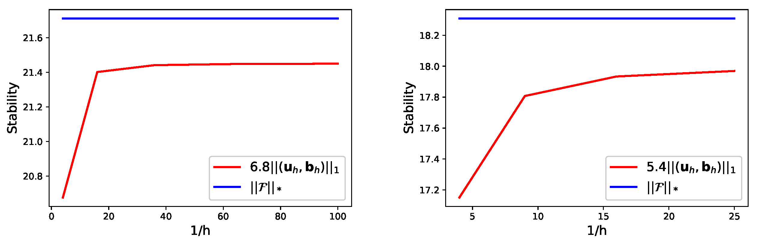
1/16	1/4	5.38 $\times {10}^{-3}$	1.98	2.99 $\times {10}^{-1}$	1.00	1.12 $\times {10}^{-1}$	1.86	189.50

and

Table 6. Convergence of ${\mathbf{b}}_h$ and $r_h$ (first class Nédélec element).

h	H	$\left|\right|\mathit{b}-{\mathit{b}}_{\mathit{h}}{\left|\right|}_0$	order	$\left|\right|\mathit{b}-{\mathit{b}}_{\mathit{h}}{\left|\right|}_{\mathbf{curl}}$	order	$\left|\right|\mathit{r}-{\mathit{r}}_{\mathit{h}}{\left|\right|}_0$	CPU(s)
SFEM	1/4	1.38 $\times {10}^{-1}$		8.38 $\times {10}^{-1}$		7.86 $\times {10}^{-16}$	2.03
1/4	1/2	1.38 $\times {10}^{-1}$		8.39 $\times {10}^{-1}$		9.82 $\times {10}^{-16}$	1.44
SFEM	1/9	6.16 $\times {10}^{-2}$	1.00	3.81 $\times {10}^{-1}$	0.97	4.24 $\times {10}^{-15}$	28.05
1/9	1/3	6.17 $\times {10}^{-2}$	0.99	3.83 $\times {10}^{-1}$	0.96	4.71 $\times {10}^{-15}$	16.26
SFEM	1/16	3.47 $\times {10}^{-2}$	1.00	2.14 $\times {10}^{-1}$	1.00	1.59 $\times {10}^{-14}$	577.84
1/16	1/4	3.47 $\times {10}^{-2}$	1.00	2.18 $\times {10}^{-1}$	0.98	1.42 $\times {10}^{-14}$	189.50

, the variable quantity $(\mathbf{u},\mathbf{b},p,r)$ is approximated by $P_1$, the first class Nédélec element, $P_1$ and $P_1$, respectively.

Table 7. Convergence of ${\mathbf{u}}_h$ and $p_h$ (second class Nédélec element).

h	H	$\left|\right|\mathit{u}-{\mathit{u}}_{\mathit{h}}{\left|\right|}_0$	order	$\left|\right|\mathit{\nabla }(\mathit{u}-{\mathit{u}}_{\mathit{h}}){\left|\right|}_0$	order	$\left|\right|\mathit{p}-{\mathit{p}}_{\mathit{h}}{\left|\right|}_0$	order	CPU(s)
SFEM	1/4	7.86 $\times {10}^{-2}$		1.17		1.39		2.39
1/4	1/2	7.86 $\times {10}^{-2}$		1.17		1.40		1.85
SFEM	1/9	1.67 $\times {10}^{-2}$	1.91	5.33 $\times {10}^{-1}$	0.97	3.26 $\times {10}^{-1}$	1.79	99.42
1/9	1/3	1.67 $\times {10}^{-2}$	1.91	5.34 $\times {10}^{-1}$	0.97	3.30 $\times {10}^{-1}$	1.78	42.96
SFEM	1/16	\	\	\	\	\	\	\
1/16	1/4	5.35 $\times {10}^{-3}$	1.98	2.99 $\times {10}^{-1}$	1.00	1.11 $\times {10}^{-1}$	1.86	2877.53

and

Table 8. Convergence of ${\mathbf{b}}_h$ and $r_h$ (second class Nédélec element).

h	H	$\left|\right|\mathit{b}-{\mathit{b}}_{\mathit{h}}{\left|\right|}_0$	order	$\left|\right|\mathit{b}-{\mathit{b}}_{\mathit{h}}{\left|\right|}_{\mathbf{curl}}$	order	$\left|\right|\mathit{r}-{\mathit{r}}_{\mathit{h}}{\left|\right|}_0$	CPU(s)
SFEM	1/4	6.64 $\times {10}^{-2}$		8.29 $\times {10}^{-1}$		8.89 $\times {10}^{-16}$	2.39
1/4	1/2	6.64 $\times {10}^{-2}$		8.30 $\times {10}^{-1}$		1.10 $\times {10}^{-15}$	1.85
SFEM	1/9	1.40 $\times {10}^{-2}$	1.91	3.76 $\times {10}^{-1}$	0.98	5.60 $\times {10}^{-15}$	99.42
1/9	1/3	1.41 $\times {10}^{-2}$	1.91	3.76 $\times {10}^{-1}$	0.97	6.19 $\times {10}^{-15}$	42.96
SFEM	1/16	\	\	\	\	\	\
1/16	1/4	4.61 $\times {10}^{-3}$	1.95	2.12 $\times {10}^{-1}$	1.00	2.26 $\times {10}^{-14}$	2877.53

list the results when $(\mathbf{u},\mathbf{b},p,r)$ is approximated by $P_1$, the second class Nédélec element, $P_1$ and $P_1$. It is observed that the numerical results agree well with the theoretical results of Theorems 1–3. On the other hand, from Table 7 and Table 8, we find that SFEM (35) does not work when $H=1/16$, however two-level SFEM (41) and (42) is valid in the current computing environment for our computer. On the other hand, the stability results of (43) are checked by Figure 1.

2D MHD problem with a singular solution: We consider 2D MHD system (1) in the L-type domain $\Omega :={[-1,1]}^2\backslash ([0,1]\times [-1,0])$. Set $R_e=S=1,R_m=0.001$, the analytical solution in polar coordinates $(\rho ,\phi )$ is given by [40]

$$\left\{\begin{array}{cc}\hfill \mathbf{u}(\rho ,\phi )& =\left[\begin{array}{c}{\rho }^{\lambda }\left((1+\lambda )sin\left(\phi \right)\psi \left(\varphi \right)+cos\left(\phi \right){\psi }^{\prime }\left(\phi \right)\right)\hfill \\ {\rho }^{\lambda }\left(-(1+\lambda )cos\left(\phi \right)\psi \left(\phi \right)+sin\left(\phi \right){\psi }^{\prime }\left(\phi \right)\right)\hfill \end{array}\right],\hfill \\ \hfill \mathbf{b}(\rho ,\phi )& =\nabla \left({\rho }^{2/3}sin(2/3\phi )\right),\hfill \\ \hfill p(\rho ,\phi )& =-{\rho }^{\lambda -1}\left({(1+\lambda )}^2{\psi }^{\prime }\left(\phi \right)+{\psi }^{‴}\left(\phi \right)\right)/(1-\lambda ),\hfill \\ \hfill r& =0,\hfill \\ \hfill \psi \left(\phi \right)& =sin\left(\right(1+\lambda \left)\phi \right)cos\left(\lambda \omega \right)/(1+\lambda )-cos\left(\right(1+\lambda \left)\phi \right)\hfill \\ \hfill & -sin\left(\right(1-\lambda \left)\phi \right)cos\left(\lambda \omega \right)/(1-\lambda )+cos\left(\right(1-\lambda \left)\phi \right),\hfill \\ \hfill \omega & =\frac{3}{2}\pi ,\hfill \\ \hfill \lambda & \approx 0.54448373678246.\hfill \end{array}\right.$$

In the 2D case, there holds the regularity $\mathbf{u}\in {\mathbf{H}}^{1+\lambda }(\Omega )$, $\mathbf{b}\in {\mathbf{H}}^{\frac{2}{3}}(\Omega )$ and $p\in H^{\lambda }(\Omega )$.

In

Table 9. Convergence of ${\mathbf{u}}_h$ and $p_h$.

h	H	$\left|\right|\mathit{u}-{\mathit{u}}_{\mathit{h}}{\left|\right|}_0$	order	$\left|\right|\mathit{\nabla }(\mathit{u}-{\mathit{u}}_{\mathit{h}}){\left|\right|}_0$	order	$\left|\right|\mathit{p}-{\mathit{p}}_{\mathit{h}}{\left|\right|}_0$	order	CPU(s)
SFEM	1/4	9.97 $\times {10}^{-2}$		1.55		1.74		0.16
1/4	1/2	9.96 $\times {10}^{-2}$		1.55		1.76		0.16
SFEM	1/16	1.27 $\times {10}^{-2}$	1.48	7.41 $\times {10}^{-1}$	0.54	7.74 $\times {10}^{-1}$	0.59	1.89
1/16	1/4	1.29 $\times {10}^{-2}$	1.47	7.41 $\times {10}^{-1}$	0.54	7.80 $\times {10}^{-1}$	0.59	1.11
SFEM	1/36	3.95 $\times {10}^{-3}$	1.45	4.78 $\times {10}^{-1}$	0.54	5.00 $\times {10}^{-1}$	0.54	12.03
1/36	1/6	4.06 $\times {10}^{-3}$	1.43	4.78 $\times {10}^{-1}$	0.54	5.22 $\times {10}^{-1}$	0.49	6.04
SFEM	1/64	1.77 $\times {10}^{-3}$	1.39	3.50 $\times {10}^{-1}$	0.54	3.76 $\times {10}^{-1}$	0.49	49.61
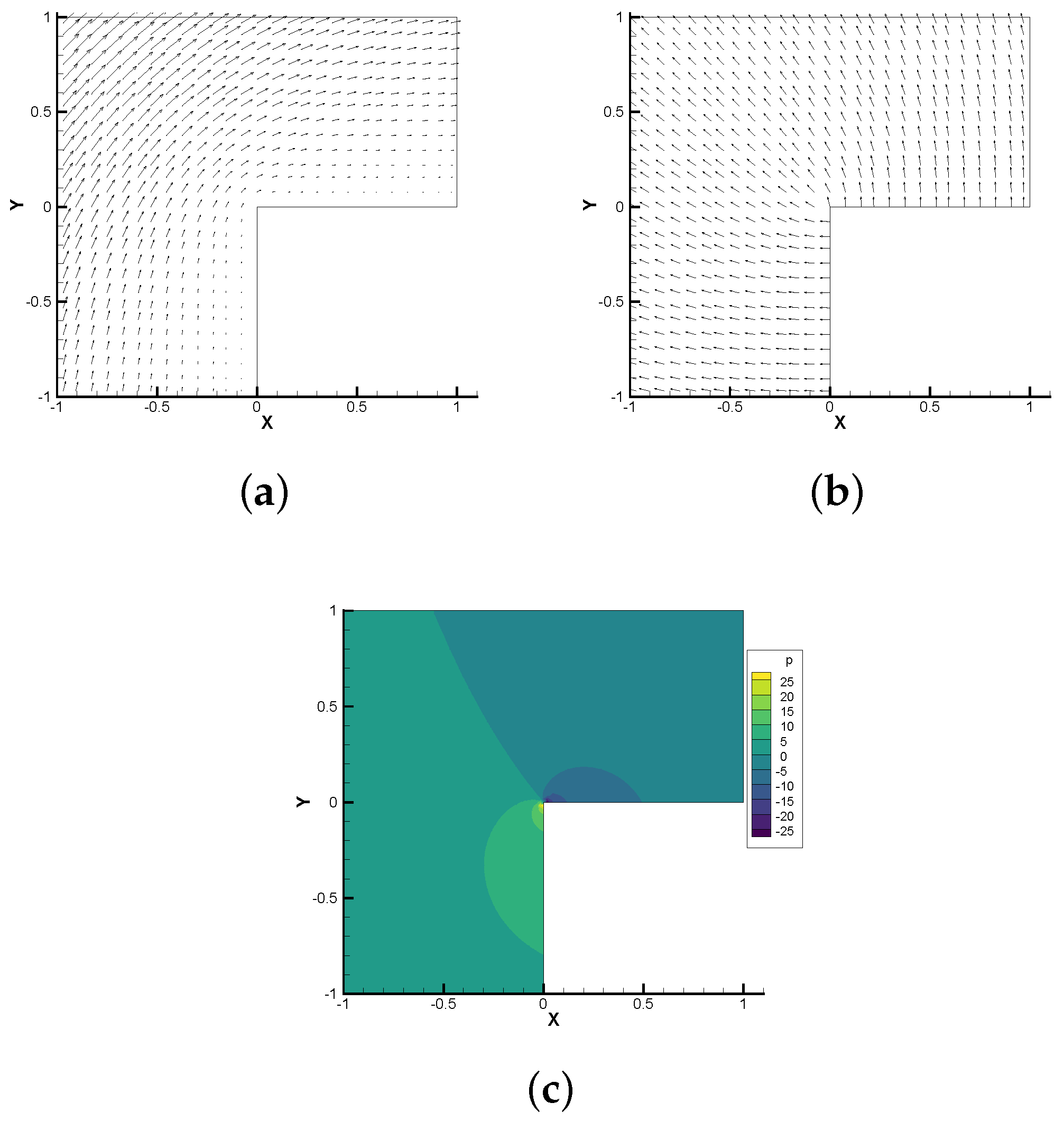
1/64	1/8	1.84 $\times {10}^{-3}$	1.37	3.50 $\times {10}^{-1}$	0.54	3.93 $\times {10}^{-1}$	0.49	22.80

and

Table 10. Convergence of ${\mathbf{b}}_h$ and $r_h$.

h	H	$\left|\right|\mathit{b}-{\mathit{b}}_{\mathit{h}}{\left|\right|}_0$	order	$\left|\right|\mathit{b}-{\mathit{b}}_{\mathit{h}}{\left|\right|}_{\mathbf{curl}}$	order	$\left|\right|\mathit{r}-{\mathit{r}}_{\mathit{h}}{\left|\right|}_0$	CPU(s)
SFEM	1/4	1.91 $\times {10}^{-1}$		1.91 $\times {10}^{-1}$		5.98 $\times {10}^{-4}$	0.16
1/4	1/2	1.90 $\times {10}^{-1}$		1.91 $\times {10}^{-1}$		5.98 $\times {10}^{-4}$	0.16
SFEM	1/16	7.88 $\times {10}^{-2}$	0.64	7.88 $\times {10}^{-2}$	0.64	1.47 $\times {10}^{-4}$	1.89
1/16	1/4	7.88 $\times {10}^{-2}$	0.64	7.88 $\times {10}^{-2}$	0.64	1.47 $\times {10}^{-4}$	1.11
SFEM	1/36	4.63 $\times {10}^{-2}$	0.65	4.63 $\times {10}^{-2}$	0.65	5.84 $\times {10}^{-5}$	12.03
1/36	1/6	4.63 $\times {10}^{-2}$	0.65	4.63 $\times {10}^{-2}$	0.65	5.84 $\times {10}^{-5}$	6.04
SFEM	1/64	3.17 $\times {10}^{-2}$	0.66	3.17 $\times {10}^{-2}$	0.66	2.97 $\times {10}^{-5}$	49.61
1/64	1/8	3.17 $\times {10}^{-2}$	0.66	3.17 $\times {10}^{-2}$	0.66	2.97 $\times {10}^{-5}$	22.80

, $(\mathbf{u},\mathbf{b},p,r)$ is approximated by $P_1$, the second class Nédélec element, $P_1$ and $P_1$. Because the regularity of velocity, magnetic field and pressure is low, the convergence of $\left|\right|\mathbf{u}-{\mathbf{u}}_h{\left|\right|}_0$, $\left|\right|\nabla (\mathbf{u}-{\mathbf{u}}_h){\left|\right|}_0$, $\left|\right|p-p_h{\left|\right|}_0$, $\left|\right|\mathbf{b}-{\mathbf{b}}_h{\left|\right|}_0$, $\left|\right|\mathbf{b}-{\mathbf{b}}_h{\left|\right|}_{\mathrm{curl}}$ keep the rate of 1.4, 0.54, 0.59, 0.66, 0.66, respectively, which verify the correctness of the theoretical analysis (Theorems 2 and 3) results. In Figure 2 we display the streamlines of the velocity field and magnetic field, and the contours of the pressure, which are consistent with the numerical results in the literature [40].

5. Conclusions

Based on the stabilization and the Lagrange multiplier techniques, the stabilized finite element algorithm is designed for the stationary incompressible MHD. The Lagrange multiplier technique idea helps us in dealing with the low regular magnetic field sub-problem by $H(curl;\Omega )$-conforming element. The stabilized one by using local Gauss integration allow us to adopt the lowest equal-order elements to approximate the flow field sub-problem. The stability and optimal convergence analysis are given. Furthermore, the two-level stabilized finite element algorithms are presented. In the first step we combine the stabilized finite element method with the Oseen iteration for the nonlinear MHD equations on a coarse grid. For the second step, we employ the linearized correction on a fine grid. We give the optimal error analysis, which shows that when the grid sizes satisfy $h=O\left(H^2\right)$, the two-level stabilization method not only has the optimal convergence order, but also can save more computational cost than the one-level method. These theoretical analysis results have been verified by some numerical experiments.

References

- Gerbeau, J.; Le Bris, C.; Lelièvre, T. Mathematical Methods for the Magnetohydrodynamics of Liquid Metals; Clarendon Press: Oxford, UK, 2006. [Google Scholar]
- Gunzburger, M.; Meir, A.; Peterson, J. On the existence, uniqueness, and finite element approximation of solutions of the equations of stationary, incompressible magnetohydrodynamics. Math. Comput. 1991, 56, 523–563. [Google Scholar] [CrossRef]
- Shi, D.; Yu, Z. Nonconforming mixed finite element methods for stationary incompressible magnetohydrodynamics. Int. J. Numer. Anal. Model. 2013, 10, 904–919. [Google Scholar]
- Dong, X.; He, Y.; Zhang, Y. Convergence analysis of three finite element iterative methods for the 2D/3D stationary incompressible magnetohydrodynamics. Comput. Meth. Appl. Math. Eng. 2014, 276, 287–311. [Google Scholar] [CrossRef]
- Dong, X.; He, Y. The Oseen type finite element iterative method for the stationary incompressible magnetohydrodynamics. Adv. Appl. Math. Mech. 2017, 9, 775–794. [Google Scholar] [CrossRef]
- Mao, S.; Feng, X.; Su, H. Optimal error estimates of penalty based iterative methods for steady incompressible magnetohydrodynamics equations with different viscosities. J. Sci. Comput. 2019, 79, 1078–1110. [Google Scholar]
- Du, B.; Huang, J. The generalized Arrow-Hurwicz method with applications to fluid computation. Commun. Comput. Phys. 2019, 25, 752–780. [Google Scholar] [CrossRef] [Green Version]
- Layton, W.; Meir, A.; Schmidtz, P. A two-level discretization method for the stationary MHD equations. Electron. Trans. Numer. Anal. 1997, 6, 198–210. [Google Scholar]
- Su, H.; Xu, J.; Feng, X. Optimal convergence analysis of two-level nonconforming finite element iterative methods for 2D/3D MHD equations. Entropy 2022, 24, 587. [Google Scholar] [CrossRef]
- Su, H.; Feng, X.; Zhao, J. On two-level Oseen penalty iteration methods for the 2D/3D stationary incompressible magnetohydronamics. J. Sci. Comput. 2020, 83, 11. [Google Scholar] [CrossRef]
- Dong, X.; He, Y. Convergence of some finite element iterative methods related to different Reynolds numbers for the 2D/3D stationary incompressible magnetohydrodynamics. Sci. China Math. 2016, 59, 589–608. [Google Scholar] [CrossRef]
- Dong, X.; He, Y. Two-level Newton iterative method for the 2D/3D stationary incompressible magnetohydrodynamics. J. Sci. Comput. 2015, 63, 426–451. [Google Scholar] [CrossRef]
- Tang, Q.; Huang, Y. Local and parallel finite element algorithm based on Oseen-type iteration for the stationary incompressible MHD flow. J. Sci. Comput. 2017, 70, 149–174. [Google Scholar]
- Dong, X.; He, Y.; Wei, H.; Zhang, Y. Local and parallel finite element algorithm based on the partition of unity method for the incompressible MHD flow. Adv. Comput. Math. 2018, 44, 1295–1319. [Google Scholar] [CrossRef]
- Tang, Q.; Huang, Y. Analysis of local and parallel algorithm for incompressible magnetohydrodynamics flows by finite element iterative method. Commun. Comput. Phys. 2019, 25, 729–751. [Google Scholar] [CrossRef]
- Dong, X.; He, Y. A parallel finite element method for incompressible magnetohydrodynamics equations. Appl. Math. Lett. 2020, 102, 106076. [Google Scholar] [CrossRef]
- Li, L.; Zheng, W. A robust solver for the finite element approximation of stationary incompressible MHD equations in 3D. J. Comput. Phys. 2017, 351, 254–270. [Google Scholar] [CrossRef] [Green Version]
- Ma, Y.; Hu, K.; Hu, X.; Xu, J. Robust preconditioners for incompressible MHD models. J. Comput. Phys. 2016, 316, 721–746. [Google Scholar] [CrossRef] [Green Version]
- Zhang, G.; Yang, M.; He, Y. Block preconditioners for energy stable schemes of magnetohydrodynamics equations. Numer. Methods Partial Differ. Eq. 2022. [Google Scholar] [CrossRef]
- Li, L.; Zhang, D.; Zheng, W. A constrained transport divergence-free finite element method for incompressible MHD equations. J. Comput. Phys. 2021, 428, 109980. [Google Scholar] [CrossRef]
- Zhang, G.; He, Y.; Yang, D. Analysis of coupling iterations based on the finite element method for stationary magnetohydrodynamics on a general domain. Comput. Math. Appl. 2014, 68, 770–788. [Google Scholar] [CrossRef]
- Li, J.; He, Y. A stabilized finite element method based on two local Gauss integrations for the Stokes equations. J. Comput. Appl. Math. 2008, 214, 58–65. [Google Scholar] [CrossRef] [Green Version]
- Zheng, H.; Shan, L.; Hou, Y. A quadratic equal-order stabilized method for Stokes problem based on two local Gauss integrations. Numer. Methods Partial Differ. Eq. 2010, 26, 1180–1190. [Google Scholar] [CrossRef]
- Li, R.; Li, J.; Chen, Z. A stabilized finite element method based on two local Gauss integrations for a coupled Stokes-Darcy problem. J. Comput. Appl. Math. 2016, 292, 92–104. [Google Scholar] [CrossRef]
- Huang, P.; He, Y.; Feng, X. Two-level stabilized finite element method for Stokes eigenvalue problem. Appl. Math. Mech. 2012, 33, 621–630. [Google Scholar] [CrossRef]
- Li, J. Investigations on two kinds of two-level stabilized finite element methods for the stationary Navier-Stokes equations. Appl. Math. Comput. 2006, 182, 1470–1481. [Google Scholar] [CrossRef]
- Li, J.; He, Y.; Chen, Z. A new stabilized finite element method for the transient Navier-Stokes equations. Comput. Meth. Appl. Math. Eng. 2007, 197, 22–35. [Google Scholar] [CrossRef]
- He, Y.; Li, J. A stabilized finite element method based on local polynomial pressure projection for the stationary Navier-Stokes equations. Appl. Numer. Math. 2008, 58, 1503–1514. [Google Scholar] [CrossRef]
- Jiang, Y.; Mei, L.; Wei, H. A stabilized finite element method for transient Navier-Stokes equations based on two local Gauss integrations. Int. J. Numer. Meth. Fluids 2012, 70, 713–723. [Google Scholar] [CrossRef]
- Huang, P.; Zhao, J.; Feng, X. Highly efficient and local projection-based stabilized finite element method for natural convection problem. Int. J. Heat Mass Tran. 2015, 83, 357–365. [Google Scholar] [CrossRef]
- Schötzau, D. Mixed finite element methods for stationary incompressible magnetohydrodynamics. Numer. Math. 2004, 96, 771–800. [Google Scholar] [CrossRef]
- Heywood, J.; Rannacher, R. Finite-element approximation of the nonstationary Navier-Stokes problem. Part IV: Error analysis for second-order time discretization. SIAM J. Numer. Anal. 1990, 27, 353–384. [Google Scholar] [CrossRef]
- Sermange, M.; Temam, R. Some mathematical questions related to the MHD equations. Comm. Pure Appl. Math. 1984, 34, 635–664. [Google Scholar]
- He, Y.; Zhang, G.; Zou, J. Fully discrete finite element approximation of the MHD flow. Comput. Methods Appl. Math. 2022, 22, 357–388. [Google Scholar] [CrossRef]
- Nédélec, J. A new family of mixed finite elements in R3. Numer. Math. 1986, 50, 57–81. [Google Scholar] [CrossRef]
- Girault, V.; Raviart, P. Finite Element Approximation of the Navier-Stokes Equations; Springer: Berlin/Heidelberg, Germany, 1979. [Google Scholar]
- Monk, P. Finite Element Methods for Maxwell’s Equations; Oxford University Press: Oxford, UK, 2003. [Google Scholar]
- Huang, P.; Feng, X.; He, Y. Two-level defect-correction Oseen iterative stabilized finite element methods for the stationary Navier-Stokes equations. Appl. Math. Model. 2013, 37, 728–741. [Google Scholar] [CrossRef]
- FEALPy Help and Installation. Available online: https://www.weihuayi.cn/fly/fealpy.html (accessed on 24 March 2022).
- Greif, C.; Li, D.; Schötzau, D.; Wei, X. A mixed finite element method with exactly divergence-free velocities for incompressible magnetohydrodynamics. Comput. Meth. Appl. Math. Eng. 2010, 199, 2840–2855. [Google Scholar] [CrossRef]
- Layton, W.; Lee, H.; Peterson, J. A defect-correction method for the incompressible Navier-Stokes equations. Appl. Math. Comput. 2002, 129, 1–19. [Google Scholar] [CrossRef]
Figure 1.
Stability of 2D (left) and 3D (right) problems.
Figure 2.
Numerical approximations of 2D singular solution. (a) velocity field; (b) magnetic field; (c) pressure.