Article

Robust Finite-Time Stability for Uncertain Discrete-Time Stochastic Nonlinear Systems with Time-Varying Delay

1
College of Mathematics and Systems Science, Shandong University of Science and Technology, Qingdao 266590, China
2
Department of Fundamental Courses, Shandong University of Science and Technology, Jinan 250031, China
*
Author to whom correspondence should be addressed.
These authors contributed equally to this work.
Entropy 2022, 24(6), 828; https://doi.org/10.3390/e24060828
Submission received: 8 May 2022 / Revised: 10 June 2022 / Accepted: 11 June 2022 / Published: 14 June 2022

Abstract

:
The main concern of this paper is finite-time stability (FTS) for uncertain discrete-time stochastic nonlinear systems (DSNSs) with time-varying delay (TVD) and multiplicative noise. First, a Lyapunov–Krasovskii function (LKF) is constructed, using the forward difference, and less conservative stability criteria are obtained. By solving a series of linear matrix inequalities (LMIs), some sufficient conditions for FTS of the stochastic system are found. Moreover, FTS is presented for a stochastic nominal system. Lastly, the validity and improvement of the proposed methods are shown with two simulation examples.

1. Introduction

Time-delays are general in many actual systems, for instance, circuits, neural network systems, biological medicine, building structure and multi-agent systems [1,2,3,4]. However, a time-delay may reduce the performance of dynamic systems and even lead to system instability. Therefore, how to eliminate the adverse effects caused by time-delay on the system is an important consideration. A new Lyapunov method was proposed to study the stability of the system [5]. In [6], Zhang et al. introduced a reciprocally convex matrix inequality to analyze the stability of TVD systems. A FTS or stabilization criterion was given for linear time-delay systems (TDSs) through bounded linear time-varying feedback [7]. The practical stability of TVD-positive systems was analyzed by designing a controller [8]. Long et al. considered the stability of linear TDS via the quadratic function negative deterministic method [9].
In actual engineering, it is common for the system to be interfered with by some nonlinear factors. The control analysis of nonlinear TDSs becomes more important. In order to obtain a greater upper limit of TVD, a new less-conservative stability criterion for nonlinear perturbed TDS was proposed in [10]. The authors of [11] developed robust stability of switching systems with nonlinear disturbances and interval TVD. Finite-time control problems for nonlinear systems with TVD and external interference were discussed in [12]. In general, there is often uncertainty in the parameters of the system model. Kang et al. [13] studied the FTS of discrete-time nonlinear systems with interval TVD. On the basis of [13], Stojanovic proposed a less conservative FTS criterion for discrete-time nonlinear systems with TVD and uncertain terms [14].
The most basic concepts of system stability include FTS [15,16,17] and Lyapunov asymptotic stability (LAS) [18,19]. FTS and LAS are different in two ways. First, FTS studies the state behavior of a system within a limited time interval, and LAS studies the state behavior of a system in an infinite time interval. Secondly, the former research needs to give the limit of the system state in advance, while the latter does not need to give a fixed value in advance. In [20], Dorato introduced the concept of FTS. In a sense, if the state of the system under the initial condition does not exceed the specified range, then the system is called FTS within a certain time interval. In recent years, the research on FTS has attracted much attention. Thus far, many new results on FTS have been published. Shi et al. extended the discrete Jensen-based inequality by establishing a new weighted summation inequality and proposed new criteria for the FTS of nonlinear TDS [21]. The concepts of FTS and stabilization are extended to continuous additive TVD systems [22].
In the above-mentioned literature, the dynamic systems are definite; however, in the actual industrial production process, random phenomena are widespread [23]. From the perspective of theory or practical application, the control problem of stochastic systems is always a difficult issue. In [24], Yu et al. studied the FTS and H control problem for stochastic nonlinear systems. Wang et al. discussed the FTS of stochastic nonlinear systems by constructing Hamiltonian functions [25]. The stochastic FTS of linear semi-Markov jump systems was developed by designing a class of state feedback controllers [26].
Yan et al. proposed a less conservative stability criterion through a model-dependent method and gave the FTS and stabilization conditions of Markov jump I t o ^ stochastic systems [27]. The authors in [28] considered the FTS problem of stochastic linear discrete-time TDS with multiplicative noise under state feedback control [29] discussed the finite-time guaranteed performance control of random mean-field systems and gave the criterion of FTS for the closed-loop system. However, there is no literature to discuss the FTS of uncertain DSNS with multiplicative noise and time-delay.
The results of FTS are extended to uncertain DSNS with TVD in this paper. The followings are the major contributions: First, a new augmented time-varying LKF is proposed, which contains a power function ζ k j 1 . A special finite sum inequality (NFSI) is used to process the forward difference of LKF with double summation terms. This NFSI is equivalent to Jensen’s inequality but reduces conservatism to a certain extent. Secondly, one-dimensional random processes, namely a sequence of one-dimensional independent white noise processes defined in probability space ( Ω , F , P , F n ) , are considered as an external disturbance of the system. An algorithm is presented to reduce the influence of external interference on the stability of uncertain DSNS.
In addition, the uncertain parameters and nonlinear perturbations are transformed into linearity through the inequality calculation. The remainder is arranged as follows: some preparatory knowledge for the discrete-time stochastic system, the requisite lemmas and definitions are given in Section 2. The FTS of discrete time-varying stochastic uncertain system with nonlinear perturbations is studied, and then the FTS of a nominal system is considered in Section 3. By constructing an LKF with a power function and a new summation term, the criteria to guarantee the FTS of the discrete-time stochastic system are given. Simulation examples are presented to demonstrate the validity of the results in Section 4. Section 5 is the conclusion of this paper.
Notation: In this paper, R n means the n-dimensional Euclidean space, R n × m is all real matrices with dimensions of n × m . N 0 = { h M , h M + 1 , , 1 , 0 } , N = { 1 , 2 , 3 , , N } . For matrix P R n × m , λ m a x ( P ) represents the maximum eigenvalue, and λ m i n ( P ) denotes the minimum eigenvalue of matrix P. P > 0 ( P 0 ) means P is positive definite (positive semi-definite) matrix. The ∗ sign in the matrix indicates the symmetry item.

2. Problem Statement and Preliminaries

Consider an uncertain DSNS with TVD as follows
x ( k + 1 ) = ( M + Δ M ( k ) ) x ( k ) + ( M d + Δ M d ( k ) ) x ( k h ( k ) ) + e 1 ( x ( k ) , k ) + e 2 ( x ( k h ( k ) ) , k ) + D x ( k ) ω ( k ) , x ( l ) = φ ( l ) , l N 0 ,
where x ( k ) R n is the state vector, ω ( k ) is a one-dimensional random variable defined on the probability space ( Ω , F , P , F n ) . M , M d , D R n × n are constant matrices with appropriate dimensions. It is supposed that E { ω ( l ) } = 0 , E { ω ( l ) ω ( k ) } = δ l k , when l k , δ l k = 0 ; when l = k , δ l k = 1 , where E { · } represents mathematical expectation, and δ l k is a Kronecker function. h ( k ) is the interval TVD and satisfies 0 < h m h ( k ) h M . φ ( l ) is a vector-valued initial sequence such that
sup l N 0 ( φ ( l + 1 ) φ ( l ) ) T ( φ ( l + 1 ) φ ( l ) ) δ .
e 1 ( x ( k ) , k ) and e 2 ( x ( k h ( k ) ) , k ) are nonlinear disturbances, and H and H d are known constant matrices satisfying
e 1 T ( x ( k ) , k ) e 1 ( x ( k ) , k ) x T ( k ) H T H x ( k ) , e 2 T ( x ( k h ( k ) ) , k ) e 2 ( x ( k h ( k ) ) , k ) x T ( k h ( k ) ) H d T H d x ( k h ( k ) ) .
Δ M ( k ) , Δ M d ( k ) and Δ ( k ) are unknown time-varying matrices that are uniformly bounded in the norm. F, F d and G are known matrices with
Δ M ( k ) Δ M d ( k ) = G Δ ( k ) F F d , Δ T ( k ) Δ ( k ) I .
Let z ( k ) represent an unknown variable, and the system (1) can be written as follows:
x ( k + 1 ) = M x ( k ) + M d x ( k h ( k ) ) + G z ( k ) + e 1 ( x ( k ) , k ) + e 2 ( x ( k h ( k ) ) , k ) + D x ( k ) ω ( k ) , z ( k ) = Δ ( k ) ( F x ( k ) + F d x ( k h ( k ) ) ) , x ( l ) = φ ( l ) , l N 0 .
For system (1), if the perturbations and uncertainties are not considered, it can be expressed as:
x ( k + 1 ) = M x ( k ) + M d x ( k h ( k ) ) + D x ( k ) ω ( k ) , x ( l ) = φ ( l ) , l N 0 ,
which is called a nominal system.
In order to analyze the FTS of system (1), the following definition and lemmas are introduced.
Definition 1.
For given scalars 0 α β , system (1) is FTS subject to ( α , β , N ) , n N , if
sup l N 0 φ ( l ) 2 α E { x ( k ) 2 } < β .
Remark 1.
It is worth noting that α and β are all used to describe the state variables remain on the given limits. β is influenced by α as a parameter adjustment in the simulation; however, that does not mean that β only depends on α. In addition, different from the plain stability, the characteristics of finite-time stability are as follows: First, the initial condition is confined to a prescribed limit. Second, the state trajectory does not exceed the specified value over a finite-time interval instead of an infinite-time interval.
Remark 2.
Compared with the continuous-time system [30,31,32], the FTS of the discrete-time stochastic systems [33,34,35] has received much less attention because the analysis can be simplified to the robust stability of linear systems with uncertainties but no delay. That is to say, in the discrete-time case, the presence of time-delay can be modeled by extending the system state with past variables, i.e., X ( k ) = [ x ( k ) , x ( k 1 ) , · · · , x ( k h M ) ] T . However, the optimization algorithms are easier to complete on the computer as well as the growing applications in certain engineering fields; therefore, the stability analysis of discrete-time stochastic systems is meaningful. In the next sections, we extend the analysis of FTS to stochastic systems.
Lemma 1
([36]). For any matrices with appropriate dimensions L > 0 , L T > 0 , L R m × m , S R n × m , scalar ζ > 0 and h 1 , h 2 N , h 2 > h 1 , the following inequality holds
j = k h 2 k h 1 1 ζ k j y T ( j ) L y ( j ) ξ T ( k ) ε S L 1 S T ξ ( k ) + 2 ξ T ( k ) S ( x ( k h 1 ) x ( k h 2 ) ) ,
where y ( j ) = x ( j + 1 ) x ( j ) , ξ ( k ) R n × 1 is the state vector and ε > 0 is a constant defined as follows
ε = h 2 h 1 , ζ = 1 , ( ζ h 1 ζ h 2 ) / ( ζ 1 ) , ζ 1 .
Lemma 2
([37]). (Schur complement) For the given symmetric matrix T = T 11 T 12 T 22 , where T 11 R n × n , the following three conditions are equivalent:
( 1 ) T < 0 ; ( 2 ) T 11 < 0 , T 22 T 12 T T 11 1 T 12 < 0 ; ( 3 ) T 22 < 0 , T 11 T 12 T 22 1 T 12 T < 0 .

3. Main Results

In this section, the FTS and RAS problems for system (1) are discussed, and the FTS criteria for the nominal system (2) are presented.

3.1. FTS for Stochastic Systems with Nonlinear Disturbances and Uncertain Parameters

In this section, stochastic system (1) is considered with uncertain parameters and nonlinear disturbances, the sufficient conditions of FTS for system (1) are given first.
Theorem 1.
Given constant ζ > 1 and positive constants ϵ , ϵ d , μ , λ 1 , λ 2 , , λ 8 , then the uncertain DSNS (1) with TVD is FTS subject to { α , β , N } if there exist matrices A = [ A 1 T A 2 T A 7 T ] T , B = [ B 1 T B 2 T B 7 T ] T and C = [ C 1 T C 2 T C 7 T ] T as well as positive definite matrices P , W 1 , W 2 , Q 1 , Q 2 R n × n , such that all of the following conditions hold:
[ Θ i j ] i , j = 1 , 2 , , 7 ε 1 A ε 1 B ε 2 C ε 1 Q 1 0 0 ε 1 Q 1 0 ε 2 Q 2 < 0 ,
λ 1 I < P < λ 2 I , λ 3 I < W 1 < λ 4 I , λ 5 I < W 2 < λ 6 I , Q 1 < λ 7 I , Q 2 < λ 8 I ,
ζ N [ α ( λ 2 + η 1 λ 4 + η 2 λ 6 ) + δ ( η 3 λ 7 + η 4 λ 8 ) ] β [ λ 1 + η 1 λ 3 + η 2 λ 5 ] < 0 ,
where
Θ 11 = M T P M ζ P + W 1 + W 2 + ( M I ) T Q 12 ( M I ) + ϵ H T H + μ F T F + C 1 + C 1 T + D T P D + D T Q 12 D , Θ 12 = M T P M d + ( M I ) T Q 12 M d + μ F T F d + A 1 B 1 + C 2 T , Θ 13 = B 1 C 1 + C 3 T , Θ 14 = A 1 + C 4 T , Θ 15 = M T P G + ( M I ) T Q 12 G + C 5 T , Θ 16 = M T P + ( M I ) T Q 12 + C 6 T , Θ 17 = M T P + ( M I ) T Q 12 + C 7 T , Θ 22 = M d T P M d + M d T Q 12 M d + ϵ d H d T H d + μ F d T F d + A 2 + A 2 T B 2 B 2 T , Θ 23 = A 3 T + B 2 B 3 T C 2 , Θ 24 = A 2 + A 4 T B 4 T , Θ 25 = M d T P G + M d T Q 12 G + A 5 T B 5 T , Θ 26 = M d T P + M d T Q 12 + A 6 T B 6 T , Θ 27 = M d T P + M d T Q 12 + A 7 T B 7 T , Θ 33 = ζ h m W 2 + B 3 + B 3 T C 3 C 3 T , Θ 34 = A 3 + B 4 T C 4 T , Θ 35 = B 5 T C 5 T , Θ 36 = B 6 T C 6 T , Θ 37 = B 7 T C 7 T , Θ 44 = ζ h M W 1 A 4 A 4 T , Θ 45 = A 5 T , Θ 46 = A 6 T , Θ 47 = A 7 T , Θ 55 = G T P G + G T Q 12 G μ I , Θ 56 = G T P + G T Q 12 , Θ 57 = G T P + G T Q 12 , Θ 66 = P + Q 12 ϵ I , Θ 67 = P + Q 12 , Θ 77 = P + Q 12 ϵ d I , Q 12 = ( h M h m ) Q 1 + h m Q 2 ,
ε 1 = h M h m , ζ = 1 , ( ζ h m ζ h M ) / ( ζ 1 ) , ζ 1 , ε 2 = h m , ζ = 1 , ( 1 ζ h m ) / ( ζ 1 ) , ζ 1 .
η 1 = h M , ζ = 1 , ( ζ h M 1 ) / ( ζ 1 ) , ζ 1 , η 2 = h m , ζ = 1 , ( ζ h m 1 ) / ( ζ 1 ) , ζ 1 , η 3 = h M ( h M + 1 ) 2 h m ( h m + 1 ) 2 , ζ = 1 , ( ζ h M + 1 ζ h m + 1 ( ζ 1 ) ( h M h m ) ) / ( ζ 1 ) 2 , ζ 1 , η 4 = h m ( h m + 1 ) 2 , ζ = 1 , ( ζ ( ζ h m 1 ) ( ζ 1 ) h m ) / ( ζ 1 ) 2 , ζ 1 .
Proof. 
Consider the following LKF ( k N ) ,
V ( k ) = s = 1 3 V s ( k ) ,
where
V 1 ( k ) = x T ( k ) P x ( k ) , V 2 ( k ) = j = k h M k 1 ζ k j 1 x T ( j ) W 1 x ( j ) + j = k h m k 1 ζ k j 1 x T ( j ) W 2 x ( j ) , V 3 ( k ) = i = h M h m 1 j = k + i k 1 ζ k j 1 y T ( j ) Q 1 y ( j ) + i = h m 1 j = k + i k 1 ζ k j 1 y T ( j ) Q 2 y ( j ) .
Along the trajectory of system (1), the forward differences of V 1 ( k ) , V 2 ( k ) and V 3 ( k ) are obtained as follows
E { Δ V 1 ( k ) } = E V 1 ( k + 1 ) V 1 ( k ) = E x T ( k + 1 ) P x ( k + 1 ) + ( ζ 1 ) V 1 ( k ) ζ V 1 ( k ) = E x T ( k ) ( M T P M + D T P D ζ P ) x ( k ) + ( ζ 1 ) V 1 ( k ) + 2 x T ( k ) M T P M d x ( k h ( k ) ) + 2 x T ( k ) M T P G z ( k ) + 2 x T ( k ) M T P e 1 ( x ( k ) , k ) + 2 x T ( k ) M T P e 2 ( x ( k h ( k ) ) , k ) + x T ( k h ( k ) ) M d T P M d x ( k h ( k ) ) + 2 x T ( k h ( k ) ) M d T P G z ( k ) + 2 x T ( k h ( k ) ) M d T P e 1 ( x ( k ) , k ) + z T ( k ) G T P G z ( k ) + 2 x T ( k h ( k ) ) M d T P e 2 ( x ( k h ( k ) ) , k ) + 2 z T ( k ) G T P e 1 ( x ( k ) , k ) + 2 z T ( k ) G T P e 2 ( x ( k h ( k ) ) , k ) + e 1 T ( x ( k ) , k ) P e 1 ( x ( k ) , k ) + 2 e 1 T ( x ( k ) , k ) P e 2 ( x ( k h ( k ) ) , k ) = + e 2 T ( x ( k h ( k ) ) , k ) P e 2 ( x ( k h ( k ) ) , k ) ,
E { Δ V 2 ( k ) } = E { V 2 ( k + 1 ) V 2 ( k ) } = E { j = k h M + 1 k ζ k j x T ( j ) W 1 x ( j ) + j = k h m + 1 k ζ k j x T ( j ) W 2 x ( j ) j = k h M k 1 ζ k j 1 x T ( j ) W 1 x ( j ) j = k h m k 1 ζ k j 1 x T ( j ) W 2 x ( j ) } = E { ζ j = k h M k 1 ζ k j 1 x T ( j ) W 1 x ( j ) + x T ( k ) W 1 x ( k ) ζ h M x T ( k h M ) W 1 x ( k h M ) + ζ j = k h m k 1 ζ k j 1 x T ( j ) W 2 x ( j ) + x T ( k ) W 2 x ( k ) ζ h m x T ( k h m ) W 2 x ( k h m ) V 2 ( k ) } = E ( ζ 1 ) V 2 ( k ) + x T ( k ) ( W 1 + W 2 ) x ( k ) ζ h M x T ( k h M ) W 1 x ( k h M ) ζ h m x T ( k h m ) W 2 x ( k h m ) ,
E { Δ V 3 ( k ) } = E { V 3 ( k + 1 ) V 3 ( k ) } = E { i = h M h m 1 j = k + i + 1 k ζ k j y T ( j ) Q 1 y ( j ) + i = h m 1 j = k + i + 1 k ζ k j y T ( j ) Q 2 y ( j ) i = h M h m 1 j = k + i k 1 ζ k j 1 y T ( j ) Q 1 y ( j ) i = h m 1 j = k + i k 1 ζ k j 1 y T ( j ) Q 2 y ( j ) } = E { i = h M h m 1 j = k + i k 1 ζ k j y T ( j ) Q 1 y ( j ) + i = h M h m 1 y T ( k ) Q 1 y ( k ) i = h M h m 1 ζ i y T ( k + i ) Q 1 y ( k + i ) + i = h m 1 j = k + i k 1 ζ k j y T ( j ) Q 2 y ( j ) + i = h m 1 y T ( k ) Q 2 y ( k ) i = h m 1 ζ i y T ( k + i ) Q 2 y ( k + i ) V 3 ( k ) } ,
then
E { Δ V 3 ( k ) } = E { ( h M h m ) y T ( k ) Q 1 y ( k ) j = k h M k h m 1 ζ k j y T ( j ) Q 1 y ( j ) + h m y T ( k ) Q 2 y ( k ) j = k h m k 1 ζ k j y T ( j ) Q 2 y ( j ) + ( ζ 1 ) V 3 ( k ) } = E { ( ζ 1 ) V 3 ( k ) + y T ( k ) [ ( h M h m ) Q 1 + h m Q 2 ] y ( k ) j = k h M k h m 1 ζ k j y T ( j ) Q 1 y ( j ) j = k h m k 1 ζ k j y T ( j ) Q 2 y ( j ) } .
From Lemma 1 and (13), we have
E j = k h M k h m 1 ζ k j y T ( j ) Q 1 y ( j ) = E j = k h M k h ( k ) 1 ζ k j y T ( j ) Q 1 y ( j ) j = k h ( k ) k h m 1 ζ k j y T ( j ) Q 1 y ( j ) E ξ T ( k ) ε 1 A Q 1 1 A T ξ ( k ) + 2 ξ T ( k ) A ( x ( k h ( k ) ) x ( k h M ) ) = + ξ T ( k ) ε 1 B Q 1 1 B T ξ ( k ) + 2 ξ T ( k ) B ( x ( k h m ) x ( k h ( k ) ) ) E ξ T ( k ) ε 1 A Q 1 1 A T ξ ( k ) + 2 ξ T ( k ) A 0 I 0 I 0 0 0 ξ ( k ) = + ξ T ( k ) ε 1 B Q 1 1 B T ξ ( k ) + 2 ξ T ( k ) B 0 I I 0 0 0 0 ξ ( k ) = E ξ T ( k ) ( Π 1 + ε 1 A Q 1 1 A T + ε 1 B Q 1 1 B T ) ξ ( k ) ,
E j = k h m k 1 ζ k j y T ( j ) Q 2 y ( j ) E ξ T ( k ) ε 2 C Q 2 1 C T ξ ( k ) + 2 ξ T ( k ) C ( x ( k ) x ( k h m ) ) = E ξ T ( k ) ε 2 C Q 2 1 C T ξ ( k ) + 2 ξ T ( k ) C I 0 I 0 0 0 0 ξ ( k ) = E ξ T ( k ) ( Π 2 + ε 2 C Q 2 1 C T ) ξ ( k ) ,
where
ξ ( n ) = [ x T ( k ) x T ( k h ( k ) ) x T ( k h m ) x T ( k h M ) z T ( k ) e 1 T ( x ( k ) , k ) e 2 T ( x ( k h ( k ) ) , k ) ] T ,
Π 1 = 0 Π 12 B 1 A 1 0 0 0 Π 22 Π 23 Π 24 A 5 T B 5 T A 6 T B 6 T A 7 T B 7 T B 3 + B 3 T A 3 + B 4 T B 5 T B 6 T B 7 T A 4 A 4 T A 5 T A 6 T A 7 T 0 0 0 0 0 0 ,
Π 12 = A 1 B 1 , Π 22 = A 2 B 2 + A 2 T B 2 T , Π 23 = B 2 + A 3 T B 3 T , Π 24 = A 2 + A 4 T B 4 T ,
Π 2 = C 1 + C 1 T C 2 T C 1 + C 3 T C 4 T C 5 T C 6 T C 7 T 0 C 2 0 0 0 0 C 3 C 3 T C 4 T C 5 T C 6 T C 7 T 0 0 0 0 0 0 0 0 0 0 , ε 1 = ( ζ h ( k ) ζ h M ) / ( ζ 1 ) ( ζ h m ζ h M ) / ( ζ 1 ) = ε 1 , ε 1 = ( ζ h m ζ h ( k ) ) / ( ζ 1 ) ( ζ h m ζ h M ) / ( ζ 1 ) = ε 1 .
From Equations (10)–(15) and condition (16)
ϵ x T ( k ) H T H x ( k ) ϵ e 1 T ( x ( k ) , k ) e 1 ( x ( k ) , k ) 0 , ϵ d x T ( k h ( k ) ) H d T H d x ( k h ( k ) ) ϵ d e 2 T ( x ( k h ( k ) ) , k ) e 2 ( x ( k h ( k ) ) , k ) 0 ,
we deduce that
E Δ V ( k ) E ( ζ 1 ) V ( k ) + x T ( k ) [ M T P M + D T P D ζ P + W 1 + W 2 + ( M I ) T Q 12 ( M I ) + D T Q 12 D ] x ( k ) + 2 x T ( k ) ( M T P M d + ( M I ) T Q 12 M d ) x ( k h ( k ) ) + 2 x T ( k ) ( M T P G + ( M I ) T Q 12 G ) z ( k ) + 2 x T ( k ) ( M T P + ( M I ) T Q 12 ) e 1 ( x ( k ) , k ) + 2 x T ( k ) ( M T P + ( M I ) T Q 12 ) e 2 ( x ( k h ( k ) ) , k ) + x T ( k h ( k ) ) ( M d T P M d + M d T Q 12 M d ) x ( k h ( k ) ) + 2 x T ( k h ( k ) ) ( M d T P G + M d T Q 12 G ) z ( k ) + 2 x T ( k h ( k ) ) ( M d T P + M d T Q 12 ) e 1 ( x ( k ) , k ) + 2 x T ( k h ( k ) ) ( M d T P + M d T Q 12 ) e 2 ( x ( k h ( k ) ) , k ) + z T ( k ) ( G T P G + G T Q 12 G ) z ( k ) + 2 z T ( k ) ( G T P + G T Q 12 ) e 1 ( x ( k ) , k ) + 2 z T ( k ) ( G T P + G T Q 12 ) e 2 ( x ( k h ( k ) ) , k ) + e 1 T ( x ( k ) , k ) ( P + Q 12 ) e 1 ( x ( k ) , k ) + 2 e 1 T ( x ( k ) , k ) ( P + Q 12 ) e 2 ( x ( k h ( k ) ) , k ) + e 2 T ( x ( k h ( k ) ) , k ) ( P + Q 12 ) e 2 ( x ( k h ( k ) ) , k ) ζ h M x T ( k h M ) W 1 x ( k h M ) ζ h m x T ( k h m ) W 2 x ( k h m ) + ξ T ( k ) ( Π 1 + Π 2 + ε 1 A Q 1 1 A T + ε 1 B Q 1 1 B T + ε 2 C Q 2 1 C T ) ξ ( k ) + ϵ x T ( k ) H T H x ( k ) ϵ e 1 T ( x ( k ) , k ) e 1 ( x ( k ) , k ) + ϵ d x T ( k h ( k ) ) H d T H d x ( k h ( k ) ) ϵ d e 2 T ( x ( k h ( k ) ) , k ) e 2 ( x ( k h ( k ) ) , k ) + μ x T ( k ) F T F x ( k ) 2 μ x T ( k ) F T F d x ( k h ( k ) ) + μ x T ( k h ( k ) ) F d T F d x ( k h ( k ) ) μ z T ( k ) z ( k ) ,
and it is rewritten that
E Δ V ( k ) E ( ζ 1 ) V ( k ) + ξ T ( k ) ( ( [ Θ i j ] i , j = 1 , 2 , , 7 ) + ε 1 A Q 1 1 A T = + ε 1 B Q 1 1 B T + ε 2 C Q 2 1 C T ) ξ ( k ) .
From Schur’s complement, (4) is equivalent to inequality (17)
( [ Θ i j ] i , j = 1 , 2 , , 7 ) + ε 1 A Q 1 1 A T + ε 1 B Q 1 1 B T + ε 2 C Q 2 1 C T < 0 .
Then,
E Δ V ( k ) ( ζ 1 ) V ( k ) < 0 ,
by calculating, one further finds
E V ( k ) < ζ k E V ( 0 ) , k N .
According to the definition of E { V ( k ) } ,
E V ( 0 ) = E x T ( 0 ) P x ( 0 ) + j = h M 1 ζ j 1 x T ( j ) W 1 x ( j ) + j = h m 1 ζ j 1 x T ( j ) W 2 x ( j ) = + i = h M h m 1 j = i 1 ζ j 1 y T ( j ) Q 1 y ( j ) + i = h m 1 j = i 1 ζ j 1 y T ( j ) Q 2 y ( j ) E α λ m a x ( P ) + α λ m a x ( W 1 ) j = h M 1 ζ j 1 + α λ m a x ( W 2 ) j = h m 1 ζ j 1 = + δ λ m a x ( Q 1 ) i = h M h m 1 j = i 1 ζ j 1 + δ λ m a x ( Q 2 ) i = h m 1 j = i 1 ζ j 1 = α ( λ m a x ( P ) + η 1 λ m a x ( W 1 ) + η 2 λ m a x ( W 2 ) ) + δ ( η 3 λ m a x ( Q 1 ) + η 4 λ m a x ( Q 2 ) ) ,
E V ( k ) > E λ m i n ( P ) x ( k ) 2 + λ m i n ( W 1 ) j = k h M k 1 ζ k j 1 x ( j ) 2 = + λ m i n ( W 2 ) j = k h m k 1 ζ k j 1 x ( j ) 2 .
In addition,
ζ N [ α ( λ m a x ( P ) + η 1 λ m a x ( W 1 ) + η 2 λ m a x ( W 2 ) ) + δ ( η 3 λ m a x ( Q 1 ) + η 4 λ m a x ( Q 2 ) ) ] < β [ λ m i n ( P ) + η 1 λ m i n ( W 1 ) + η 2 λ m i n ( W 2 ) ] .
It follows from (21) that
E λ m i n ( P ) x ( k ) 2 + λ m i n ( W 1 ) j = k h M k 1 ζ k j 1 x ( j ) 2 + λ m i n ( W 2 ) j = k h m k 1 ζ k j 1 x ( j ) 2 < E V ( k ) < ζ N [ α ( λ m a x ( P ) + η 1 λ m a x ( W 1 ) + η 2 λ m a x ( W 2 ) ) + δ ( η 3 λ m a x ( Q 1 ) + η 4 λ m a x ( Q 2 ) ) ] < β [ λ m i n ( P ) + η 1 λ m i n ( W 1 ) + η 2 λ m i n ( W 2 ) ] .
From (5), (6) and (22), E { x ( k ) 2 } < β , k N . Thus, the stochastic system (1) is FTS from Definition 1. The proof is completed. □
Remark 3.
For stochastic system (1), the conservativeness of the FTS criterion is generally restricted by inequalities (18)–(20). We consider the LKF with the power function ζ k j and find E { V ( k ) } < ζ E { V ( k 1 ) } , then E { V ( k ) } < ζ k E { V ( 0 ) } , E { V ( 0 ) } < Γ 1 and E { V ( k ) } > Γ 2 , where Γ 1 and Γ 2 correspond to the estimates of the upper and lower bounds of E { V ( 0 ) } and E { V ( k ) } , respectively. The estimates are related to α, β, N, δ, h m , h M and ζ.
Remark 4.
The FTS criterion considered in this paper is less conservative than literature [13], which dealt with summation terms i = h M 1 j = k + i k 1 ζ k j 1 y T ( j ) Q 1 y ( j ) and i = h M h m 1 j = k + i k 1 ζ k j 1 y T ( j ) Q 2 y ( j ) by Jensen inequality. In this paper, a new finite sum inequality with time-delay states (Lemma 1) is used to term i = h M 1 j = k + i k 1 ζ k j 1 y T ( j ) Q 1 y ( j ) , instead of using the discrete Jensen inequality [38] or the Wirtinger-based inequality [39]. Inequality (3) is introduced to deal with term i = h M h m 1 j = k + i k 1 ζ k j 1 y T ( j ) Q 2 y ( j ) rather than the free weighting matrix method presented in [40]. Considering the influence of nonlinear factors, a new finite sum inequality is used to deal with the forward difference of Lyapunov functional so that the finite sums E j = k h M k h m 1 ζ k j y T ( j ) Q 1 y ( j ) and E j = k h m k 1 ζ k j y T ( j ) Q 2 y ( j ) are estimated accurately.

3.2. FTS for Nominal Systems

In this section, the criterion of the nominal system (2) FTS is given. In particular, we consider the FTS of the nominal system when h ( k ) = h .
Corollary 1.
Given constant ζ > 1 and the positive constants λ i ( i = 1 , 2 , , 8 ) , the nominal system (2) is FTS subject to { α , β , N } if there exist matrices A = [ A 1 T A 2 T A 3 T A 4 T ] T , B = [ B 1 T B 2 T B 3 T B 4 T ] T and C = [ C 1 T C 2 T C 3 T C 4 T ] T as well as positive definite matrices P , W 1 , W 2 , Q 1 , Q 2 R n × n , such that the following conditions hold:
[ Θ ¯ i j ] i , j = 1 , , 4 ε 1 A ε 1 B ε 2 C ε 1 Q 1 0 0 ε 1 Q 1 0 ε 2 Q 2 < 0 ,
λ 1 I < P < λ 2 I , λ 3 I < W 1 < λ 4 I , λ 5 I < W 2 < λ 6 I , Q 1 < λ 7 I , Q 2 < λ 8 I ,
ζ N [ α ( λ 2 + η 1 λ 4 + η 2 λ 6 ) + δ ( η 3 λ 7 + η 4 λ 8 ) ] β [ λ 1 + η 1 λ 3 + η 2 λ 5 ] < 0 ,
where
Θ ¯ 11 = M T P M ζ P + W 1 + W 2 + ( M I ) T Q 12 ( M I ) + C 1 + C 1 T + D T P D + D T Q 12 D , Θ ¯ 12 = M T P M d + ( M I ) T Q 12 M d + A 1 B 1 + C 2 T , Θ ¯ 13 = B 1 C 1 + C 3 T , Θ ¯ 14 = A 1 + C 4 T , Θ ¯ 22 = M d T P M d + M d T Q 12 M d + A 2 + A 2 T B 2 B 2 T , Θ ¯ 23 = A 3 T + B 2 B 3 T C 2 , Θ ¯ 24 = A 2 + A 4 T B 4 T , Θ ¯ 33 = ζ h m W 2 + B 3 + B 3 T C 3 C 3 T , Θ ¯ 34 = A 3 + B 4 T C 4 T , Θ ¯ 44 = ζ h M W 1 A 4 A 4 T ,
constants ε 1 , ε 2 , η 1 , η 2 , η 3 and η 4 satisfy (7) and (8).
Proof. 
Let us select the LKF (9). Then, along the trajectory of the nominal system (2), the forward difference of E { Δ V ( k ) } is obtained as follows
E Δ V ( k ) E ( ζ 1 ) V ( k ) + x T ( k ) [ M T P M + D T P D + D T Q 12 D ζ P + ( M I ) T Q 12 ( M I ) + W 1 + W 2 ] x ( k ) + 2 x T ( k ) ( M T P M d + ( M I ) T Q 12 M d ) x ( k h ( k ) ) + x T ( k h ( k ) ) ( M d T P M d + M d T Q 12 M d ) x ( k h ( k ) ) j = k h M k h m 1 ζ k j y T ( j ) Q 1 y ( j ) j = k h m k 1 ζ k j y T ( j ) Q 2 y ( j ) ζ h M x T ( k h M ) W 1 x ( k h M ) ζ h m x T ( k h m ) W 2 x ( k h m ) .
From Lemma 1, we find
j = k h M k h m 1 ζ k j y T ( j ) Q 1 y ( j ) ξ ¯ T ( Π ¯ 1 + ε 1 A Q 1 1 A T + ε 1 B Q 1 1 B T ) ξ ¯ ,
j = k h m k 1 ζ k j y T ( j ) Q 2 y ( j ) ξ ¯ T ( Π ¯ 2 + ε 2 C Q 2 1 C T ) ξ ¯ ,
where ξ ¯ = x T ( k ) x T ( k h ( k ) ) x T ( k h m ) x T ( k h M ) T ,
Π ¯ 1 = 0 A 1 B 1 B 1 A 1 A 2 + A 2 T B 2 B 2 T B 2 + A 3 T B 3 T A 2 + A 4 T B 4 T B 3 + B 3 T A 3 + B 4 T A 4 A 4 T ,
Π ¯ 2 = C 1 + C 1 T C 2 T C 1 + C 3 T C 4 T 0 C 2 0 C 3 C 3 T C 4 T 0 .
Combining inequalities (24)–(26), it is inferred that
E Δ V ( k ) E ( ζ 1 ) V ( k ) + ξ ¯ T ( k ) ( ( [ Θ ¯ i j ] i , j = 1 , , 4 ) + ε 1 A Q 1 1 A T = + ε 1 B Q 1 1 B T + ε 2 C Q 2 1 C T ) ξ ¯ ( k ) .
By using the Schur complement and condition (23), inequality (27) holds
( [ Θ ¯ i j ] i , j = 1 , , 4 ) + ε 1 A Q 1 1 A T + ε 1 B Q 1 1 B T + ε 2 C Q 2 1 C T < 0 ,
and then E { V ( k ) } < ζ k E { V ( 0 ) } , k N . Furthermore, the proof of the latter part is similar to Theorem 1 and is here omitted. □
We take the constant time-delay ( h ( k ) = h ) as a special case, and the following corollary is obtained.
Corollary 2.
Given constant ζ > 1 and positive constants λ i ( i = 1 , 2 , , 5 ) , then the nominal system (2) with h ( k ) = h is FTS subject to { α , β , N } if there exist matrices A = [ A 1 T A 2 T ] T as well as positive definite symmetric matrices P , W , Q R n × n , such that
Θ ̲ ε A ε Q < 0 ,
λ 1 I < P < λ 2 I , λ 3 I < W < λ 4 I , Q < λ 5 I ,
ζ N [ α ( λ 2 + η 1 λ 4 ) + δ η 2 λ 5 ] β ( λ 1 + η 1 λ 3 ) < 0 ,
where
Θ ̲ 11 = M T P M ζ P + W + h ( M I ) T Q ( M I ) + A 1 + A 1 T + D T P D + D T Q D , Θ ̲ 12 = M T P M d + h ( M I ) T Q M d A 1 + A 2 T , Θ ̲ 22 = M d T P M d ζ h W + h M d T Q M d A 2 A 2 T , ξ ̲ ( k ) = x T ( k ) x T ( k h ) T ,
ε = h , ζ = 1 , ( 1 ζ h ) / ( ζ 1 ) , ζ 1 , η 1 = h , ζ = 1 , ( ζ h 1 ) / ( ζ 1 ) , ζ 1 , η 2 = h ( h + 1 ) / 2 , ζ = 1 , ( ζ ( ζ h 1 ) ( ζ 1 ) h ) / ( ζ 1 ) 2 , ζ 1 .

3.3. FTS for Stochastic Systems with Nonlinear Disturbances

In this section, the sufficient conditions for FTS and RAS of stochastic nonlinear systems (1) ( Δ M ( k ) = Δ M d ( k ) = 0 ) are presented.
Theorem 2.
Given constant ζ > 1 and positive constants ϵ , ϵ d , λ i ( i = 1 , 2 , , 8 ) , then the stochastic nonlinear system (1) with Δ M ( k ) = Δ M d ( k ) = 0 is FTS subject to { α , β , N } if there exist matrices A = [ A 1 T A 2 T A 6 T ] T , B = [ B 1 T B 2 T B 6 T ] T and C = [ C 1 T C 2 T C 6 T ] T as well as positive definite matrices P , W 1 , W 2 , Q 1 , Q 2 R n × n satisfying
[ Θ ^ i j ] i , j = 1 , 2 , , 6 ε 1 A ε 1 B ε 2 C ε 1 Q 1 0 0 ε 1 Q 1 0 ε 2 Q 2 < 0 ,
λ 1 I < P < λ 2 I , λ 3 I < W 1 < λ 4 I , λ 5 I < W 2 < λ 6 I , Q 1 < λ 7 I , Q 2 < λ 8 I ,
ζ N [ α ( λ 2 + η 1 λ 4 + η 2 λ 6 ) + δ ( η 3 λ 7 + η 4 λ 8 ) ] β [ λ 1 + η 1 λ 3 + η 2 λ 5 ] < 0 ,
where
Θ ^ 11 = M T P M ζ P + W 1 + W 2 + ( M I ) T Q 12 ( M I ) + ϵ H T H + C 1 + C 1 T + D T P D + D T Q 12 D , Θ ^ 12 = M T P M d + ( M I ) T Q 12 M d + A 1 B 1 + C 2 T , Θ ^ 13 = B 1 C 1 + C 3 T , Θ ^ 14 = A 1 + C 4 T , Θ ^ 15 = M T P + ( M I ) T Q 12 + C 5 T , Θ ^ 16 = M T P + ( M I ) T Q 12 + C 6 T , Θ ^ 22 = M d T P M d + M d T Q 12 M d + ϵ d H d T H d + A 2 + A 2 T B 2 B 2 T , Θ ^ 23 = A 3 T + B 2 B 3 T C 2 , Θ ^ 24 = A 2 + A 4 T B 4 T , Θ ^ 25 = M d T P + M d T Q 12 + A 5 T B 5 T , Θ ^ 26 = M d T P + M d T Q 12 + A 6 T B 6 T , Θ ^ 33 = ζ h m W 2 + B 3 + B 3 T C 3 C 3 T , Θ ^ 34 = A 3 + B 4 T C 4 T , Θ ^ 35 = B 5 T C 5 T , Θ ^ 36 = B 6 T C 6 T , Θ ^ 44 = ζ h M W 1 A 4 A 4 T , Θ ^ 45 = A 5 T , Θ ^ 46 = A 6 T , Θ ^ 55 = P + Q 12 ϵ I , Θ ^ 56 = P + Q 12 , Θ ^ 66 = P + Q 12 ϵ d I , ξ ^ ( k ) = [ x T ( k ) x T ( k h ( k ) ) x T ( k h m ) x T ( k h M ) e 1 T ( x ( k ) , k ) e 2 T ( x ( k h ( k ) ) , k ) ] T .
When ζ = 1 in Theorem 2, the RAS condition of the stochastic system (1) is obtained in the following corollary.
Corollary 3.
For the given constants ϵ and ϵ d , then the discrete time-varying stochastic nonlinear system (1) with Δ M ( k ) = Δ M d ( k ) = 0 is RAS if there exist matrices A = [ A 1 T A 2 T A 6 T ] T , B = [ B 1 T B 2 T B 6 T ] T and C = [ C 1 T C 2 T C 6 T ] T , as well as positive definite symmetric matrices P , W 1 , W 2 , Q 1 , and Q 2 R n × n , such that the following inequalities hold:
[ Θ ˇ i j ] i , j = 1 , 2 , , 6 ( h M h m ) A ( h M h m ) B h m C ( h M h m ) Q 1 0 0 ( h M h m ) Q 1 0 h m Q 2 < 0 ,
where
Θ ˇ 11 = M T P M P + W 1 + W 2 + ( M I ) T Q 12 ( M I ) + ϵ H T H + C 1 + C 1 T + D T P D + D T Q 12 D , Θ ˇ 12 = M T P M d + ( M I ) T Q 12 M d + A 1 B 1 + C 2 T , Θ ˇ 13 = B 1 C 1 + C 3 T , Θ ˇ 14 = A 1 + C 4 T , Θ ˇ 15 = M T P + ( M I ) T Q 12 + C 5 T , Θ ˇ 16 = M T P + ( M I ) T Q 12 + C 6 T , Θ ˇ 22 = M d T P M d + M d T Q 12 M d + ϵ d H d T H d + A 2 + A 2 T B 2 B 2 T , Θ ˇ 23 = A 3 T + B 2 B 3 T C 2 , Θ ˇ 24 = A 2 + A 4 T B 4 T , Θ ˇ 25 = M d T P + M d T Q 12 + A 5 T B 5 T , Θ ˇ 26 = M d T P + M d T Q 12 + A 6 T B 6 T , Θ ˇ 33 = W 2 + B 3 + B 3 T C 3 C 3 T , Θ ˇ 34 = A 3 + B 4 T C 4 T , Θ ˇ 35 = B 5 T C 5 T , Θ ˇ 36 = B 6 T C 6 T , Θ ˇ 44 = W 1 A 4 A 4 T , Θ ˇ 45 = A 5 T , Θ ˇ 46 = A 6 T , Θ ˇ 55 = P + Q 12 ϵ I , Θ ˇ 56 = P + Q 12 , Θ ˇ 66 = P + Q 12 ϵ d I .
In particular, when h ( k ) = h , the following corollary is drawn.
Corollary 4.
Given constant ζ > 1 and positive constants ϵ , ϵ d , λ i ( i = 1 , 2 , , 5 ) , then the discrete stochastic nonlinear system (1) with Δ M ( k ) = 0 , Δ M d ( k ) = 0 and h ( k ) = h is FTS subject to { α , β , N } if there exist matrix A = [ A 1 T A 2 T A 3 T A 4 T ] T as well as positive definite matrices P , W , Q R n × n , such that all of the following conditions hold:
[ Θ ˘ i j ] i , j = 1 , , 4 ε A ε Q < 0 ,
λ 1 I < P < λ 2 I , λ 3 I < W < λ 4 I , Q < λ 5 I ,
ζ N [ α ( λ 2 + η 1 λ 4 ) + δ η 2 λ 5 ] β ( λ 1 + η 1 λ 3 ) < 0 ,
where
Θ ˘ 11 = M T P M ζ P + W + h ( M I ) T Q ( M I ) + A 1 + A 1 T + ϵ H T H + D T P D + h D T Q D , Θ ˘ 12 = M T P M d + h ( M I ) T Q M d A 1 + A 2 T , Θ ˘ 13 = M T P + h ( M I ) T Q + A 3 T , Θ ˘ 14 = M T P + h ( M I ) T Q + A 4 T , Θ ˘ 22 = M d T P M d ζ h W + h M d T Q M d A 2 A 2 T + ϵ d H d T H d , Θ ˘ 23 = M d T P + h M d T Q A 3 T , Θ ˘ 24 = M d T P + h M d T Q A 4 T , Θ ˘ 33 = P + h Q ϵ I , Θ ˘ 34 = P + h Q , Θ ˘ 44 = P + h Q ϵ d I ,
and the constants ε, η 1 and η 2 are defined by (28).
Proof. 
First, choose the following LKF:
V ( k ) = s = 1 3 V s ( k ) ,
where
V 1 ( k ) = x T ( k ) P x ( k ) , V 2 ( k ) = j = k h k 1 ζ k j 1 x T ( j ) W x ( j ) , V 3 ( k ) = i = h 1 j = k + i k 1 ζ k j 1 y T ( j ) Q y ( j ) .
Along the trajectory of system (1) with Δ M ( k ) = Δ M d ( k ) = 0 , the forward difference of E { Δ V ( k ) } is obtained
E Δ V ( k ) E ( ζ 1 ) V ( k ) + x T ( k ) [ M T P M + D T P D + h D T Q D ζ P + h ( M I ) T Q ( M I ) + W ] x ( k ) + 2 x T ( k ) ( M T P M d + h ( M I ) Q M d ) x ( k h ) + 2 x T ( k ) ( M T P + h ( M I ) Q ) e 1 ( x ( k ) , k ) + 2 x T ( k ) ( M T P + h ( M I ) Q ) e 2 ( x ( k h ) , k ) + x T ( k h ) ( M d T P M d + h M d T Q M d ) x ( k h ) + 2 x T ( k h ) ( M d T P + h M d T Q ) e 1 ( x ( k ) , k ) + 2 x T ( k h ) ( M d T P + h M d T Q ) e 2 ( x ( k h ) , k ) + e 1 T ( x ( k ) , k ) ( P + h Q ) e 1 ( x ( k ) , k ) + 2 e 1 T ( x ( k ) , k ) ( P + h Q ) e 2 ( x ( k h ) , k ) + e 2 T ( x ( k h ) , k ) ( P + h Q ) e 2 ( x ( k h ) , k ) = j = k h k 1 ζ k j y T ( j ) Q y ( j ) ζ h x T ( k h ) W x ( k h ) .
From Lemma 1, we find
j = k h k 1 ζ k j y T ( j ) Q y ( j ) ξ ˘ T ( Π ˘ + ε A Q 1 A T ) ξ ˘ ,
where ξ ˘ = x T ( k ) x T ( k h ) e 1 T ( x ( k ) , k ) e 2 T ( x ( k h ) , k ) T ,
Π ˘ = A 1 + A 1 T A 1 + A 2 T A 3 T A 4 T A 2 A 2 T A 3 T A 4 T 0 0 0 .
By inequalities (33) and (34), we have
ϵ x T ( k ) H T H x ( k ) ϵ e 1 T ( x ( k ) , k ) e 1 ( x ( k ) , k ) 0 ,
ϵ d x T ( k h ) H d T H d x ( k h ) ϵ d e 2 T ( x ( k h ) , k ) e 2 ( x ( k h ) , k ) 0 .
We conclude that
E Δ V ( k ) E ( ζ 1 ) V ( k ) + ξ ˘ T ( k ) ( ( [ Θ ˘ i j ] i , j = 1 , , 4 ) + ε A Q 1 1 A T ) ξ ˘ ( k ) .
By the Schur complement and (29), (35) is found as
( [ Θ ˘ i j ] i , j = 1 , , 4 ) + ε A Q 1 1 A T < 0 .
Then, E { V ( k ) } < ζ k E { V ( 0 ) } , k N .
Furthermore, according to the definition of E { V ( k ) } , we can find
E V ( 0 ) = E x T ( 0 ) P x ( 0 ) + j = h 1 ζ j 1 x T ( j ) W x ( j ) + i = h 1 j = i 1 ζ j 1 y T ( j ) Q y ( j ) E α λ m a x ( P ) + α λ m a x ( W ) j = h 1 ζ j 1 + δ λ m a x ( Q ) i = h 1 j = i 1 ζ j 1 = α ( λ m a x ( P ) + η 1 λ m a x ( W ) ) + δ η 2 λ m a x ( Q ) ,
E V ( k ) > E λ m i n ( P ) x T ( k ) x ( k ) + λ m i n ( W ) j = k h k 1 ζ k j 1 x T ( j ) x ( j ) .
From (30) and (31),
ζ N [ α ( λ m a x ( P ) + η 1 λ m a x ( W ) ) + δ η 2 λ m a x ( Q ) ] < β [ λ m i n ( P ) + η 1 λ m i n ( W ) ] .
Then,
E λ m i n ( P ) x T ( k ) x ( k ) + λ m i n ( W ) j = k h k 1 ζ k j 1 x T ( j ) x ( j ) < E ζ N V ( 0 ) < ζ N [ α ( λ m a x ( P ) + η 1 λ m a x ( W ) ) + δ η 2 λ m a x ( Q ) ] < β [ λ m i n ( P ) + η 1 λ m i n ( W ) ] .
It is easy to see that E { x T ( k ) x ( k ) } < β , k N . Thus, the stochastic system (1) with h ( k ) = h is FTS. The proof is completed. □

3.4. FTS for Stochastic Systems with Uncertain Parameters

In this section, e 1 ( x ( k ) , k ) = e 2 ( x ( k h ( k ) ) , k ) = 0 , and the sufficient conditions of FTS and RAS for stochastic uncertain systems (1) are presented. At the same time, the FTS of the stochastic system (1) with h ( k ) = h is considered.
Theorem 3.
Given constant ζ > 1 and positive constants μ, λ i ( i = 1 , 2 , , 8 ) , then the stochastic system (1) with e 1 ( x ( k ) , k ) = e 2 ( x ( k h ( k ) ) , k ) = 0 is FTS subject to { α , β , N } if there exist matrices A = [ A 1 T A 2 T A 5 T ] T , B = [ B 1 T B 2 T B 5 T ] T and C = [ C 1 T C 2 T C 5 T ] T as well as positive definite matrices P , W 1 , W 2 , Q 1 , Q 2 R n × n satisfying the following conditions
[ Θ ˜ i j ] i , j = 1 , 2 , , 5 ε 1 A ε 1 B ε 2 C ε 1 Q 1 0 0 ε 1 Q 1 0 ε 2 Q 2 < 0 ,
λ 1 I < P < λ 2 I , λ 3 I < W 1 < λ 4 I , λ 5 I < W 2 < λ 6 I , Q 1 < λ 7 I , Q 2 < λ 8 I ,
ζ N [ α ( λ 2 + η 1 λ 4 + η 2 λ 6 ) + δ ( η 3 λ 7 + η 4 λ 8 ) ] β [ λ 1 + η 1 λ 3 + η 2 λ 5 ] < 0 ,
where
Θ ˜ 11 = M T P M ζ P + W 1 + W 2 + ( M I ) T Q 12 ( M I ) + μ F T F + C 1 + C 1 T + D T P D + D T Q 12 D , Θ ˜ 12 = M T P M d + ( M I ) T Q 12 M d + μ F T F d + A 1 B 1 + C 2 T , Θ ˜ 13 = B 1 C 1 + C 3 T , Θ ˜ 14 = A 1 + C 4 T , Θ ˜ 15 = M T P G + ( M I ) T Q 12 G + C 5 T , Θ ˜ 22 = M d T P M d + M d T Q 12 M d + μ F d T F d + A 2 + A 2 T B 2 B 2 T , Θ ˜ 23 = A 3 T + B 2 B 3 T C 2 , Θ ˜ 24 = A 2 + A 4 T B 4 T , Θ ˜ 25 = M d T P G + M d T Q 12 G + A 5 T B 5 T , Θ ˜ 33 = ζ h m W 2 + B 3 + B 3 T C 3 C 3 T , Θ ˜ 34 = A 3 + B 4 T C 4 T , Θ ˜ 35 = B 5 T C 5 T , Θ ˜ 44 = ζ h M W 1 A 4 A 4 T , Θ ˜ 45 = A 5 T , Θ ˜ 55 = G T P G + G T Q 12 G μ I ,
and the constants ε 1 , ε 2 , η 1 , η 2 , η 3 and η 4 are introduced in (7) and (8).
Proof. 
Let us select the LKF (9). Next, along the trajectory of system (1) with e 1 ( x ( k ) , k ) = e 2 ( x ( k h ( k ) ) , k ) = 0 , the forward difference of E { Δ V ( k ) } is obtained as follows:
E Δ V ( k ) E ( ζ 1 ) V ( k ) + x T ( k ) [ M T P M + D T P D + D T Q 12 D ζ P + ( M I ) T Q 12 ( M I ) + W 1 + W 2 ] x ( k ) + 2 x T ( k ) ( M T P M d + ( M I ) T Q 12 M d ) x ( k h ( k ) ) + 2 x T ( k ) ( M T P G + ( M I ) T Q 12 G ) z ( k ) + x T ( k h ( k ) ) ( M d T P M d + M d T Q 12 A d ) x ( k h ( k ) ) + 2 x T ( k h ( k ) ) ( M d T P G + M d T Q 12 G ) z ( k ) + z T ( k ) ( G T P G + G T Q 12 G ) z ( k ) ζ h M x T ( k h M ) W 1 x ( k h M ) ζ h m x T ( k h m ) W 2 x ( k h m ) = + ξ ˜ T ( k ) ( Π ˜ + ε 1 A Q 1 1 A T + ε 1 B Q 1 1 B T + ε 2 C Q 2 1 C T ) ξ ˜ ( k ) ,
where ξ ˜ = x T ( k ) x T ( k h ( k ) ) x T ( k h m ) x T ( k h M ) z T ( k ) T ,
Π ˜ = C 1 + C 1 T Π ˜ 12 Π ˜ 13 A 1 + C 4 T C 5 T Π ˜ 22 Π ˜ 23 A 2 + A 4 T B 4 T A 5 T B 5 T Π ˜ 33 A 3 + B 4 T C 4 T B 5 T C 5 T A 4 A 4 T A 5 T 0 ,
Π ˜ 12 = A 1 B 1 + C 2 T , Π ˜ 13 = B 1 C 1 + C 3 T , Π ˜ 22 = A 2 + A 2 T B 2 B 2 T , Π ˜ 23 = A 3 T + B 2 B 3 T C 2 , Π ˜ 33 = B 3 + B 3 T C 3 C 3 T .
By inequality (37) and the following condition
μ x T ( k ) H T H x ( k ) + 2 μ x T ( k ) F T F d x ( k h ( k ) ) + μ x T ( k h ( k ) ) F d T F d x ( k h ( k ) ) μ z T ( k ) z ( k ) 0 ,
it is inferred that
E Δ V ( k ) E ( ζ 1 ) V ( k ) + ξ ˜ T ( k ) ( ( [ Θ ˜ i j ] i , j = 1 , 2 , , 5 ) + ε 1 A Q 1 1 A T = + ε 1 B Q 1 1 B T + ε 2 C Q 2 1 C T ) ξ ˜ ( k ) .
Using the Schur complement property and condition (36), inequality (40) holds
( [ Θ ˜ i j ] i , j = 1 , 2 , , 5 ) + ε 1 A Q 1 1 A T + ε 1 B Q 1 1 B T + ε 2 C Q 2 1 C T < 0 .
From (39), E { V ( k ) } < ζ k E { V ( 0 ) } , k N holds. □
For Theorem 3, if ζ = 1 , the following RAS conditions for the uncertain stochastic system (1) with TVD are obtained.
Corollary 5.
Given constant μ, the stochastic system (1) with e 1 ( x ( k ) , k ) = e 2 ( x ( k h ( k ) ) , k ) = 0 is RAS if there exist matrices A = [ A 1 T A 2 T A 5 T ] T , B = [ B 1 T B 2 T B 5 T ] T and C = [ C 1 T C 2 T C 5 T ] T as well as positive definite matrices P , W 1 , W 2 , Q 1 , Q 2 R n × n , such that all of the following conditions hold:
[ Θ i j ] i , j = 1 , 2 , , 5 ( h M h m ) A ( h M h m ) B h m C ( h M h m ) Q 1 0 0 ( h M h m ) Q 1 0 h m Q 2 < 0 ,
where
Θ 11 = M T P M P + W 1 + W 2 + ( M I ) T Q 12 ( M I ) + μ F T F + C 1 + C 1 T + D T P D + D T Q 12 D , Θ 12 = M T P M d + ( M I ) T Q 12 M d + μ F T F d + A 1 B 1 + C 2 T , Θ 13 = B 1 C 1 + C 3 T , Θ 14 = A 1 + C 4 T , Θ 15 = M T P G + ( M I ) T Q 12 G + C 5 T , Θ 22 = M d T P M d + M d T Q 12 M d + μ F d T F d + A 2 + A 2 T B 2 B 2 T , Θ 23 = A 3 T + B 2 B 3 T C 2 , Θ 24 = A 2 + A 4 T B 4 T , Θ 25 = M d T P G + M d T Q 12 G + A 5 T B 5 T , Θ 33 = W 2 + B 3 + B 3 T C 3 C 3 T , Θ 34 = A 3 + B 4 T C 4 T , Θ 35 = B 5 T C 5 T , Θ 44 = W 1 A 4 A 4 T , Θ 45 = A 5 T , Θ 55 = G T P G + G T Q 12 G μ I .
If h ( k ) = h , the following corollary is drawn.
Corollary 6.
Given constant ζ > 1 and positive constants μ, λ i ( i = 1 , 2 , , 5 ) , then the stochastic system (1) with e 1 ( x ( k ) , k ) = e 2 ( x ( k h ( k ) ) , k ) = 0 and h ( k ) = h is FTS subject to { α , β , N } if there exist matrices A = [ A 1 T A 2 T A 3 T ] T as well as positive definite symmetric matrices P , W , Q R n × n , such that all of the following conditions hold:
[ Θ i j ] i , j = 1 , 2 , 3 ε A ε Q < 0 ,
λ 1 I < P < λ 2 I , λ 3 I < W < λ 4 I , Q < λ 5 I ,
ζ N [ α ( λ 2 + η 1 λ 4 ) + δ η 2 λ 5 ] β ( λ 1 + η 1 λ 3 ) < 0 ,
where
Θ 11 = M T P M ζ P + W + h ( M I ) T Q ( M I ) + μ F T F + A 1 + A 1 T + D T P D + h D T Q D , Θ 12 = M T P M d + h ( M I ) T Q M d + μ F T F d A 1 + A 2 T , Θ 13 = M T P G + h ( M I ) T Q G + A 3 T , Θ 22 = M d T P M d ζ h W + h M d T Q M d + μ F d T F d A 2 A 2 T , Θ 23 = M d T P G + h M d T Q G A 3 T , Θ 33 = G T P G + h G T Q G μ I ,
and the constants ε, η 1 and η 2 are introduced in (28).
Proof. 
Consider LKF (32). Along the trajectory of system (1), the forward difference of E { Δ V ( x ( k ) ) } is obtained as follows
E Δ V ( k ) E ( ζ 1 ) V ( k ) + x T ( k ) [ M T P M + D T P D + h D T Q D ζ P + h ( M I ) T Q ( M I ) + W ] x ( k ) + 2 x T ( k ) ( M T P M d + h ( M I ) T Q M d ) x ( k h ) + 2 x T ( k ) ( M T P G + h ( M I ) T Q G ) z ( k ) + x T ( k h ) ( M d T P M d + h M d T Q M d ) x ( k h ) + 2 x T ( k h ) ( M d T P G + h M d T Q G ) z ( k ) + z T ( k ) ( G T P G + G T Q G ) z ( k ) j = k h k 1 ζ k j y T ( j ) Q y ( j ) = ζ h x T ( k h ) W x ( k h ) .
From Lemma 1 and the condition (38), we have
E Δ V ( k ) E ( ζ 1 ) V ( k ) + ξ T ( k ) ( ( [ Θ i j ] i , j = 1 , 2 , 3 ) + ε A Q 1 1 A T ) ξ ( k ) ,
where ξ = x T ( k ) x T ( k h ) z T ( k ) T .
By the Schur complement and (41), the following condition is satisfied
( [ Θ i j ] i , j = 1 , 2 , 3 ) + ε A Q 1 1 A T < 0 .
Then, E { V ( k ) } < ζ k E { V ( 0 ) } , k N holds. □

4. Numerical Examples

This section will provide two simulation examples to demonstrate the validity of the proposed methods.
Example 1.
Given the coefficient matrices of the discrete-time stochastic system (1)
M = 0.01 0.30 0.20 0.00 , M d = 0.12 0.25 0.25 0.15 , H = 0.01 0.00 0.00 0.01 , H d = 0.01 0.00 0.00 0.01 , F = 0.01 0.00 0.00 0.01 , F d = 0.01 0.00 0.00 0.01 , D = 0.05 0.06 0.05 0.01 , G = 0.01 0.00 0.00 0.01 , h m = 2 , h M = 5 , δ = 0.2 .
The LMIs in Theorem 1 have a feasible solution, the corresponding parameters: μ = 0.68 , ϵ = 6 , ϵ d = 0.83 , λ 1 = 0.4123 , λ 2 = 0.4124 , λ 3 = 0.111 , λ 4 = 0.124 , λ 5 = 0.09 , λ 6 = 0.12 , λ 7 = 0.20 , λ 8 = 0.30 .
Set φ ( l ) = 0.1 l + 0.2 0.1 l + 0.2 , l { 5 , 4 , , 0 } , φ ( 0 ) = [ 0.2 0.2 ] . h ( k ) = 3 s i n ( k / 15 ) , 2 h ( k ) 5 , k N , where · represents the floor function—that is, adding one after rounding. We observe that the initial value satisfies
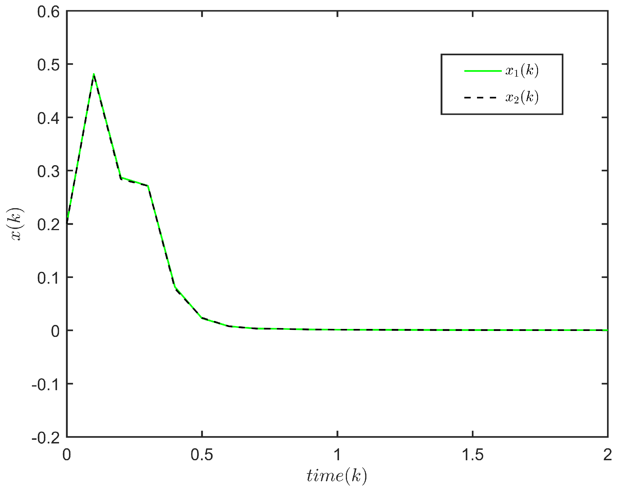
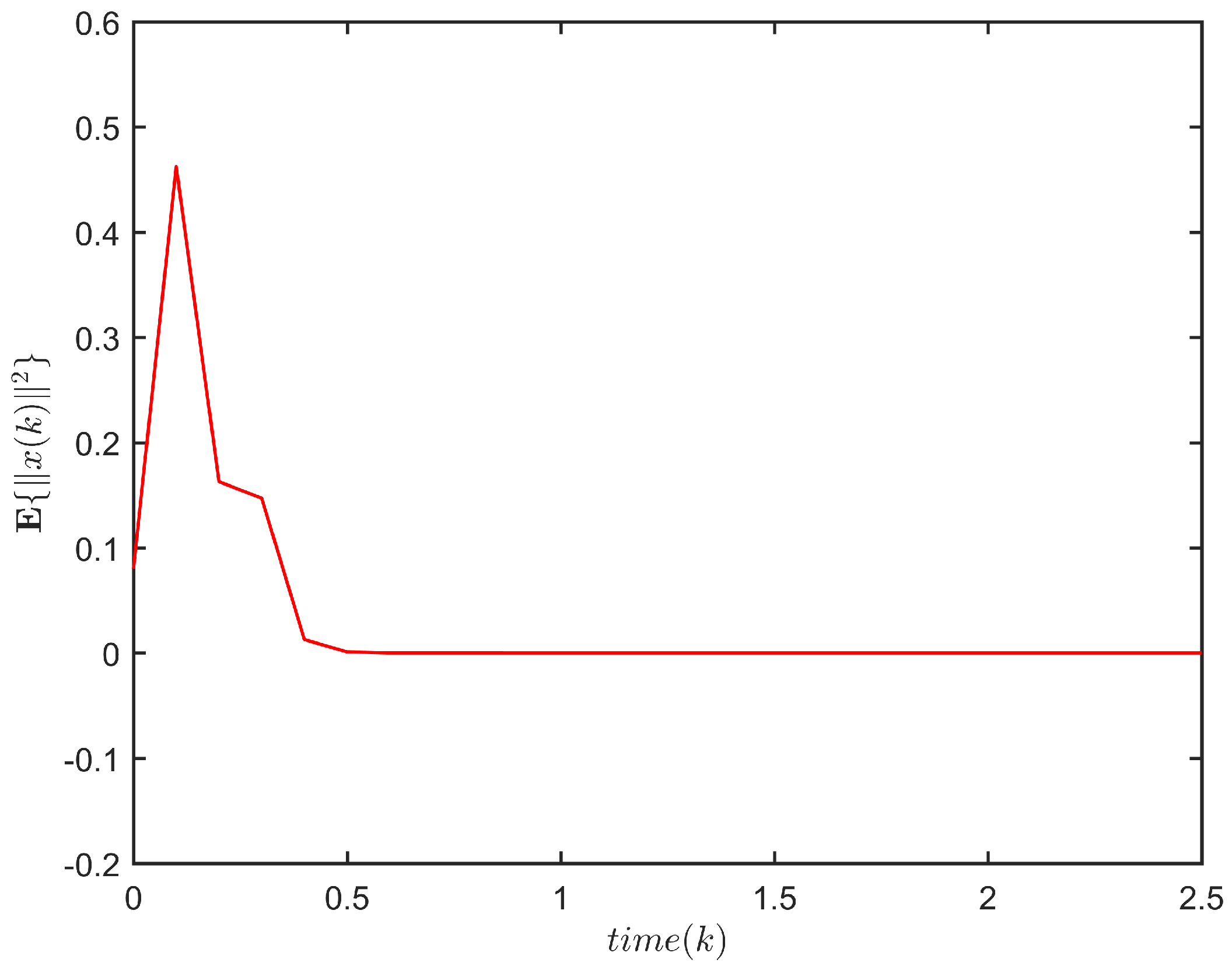
s u p l { 5 , 4 , , 1 } φ ( l ) 2 α = 3 ,
s u p l { 5 , 4 , , 1 } ( φ ( l + 1 ) φ ( l ) ) 2 δ = 0.2 .
The response of x ( k ) is plotted in Figure 1, and the evolution of E { x ( k ) 2 } is plotted in Figure 2. It is not difficult to see that E { x ( k ) 2 } 72.3245 , k N . This implies that system (1) is FTS subject to (3, 72.3245, 5).
In Table 1, we analyze the uncertain DSNS (1) with TVD. By Theorem 1, the minimum upper bound of β is obtained for α = 3 and N ( 10 , 20 , 40 ) .
Example 2.
Consider the uncertain DSNS (1)
M = 0.80 0.20 0.07 0.10 , M d = 0.01 0.01 0.02 0.01 , H = 0.01 0.05 0.02 0.01 , H d = 0.02 0.01 0.02 0.03 , F = 0.14 0.05 0.04 0.05 , F d = 0.02 0.20 0.10 0.05 , D = 0.01 0.07 0.01 0.01 , G = 0.01 0.00 0.01 0.05 , h m = 5 , h M = 20 , δ = 0.12 ,
and the following parameters μ = 0.68 , ϵ = 6 , ϵ d = 0.84 , λ 1 = 0.4123 , λ 2 = 0.4124 , λ 3 = 0.111 , λ 4 = 0.112 , λ 5 = 0.09 , λ 6 = 0.12 , λ 7 = 0.19 and λ 8 = 0.31 .
The response of x ( k ) is plotted in Figure 3, and the evolution of E { x ( k ) 2 } is plotted in Figure 4.
Moreover, let h ( k ) = 16 s i n ( k / 15 ) , k N , 5 h ( k ) 20 ,
φ ( l ) = 0.1 l + 0.2 0.1 l + 0.2 , l { 20 , 19 , , 0 } ,
satisfy the following conditions
s u p l { 20 , 19 , , 1 } E { φ ( l ) 2 } α = 2 ,
s u p l { 20 , 19 , , 1 } E { ( φ ( l + 1 ) φ ( l ) ) 2 } δ = 0.12 .
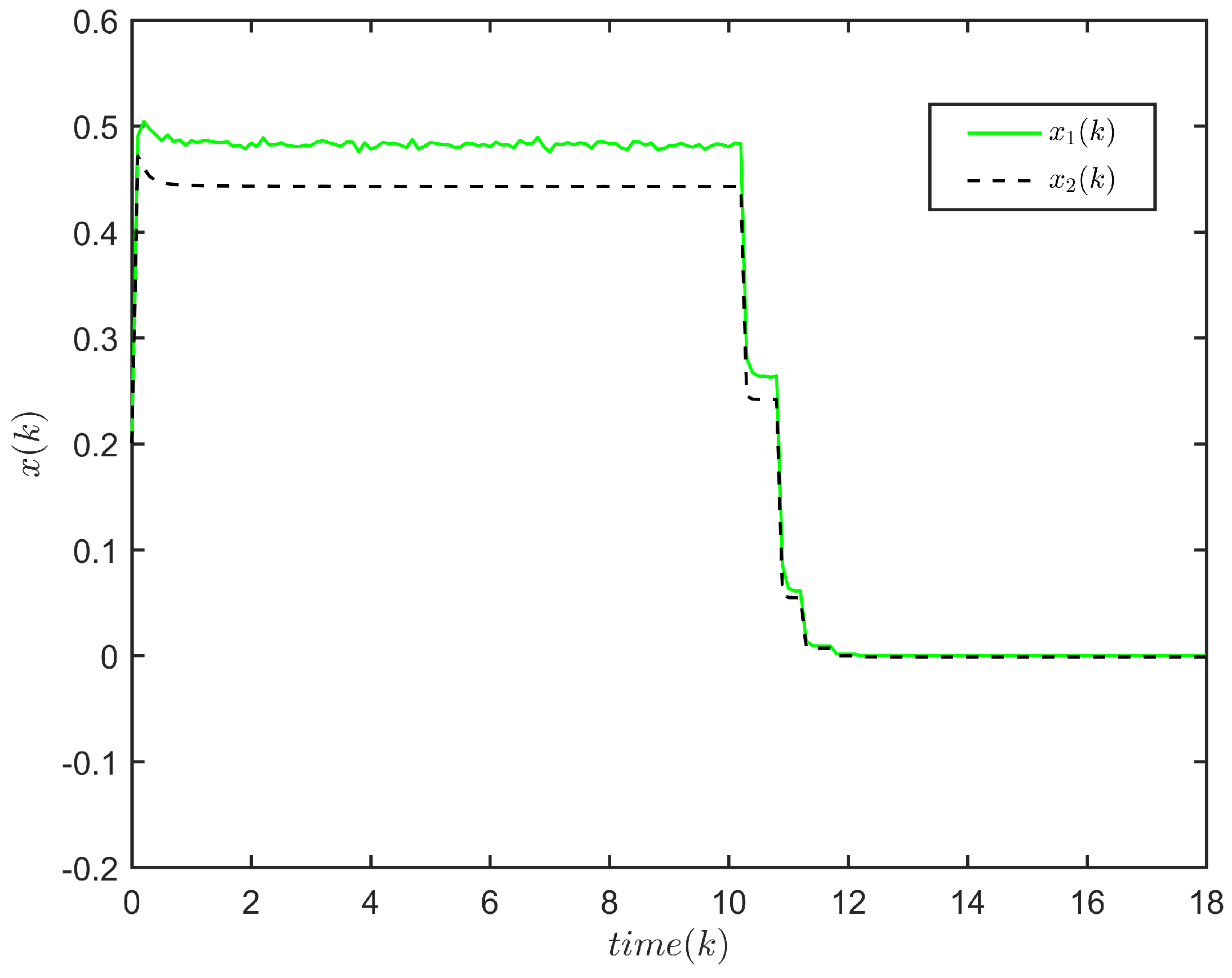
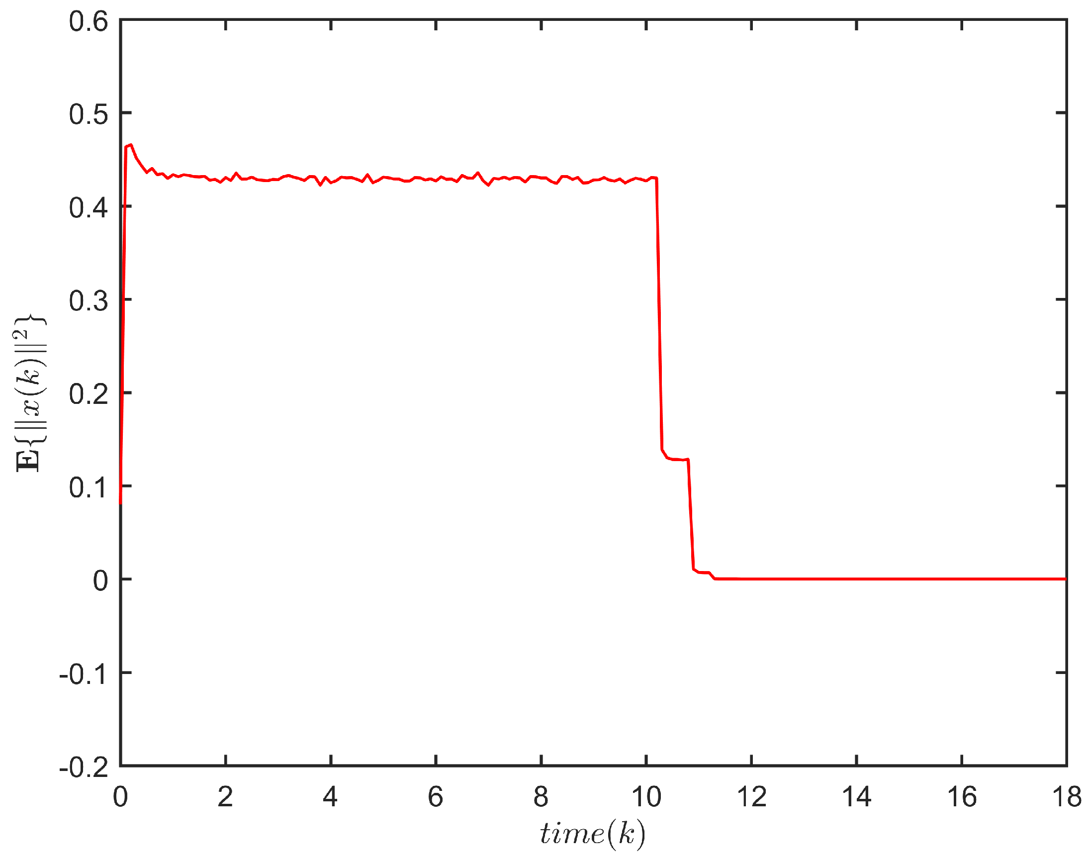
Figure 3 and Figure 4 depict the response of x ( k ) and the evolution of E { x ( k ) 2 } , respectively, for system (1). One has E { x ( k ) 2 } 41.7307 , k N . Thus, system (1) is FTS subject to (2, 41.7307, 5).
The minimum upper bound of the parameter β for system (2) is shown in Table 2, and the following conclusions are obtained:
(a)
The upper bound of the parameter β in this paper is smaller than that in the literature [41], which infers that the result in this paper is less conservative than that in [41].
(b)
The authors in [41] employed a novel approximation for a delayed state, which had a smaller approximation error compared with existing approaches. It is worth noting that the system in [41] did not consider the influence of external interference, uncertainty and nonlinear factors.
(c)
The authors in [13] adopted a new summation inequality called a discrete Wirtinger-based inequality. Although the results of [13] were better than that of this paper, the method adopted in [13] did not reflect random variables and uncertainty. Our results are more general.
The above two examples show that as the TVD increases, the longer it takes for the state response to reach stability. Therefore, the smaller the TVD is, the less conservative the FTS criterion is. It can also be seen that the stability of the state response is independent of the uncertain parameters and is related to nonlinear disturbances and TVD.

5. Conclusions

In this paper, we discussed the problem of FTS for uncertain DSNS with TVD. By constructing a new LKF with a power function ζ k j 1 and new summation inequalities, sufficient conditions to ensure the FTS and RAS of stochastic system were given. By using LMIs, less conservative stability criteria were established. For an uncertain DSNS with h ( k ) = h , this paper also provided the FTS criteria of the system. Finally, two simulation examples proved the validity of the method. It is noteworthy that the research method proposed can be applied to other systems, for instance, Markov jump systems, singular systems and discrete autonomous systems.

Author Contributions

Conceptualization, Y.L.; Data curation, W.L.; Funding acquisition, X.L.; Methodology, W.L.; Writing—original draft, J.W.; Writing—review and editing, X.L. and Y.L. All authors have read and agreed to the published version of the manuscript.

Funding

This work was supported by the National Natural Science Foundation of China (No. 61972236), Shandong Provincial Natural Science Foundation (No. ZR2018MF013).

Acknowledgments

The authors are grateful to the referees for their constructive suggestions.

Conflicts of Interest

The authors declare no conflict of interest.

References

  1. Aouiti, C.; Hui, Q.; Jallouli, H.; Moulay, E. Fixed-time stabilization of fuzzy neutral-type inertial neural networks with time-varying delay. Fuzzy Sets Syst. 2021, 411, 48–67. [Google Scholar] [CrossRef]
  2. Zhou, B.; Luo, W. Improved Razumikhin and Krasovskii stability criteria for time-varying stochastic time-delay systems. Automatica 2018, 89, 382–391. [Google Scholar] [CrossRef] [Green Version]
  3. Li, H.; Liu, Q.; Feng, G.; Zhang, X. Leader-follower consensus of nonlinear time-delay multiagent systems: A time-varying gain approach. Automatica 2021, 126, 109444. [Google Scholar] [CrossRef]
  4. Chen, L.; Bai, S.; Li, G.; Li, Z.; Xiao, Q.; Bai, L.; Li, C.; Xian, L.; Hu, Z.; Dai, G.; et al. Accuracy of real-time respiratory motion tracking and time delay of gating radiotherapy based on optical surface imaging technique. Radiat. Oncol. 2020, 15, 1–9. [Google Scholar] [CrossRef] [PubMed]
  5. Li, X.; Yang, X.; Song, S. Lyapunov conditions for finite-time stability of time-varying time-delay systems. Automatica 2019, 103, 135–140. [Google Scholar] [CrossRef]
  6. Zhang, C.K.; He, Y.; Jiang, L.; Wu, M.; Wang, Q.G. An extended reciprocally convex matrix inequality for stability analysis of systems with time-varying delay. Automatica 2017, 85, 481–485. [Google Scholar] [CrossRef]
  7. Zhou, B. Finite-time stability analysis and stabilization by bounded linear time-varying feedback. Automatica 2020, 121, 109191. [Google Scholar] [CrossRef]
  8. Li, R.; Zhao, P. Practical stability of time-varying positive systems with time delay. IET Control. Theory Appl. 2021, 15, 1082–1090. [Google Scholar] [CrossRef]
  9. Long, F.; Lin, W.J.; He, Y.; Jiang, L.; Wu, M. Stability analysis of linear systems with time-varying delay via a quadratic function negative-definiteness determination method. IET Control. Theory Appl. 2020, 14, 1478–1485. [Google Scholar] [CrossRef]
  10. Wu, B.; Wang, C.L.; Hu, Y.J.; Ma, X.L. Stability analysis for time-delay systems with nonlinear disturbances via new generalized integral inequalities. Int. J. Control. Autom. Syst. 2018, 16, 2772–2780. [Google Scholar] [CrossRef]
  11. Dong, Y.; Liang, S.; Wang, H. Robust stability and H control for nonlinear discrete-time switched systems with interval time-varying delay. Math. Methods Appl. Sci. 2019, 42, 1999–2015. [Google Scholar] [CrossRef]
  12. Ruan, Y.; Huang, T. Finite-Time control for nonlinear systems with time-varying delay and exogenous disturbance. Symmetry 2020, 12, 447. [Google Scholar] [CrossRef] [Green Version]
  13. Kang, W.; Zhong, S.; Shi, K.; Cheng, J. Finite-time stability for discrete-time system with time-varying delay and nonlinear perturbations. ISA Trans. 2016, 60, 67–73. [Google Scholar] [CrossRef] [PubMed]
  14. Stojanovic, S. Robust finite-time stability of discrete time systems with interval time-varying delay and nonlinear perturbations. J. Frankl. Inst. 2017, 354, 4549–4572. [Google Scholar] [CrossRef]
  15. Yang, X.; Li, X.; Cao, J. Robust finite-time stability of singular nonlinear systems with interval time-varying delay. J. Frankl. Inst. 2018, 355, 1241–1258. [Google Scholar] [CrossRef]
  16. Haddad, W.; Lee, J. Finite-time stability of discrete autonomous systems. Automatica 2020, 122, 109282. [Google Scholar] [CrossRef]
  17. Xi, Q.; Liang, Z.; Li, X. Uniform finite-time stability of nonlinear impulsive time-varying systems. Appl. Math. Model. 2021, 91, 913–922. [Google Scholar] [CrossRef]
  18. Alzabut, J.; Selvam, A.G.M.; El-Nabulsi, R.A.; Dhakshinamoorthy, V.; Samei, M.E. Asymptotic stability of nonlinear discrete fractional pantograph equations with non-local initial conditions. Symmetry 2021, 13, 473. [Google Scholar] [CrossRef]
  19. Rubbioni, P. Asymptotic stability of solutions for some classes of impulsive differential equations with distributed delay. Nonlinear Anal. Real World Appl. 2021, 61, 103324. [Google Scholar] [CrossRef]
  20. Dorato, P. Short time stability in linear time-varying systems. In Proceedings of the IRE International Convention Record Part 4, New York, NY, USA, 9 May 1961; Volume 4, pp. 83–87. [Google Scholar]
  21. Shi, C.; Vong, S. Finite-time stability for discrete-time systems with time-varying delay and nonlinear perturbations by weighted inequalities. J. Frankl. Inst. 2020, 357, 294–313. [Google Scholar] [CrossRef]
  22. Lin, X.; Liang, K.; Li, H.; Jiao, Y.; Nie, J. Finite-time stability and stabilization for continuous systems with additive time-varying delays. Circuits Syst. Signal Process. 2017, 36, 2971–2990. [Google Scholar] [CrossRef]
  23. Jia, R.; Wang, J.; Zhou, J. Fault diagnosis of industrial process based on the optimal parametric t-distributed stochastic neighbor embedding. Sci. China Inf. Sci. 2020, 64, 541–553. [Google Scholar] [CrossRef]
  24. Yu, X.; Yin, J.; Khoo, S. New Lyapunov conditions of stochastic finite-time stability and instability of nonlinear time-varying SDEs. Int. J. Control 2021, 94, 1674–1681. [Google Scholar] [CrossRef]
  25. Wang, M.; Liu, Y.; Cao, G.; Owens, D.H. Energy-based finite-time stabilization and H control of stochastic nonlinear systems. Int. J. Robust Nonlinear Control 2020, 30, 7169–7184. [Google Scholar] [CrossRef]
  26. Cheng, G.; Ju, Y.; Mu, X. Stochastic finite-time stability and stabilisation of semi-Markovian jump linear systems with generally uncertain transition rates. Int. J. Syst. Sci. 2021, 52, 185–195. [Google Scholar] [CrossRef]
  27. Yan, Z.; Song, Y.; Liu, X. Finite-time stability and stabilization for Itô-type stochastic Markovian jump systems with generally uncertain transition rates. Appl. Math. Comput. 2018, 321, 512–525. [Google Scholar] [CrossRef]
  28. Zhang, T.; Deng, F.; Zhang, W. Finite-time stability and stabilization of linear discrete time-varying stochastic systems. J. Frankl. Inst. 2019, 356, 1247–1267. [Google Scholar] [CrossRef] [Green Version]
  29. Liu, X.; Liu, Q.; Li, Y. Finite-time guaranteed cost control for uncertain mean-field stochastic systems. J. Frankl. Inst. 2020, 357, 2813–2829. [Google Scholar] [CrossRef]
  30. Niamsup, P.; Phat, V. Robust finite-time H control of linear time-varying delay systems with bounded control via Riccati equations. Int. J. Autom. Comput. 2018, 15, 355–363. [Google Scholar] [CrossRef]
  31. Wang, G.; Li, Z.; Zhang, Q.; Yang, C. Robust finite-time stability and stabilization of uncertain Markovian jump systems with time-varying delay. Appl. Math. Comput. 2017, 293, 377–393. [Google Scholar] [CrossRef]
  32. Liu, H.; Lin, X. Finite-time H control for a class of nonlinear system with time-varying delay. Neurocomputing 2015, 149, 1481–1489. [Google Scholar] [CrossRef]
  33. Zhou, M.; Fu, Y. Stability and stabilization for discrete-time Markovian jump stochastic systems with piecewise homogeneous transition probabilities. Int. J. Control. Autom. Syst. 2019, 17, 2165–2173. [Google Scholar] [CrossRef]
  34. Gao, M.; Zhao, J.; Sun, W. Stochastic H2/H control for discrete-time mean-field systems with Poisson jump. J. Frankl. Inst. 2021, 358, 2933–2947. [Google Scholar] [CrossRef]
  35. Rui, H.; Liu, J.; Qu, Y.; Cong, S.; Song, H. Global asymptotic stability analysis of discrete-time stochastic coupled systems with time-varying delay. Int. J. Control 2021, 94, 757–766. [Google Scholar] [CrossRef]
  36. Stojanovic, S. New results for finite-time stability of discrete-time linear systems with interval time-varying delay. Discret. Dyn. Nat. Soc. 2015, 2015, 480816. [Google Scholar] [CrossRef]
  37. Ouellette, D. Schur complements and statistics. Linear Algebra Its Appl. 1981, 36, 187–295. [Google Scholar] [CrossRef] [Green Version]
  38. Zuo, Z.; Li, H.; Wang, Y. New criterion for finite-time stability of linear discrete-time systems with time-varying delay. J. Frankl. Inst. 2013, 350, 2745–2756. [Google Scholar] [CrossRef]
  39. Seuret, A.; Gouaisbaut, F.; Fridman, E. Stability of discrete-time systems with time-varying delays via a novel summation inequality. IEEE Trans. Autom. Control 2015, 60, 2740–2745. [Google Scholar] [CrossRef] [Green Version]
  40. He, Y.; Wang, Q.; Xie, L.; Lin, C. Further improvement of free-weighting matrices technique for systems with time-varying delay. IEEE Trans. Autom. Control 2007, 52, 293–299. [Google Scholar] [CrossRef]
  41. Zhang, Z.; Zhang, Z.; Zhang, H.; Zheng, B.; Karimi, H.R. Finite-time stability analysis and stabilization for linear discrete-time system with time-varying delay. J. Frankl. Inst. 2014, 351, 3457–3476. [Google Scholar] [CrossRef]
Figure 1. The state response of system (1) ( 2 h ( k ) 5 ).
Entropy 24 00828 g001
Figure 2. The evolution of E { x ( k ) 2 } for (1).
Entropy 24 00828 g002
Figure 3. The state response of the system (1) ( 5 h ( k ) 20 ).
Entropy 24 00828 g003
Figure 4. The evolution of E { x ( k ) 2 } for system (1).
Entropy 24 00828 g004
Table 1. The minimum upper bound of the parameter β for system (1).
N102040
Theorem 3 [14]412 2.11 × 10 4 4.79 × 10 7
Theorem 1 200.4854 2.7723 × 10 3 7.0750 × 10 5
Table 2. The minimum upper bound of the parameter β for system (2).
N51020
Corollary 1 [13]81719
Theorem 1 [41]56125518
Corollary 1 28.1309 73.9878 424.0102
Publisher’s Note: MDPI stays neutral with regard to jurisdictional claims in published maps and institutional affiliations.

