
Effects of UAS Rotor Wash on Air Quality Measurements


U.S. Environmental Protection Agency, Office of Research and Development, Center for Environmental Measurement and Modeling, Raleigh, NC 27711, USA
*
Author to whom correspondence should be addressed.
Drones 2024, 8(3), 73; https://doi.org/10.3390/drones8030073
Submission received: 11 January 2024
/
Revised: 16 February 2024
/
Accepted: 18 February 2024
/
Published: 21 February 2024
(This article belongs to the Special Issue Drones for Wildfire and Prescribed Fire Science)
Abstract
:Laboratory and field tests examined the potential for unmanned aircraft system (UAS) rotor wash effects on gas and particle measurements from a biomass combustion source. Tests compared simultaneous placement of two sets of CO and CO2 gas sensors and PM2.5 instruments on a UAS body and on a vertical or horizontal extension arm beyond the rotors. For 1 Hz temporal concentration comparisons, correlations of body versus arm placement for the PM2.5 particle sensors yielded R2 = 0.85, and for both gas sensor pairs, exceeded an R2 of 0.90. Increasing the timestep to 10 s average concentrations throughout the burns improved the R2 value for the PM2.5 to 0.95 from 0.85. Finally, comparison of the whole-test average concentrations further increased the correlations between body- and arm-mounted sensors, exceeding an R2 of 0.98 for both gases and particle measurements. Evaluation of PM2.5 emission factors with single-factor ANOVA analyses showed no significant differences between the values derived from the arm, either vertical or horizontal, and those from the body. These results suggest that rotor wash effects on body- and arm-mounted sensors are minimal in scenarios where short-duration, time-averaged concentrations are used to calculate emission factors and whole-area flux values.
1. Introduction
The growing technical capability in both multicopter unmanned aircraft systems (UASs) and sensors for gas and particle concentrations has presented new opportunities for their use in measuring air pollution [1,2,3]. The three-dimensional, positional freedom of UASs and their ability to maneuver or hold position offer significant advantages over other ground measurement methods and manned aircraft in specific measurement cases. Remotely piloted UASs allow measurements without risk to personnel and, for situations like fires, without exposing measurement equipment to hazards. While a primary constraint of using UASs for air measurements can be the payload capacity [4], the advent of lightweight sensors and computers has significantly ameliorated this concern. Consequently, UAS applications for air measurements are rapidly being presented in the literature [4,5].
An oft-cited concern for use of multicopter UASs in making air quality measurements is the potential effect of the rotor downwash on the sensor readings and sampling system [4]. Rotor downwash has been visually demonstrated by Crazzolara et al. [6] and has been the subject of numerous computational studies [7,8,9,10,11], as cited in Burgués and Marco [4]. While air disturbances are generally considered to be limited above the rotors (~50 cm above the UAS, [12]), alongside the UAS (see references in Burgués and Marco [4]), and especially in front of a moving UAS, they can extend multiple UAS diameters below the rotors [13].
Numerous authors mention the deleterious effects of rotor downwash on air quality sensor accuracy and time-responsiveness. For spatial- and temporal-specific concentration measurements, Neumann et al. [14] indicate that the rotor wash can dilute the concentration of a target gas depending on the position and method of sampling. Gas concentrations measured passively by a sensor mounted on the body, when pressure-aided by rotor wash and a sampling tube, and with a sampling tube beyond the radius of the UAS, resulted in increased concentrations in that order, but none reached the level of the reference gas concentration. Similar concerns prompted Burgués et al. [13] to employ 10 m long sampling tubes dangling from the UAS to reach beyond the rotor wash effects in measuring concentrations close to the source. Li et al. [15] were motivated to study the position of UAS-mounted intake ports on gas and particulate matter concentrations due to stated considerations of rotor air flow disturbances. Burgués et al. [13] indicated that intense downwash from the rotors “strongly distorts” the gas distribution, leading to sensor errors. This is particularly noted for sensing applications in which the UASs fly close to point or surface emitters. Nonetheless, Gullett et al. [16] found that body-mounted gas sensors on a UAS determined plume-averaged gas emission factors from a natural gas boiler within 4–6% of the stack sample emission rate, and Arroyo et al. [17], in comparing stationary versus UAS gas measurements, achieved an R2 of 0.67 and 0.68 for NO and NO2, respectively, with a horizontal sampling tube extended only a few centimeters beyond the propeller radius.
Methods have been employed to avoid the rotor wash phenomena demonstrated by Crazzolara et al. [6] on smoke plumes, including both horizontal and vertical arms extending from the body of the UAS. Computational fluid dynamics calculations [18] as well as observations confirm that the rotor wash envelope is greater below the rotors than above, hence favoring placement of sensors and sampling inlets above the UAS. Prior to measuring near roadway air pollution, Samad et al. [19] used smoke tracer experiments to demonstrate practically negligible effects of rotor wash when their sensor was positioned vertically 90 cm above their hexacopter body. Maintenance of flight velocities with sensors mounted on the leading, horizontal arm have also been thought to avoid the rotor wash “envelope” around the UAS body. Use of a horizontal extension arm for sampling elevated and channeled sources, such as chimneys and flares, was advocated by Burgués and Marco [4], but for diffusive area sources, the authors argued that the UAS would have to fly close to the ground for near-source sampling, leading to aircraft risks and strong dilution of the emissions. Others have developed mathematical corrections for rotor wash effects on stationary UAS particulate matter measurements by comparing both pole-mounted and UAS-based measurements [20].
The placement of sensors or sampling inlets on rotorcraft has been studied in detail. Roldán et al. [21] studied placement of sensors on a UAS due to stated effects of rotor air flow on gas concentration measurements. Their experiments with and without rotor movement found less than a 4% difference in the gas measurement, a difference which the authors stated may also be attributable to variables other than rotor wash. Likewise, Greene et al. [22] conducted experiments and determined that sensors should be placed one-quarter length of the propeller from the tip to minimize influences of turbulence and frictional heating while still maintaining adequate airflow.
While visual and computational studies have investigated rotor wash, scant comparative testing information is available documenting potential effects on gas and particle measurements, particularly the latter, leaving persistent questions about the need for compensatory measures, such as use of sensor-mounted extension arms. Similarly, when the sampling objective is related to area flux calculations or emission factors based on ratios of measured components, published evidence for rotor wash effects is lacking. This work employed a series of laboratory and field tests to compare simultaneous gas and particle measurements from identical sensor sets to assess the potential effects of rotor wash on air quality measurements.
2. Materials and Methods
2.1. Emission Sampling
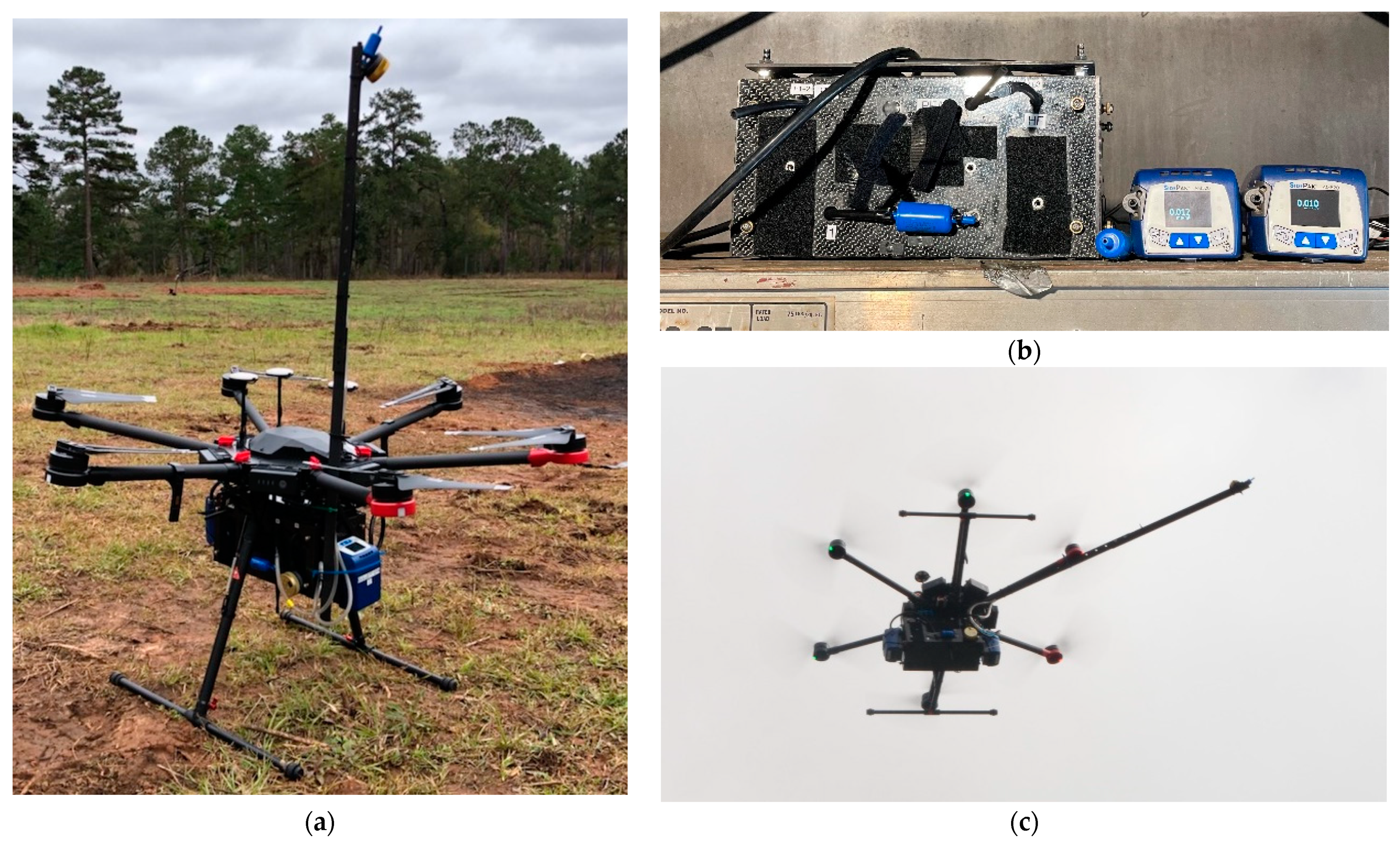
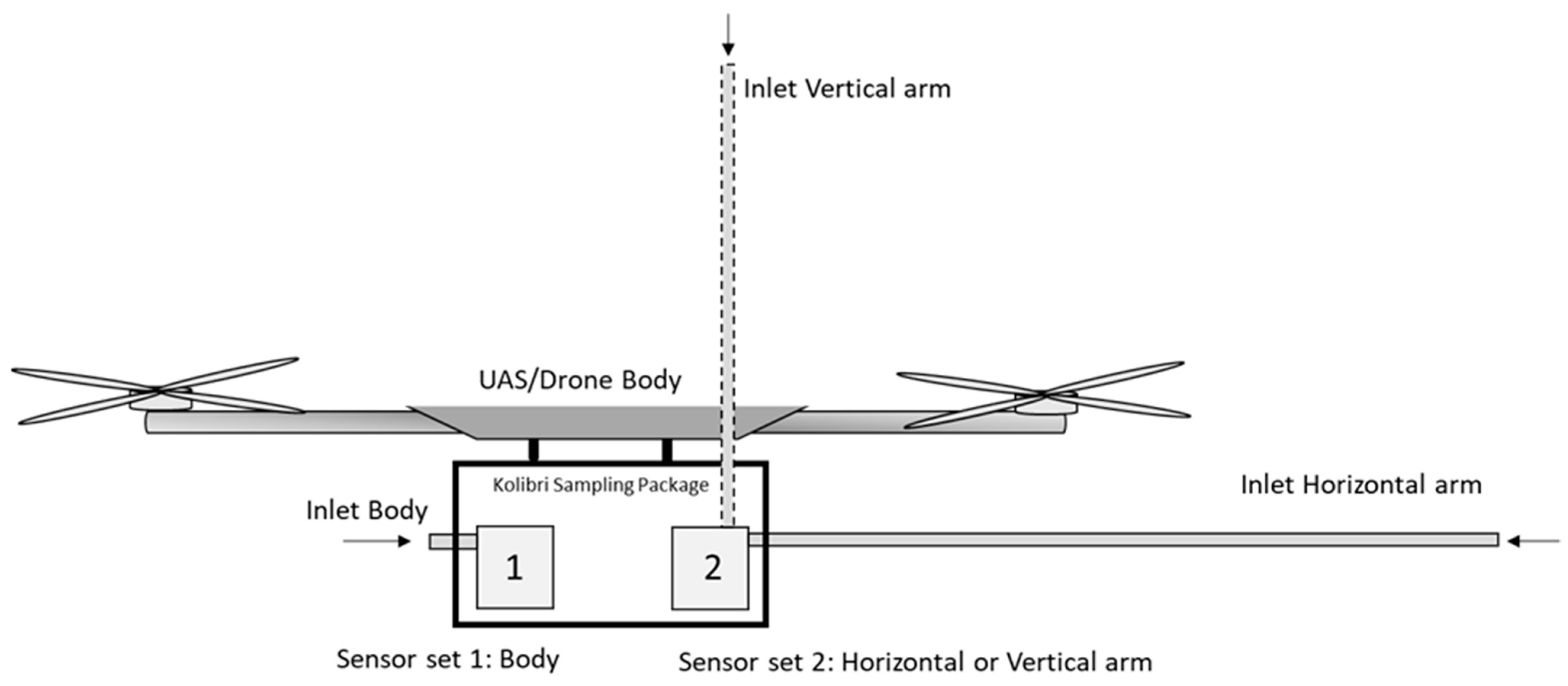
The measurements were conducted using a ~4 kg instrument package called the Kolibri, which was configured with two sampling sets, each consisting of carbon dioxide (CO2) and carbon monoxide (CO) sensors, batch particulate matter impactors < 2.5 microns in diameter (PM2.5(b)), and time-resolved PM2.5(t) instruments. Both sampling sets were employed simultaneously, one mounted on a sampling arm and the other mounted on the UAS body. A 6-rotor (hexacopter) UAS (DJI Matrice M600) was used as the sampling platform. The Kolibri package was attached directly underneath the body of the UAS (Figure 1a,b). One measurement set (PM2.5(b) impactor, CO2 and CO inlet filter, and PM2.5(t) inlet tube) was fixed to the body of the Kolibri. Simultaneously, a 1.10 m arm with a 1.37 m long sampling tube was attached either horizontally or vertically to the UAS body (Figure 1a,b and Figure 2) for comparison with the body-fixed sampling set. The horizontal arm was secured underneath one of the propeller arms, extending 42 cm (>1 propeller length) from the propeller blade tip. The second measurement set (PM2.5(b) impactor, CO2 and CO inlet filter, and PM2.5(t) inlet tube) was attached at the tip of the arm connected to their respective instrument/pumps in or on the Kolibri using 1.37 m long antistatic polyurethane tubes (Figure 2). The vertical arm extended 0.75 m above the center of the UAS body.
To assess any dissimilarities between the time-resolved instruments, the two sets of CO2 and CO sensors were first evaluated in an indoor laboratory setting using CO and CO2 calibration gases with a split inlet (“Y”). These two sets of sensors and the PM2.5(t) instruments were further tested side-by-side in a controlled laboratory setting using the US EPA’s open burn test facility (OBTF) in NC, US (described more fully elsewhere [23,24]). Six tests were conducted: three with 1.37 m long antistatic polyurethane tubes for sampling and three without (Figure 1c) to understand potential effects of the inlet tube lengths. The mass of burned biomass (a mix of pine needles and oak leaves) varied from 0.25 to 0.5 kg.
Tests were also conducted in the field at Tall Timbers Research Station, Florida, US. Four 10 by 10 m square plots were hand-covered with a layer of longleaf pine straw (Pinus palustris) as the fuel source. A total of eleven burn tests were conducted over four days, with five burns conducted simultaneously sampling with one set of sensors sampling directly under the UAS body and the second set of sensors sampling connected to the horizontal arm, and six burns simultaneously sampling with one set of sensors sampling directly under the UAS body and the second set of sensors sampling connected to the vertical arm (Figure 2). The UAS was positioned within the plume of these small burn plots and remained relatively stationary.
2.2. Emission Sampler
The Kolibri system includes a microcontroller that allows the PM2.5(b) and sensor pumps to be remotely controlled and for the operator to view CO2 and CO concentrations in real time. Measured parameters and instruments are shown in Table 1. The CO2 and CO concentrations were measured using a K30 FR (SenseAir, Delsbo, Sweden) nondispersive infrared (NDIR) sensor and an e2V EC4-500-CO electrochemical sensor (SGX Sensortech, Essex, UK), respectively. A micropump with a flow rate of 1 L/min (C120CNSN30, Sensidyne, St. Petersburg, FL, USA) was used to draw in the plume gases through a particulate gas filter (Balston 9922-05-DQ) before reaching the CO2 and CO sensors. The CO2 and CO detection ranges were 0–10,000 ppm and 1–300 ppm with a resolution of 1 ppm, respectively. A full description of the Kolibri and further details on the CO2 and CO sensors has been described elsewhere [16,25,26]. Due to microcontroller board limitations, the two CO2 sensor signals were read differently: one was digital (sensor set 1 used for the body measurements) and one was analog (sensor set 2 used for the arm measurements). The CO2 and CO sensors were calibrated before the tests and checked for drift afterwards using calibration gases traceable to the National Institute of Standards and Technology (NIST) standards following steps as described in OTM-48 [27].
Batch PM2.5(b) samples were collected to determine photometric calibration factors (PCFs) for calibrating the real-time PM2.5(t) samplers for the optical properties of the source particles. Personal Modular Impactors (SKC Inc., Eighty Four, PA, USA) used 37 mm Teflon filters with a pore size of 2.0 µm and a constant microair pump at 3.0 L/min (C120CNSN60, Sensidyne, St. Petersburg, FL, USA). Pump flow rates were calibrated before the tests using a Go-Cal flow meter (Sensidyne, St. Petersburg, FL, USA). The filters were pre- and postweighed following the procedures in OTM-48 [27]. Two SidePaksTM AM520 (TSI, Shoreview, MN, USA) were used to measure time-resolved PM2.5(t) concentrations. The SidePaks measure particles using a light-scattering diode laser with concentrations ranging from 0.001 to 100 mg/m3. The SidePaks were zeroed by attaching a filter to the inlet and the flow rate was calibrated to 1.7 L/min using a 0.01–20 L/min Go-Cal flow meter (Sensidyne, St. Petersburg, FL, USA) before the tests. All data were logged at 1 Hz.
2.3. Calculations
Emission factors from open biomass fires were calculated using the carbon mass balance approach as described in OTM-48 [27]. This method relates the carbon fraction in the fuel (approximate 0.5 for biomass) to the carbon mass sampled from the CO2 and CO in the plume, allowing determination of an emission factor expressed as mass of pollutant per mass of biomass combusted (e.g., g PM2.5/kg biomass burned). The modified combustion efficiency (MCE) was calculated as ∆CO2/(∆CO2 + ∆CO), which was used as a measure of how well the biomass was combusted during the burns.
The time-resolved, optical SidePak PM2.5(t) instrument requires calibration to an integrated filter mass, as the measurements depend on the optical characteristics of the particles in question. A PM2.5(b) batch filter was sampled simultaneously with the optical measurements for all field burns, resulting in an average PCF of 2.6, which was applied to all optical PM data.
To determine any differences in concentration and emission factors between the sensors themselves and sensor locations (body and arm), single-factor one-way analysis of variance (ANOVA) was used with a level of significance α = 0.05. The significance value (ANOVA-returned p value) has to be less than α = 0.05 and the measure of the variance ratio between two populations (F/Fcrit value) has to be greater than 1.0 to demonstrate significant difference [28]. Correlation plots were used to observe the relationship between data derived from the sensors themselves and their locations (body and arm), and the coefficient of determination, R2, was used to indicate how well the derived data fit the linear curve. The root mean squared error (RMSE) was derived to measure the error between two pair of sensors and sensor locations (body and arm).
3. Results
3.1. Indoor Laboratory Instrument Comparison
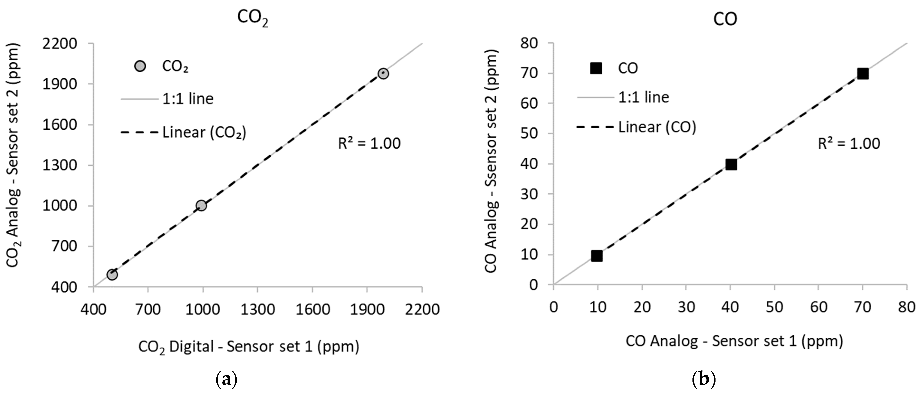
Prior to field sampling, tests were conducted in the laboratory to (a) compare the two paired sets of sensors under a controlled environment and (b) understand whether the identical CO2 sensors, one reporting with analog signals and the other with digital signals, produced similar results. The identical two CO2 sensors showed a difference of less than 2% in concentration when fed with a constant flow of 500, 1000, and 2000 ppm CO2 calibration gas. The CO sensors (both analog) showed a less than 1% difference when fed with a constant flow of CO calibration gas at 10, 40, and 70 ppm. Figure 3 shows the measured values from the two CO2 and the two CO sensors plotted against each other, which showed excellent correlation (R2 = 1.0, p < 0.02) and RMSEs of 11.6 and 0.09 ppm for CO2 and CO, respectively. For steady gas concentrations as supplied by the calibration gas standards, little impactful difference was observed in the sensor outputs.
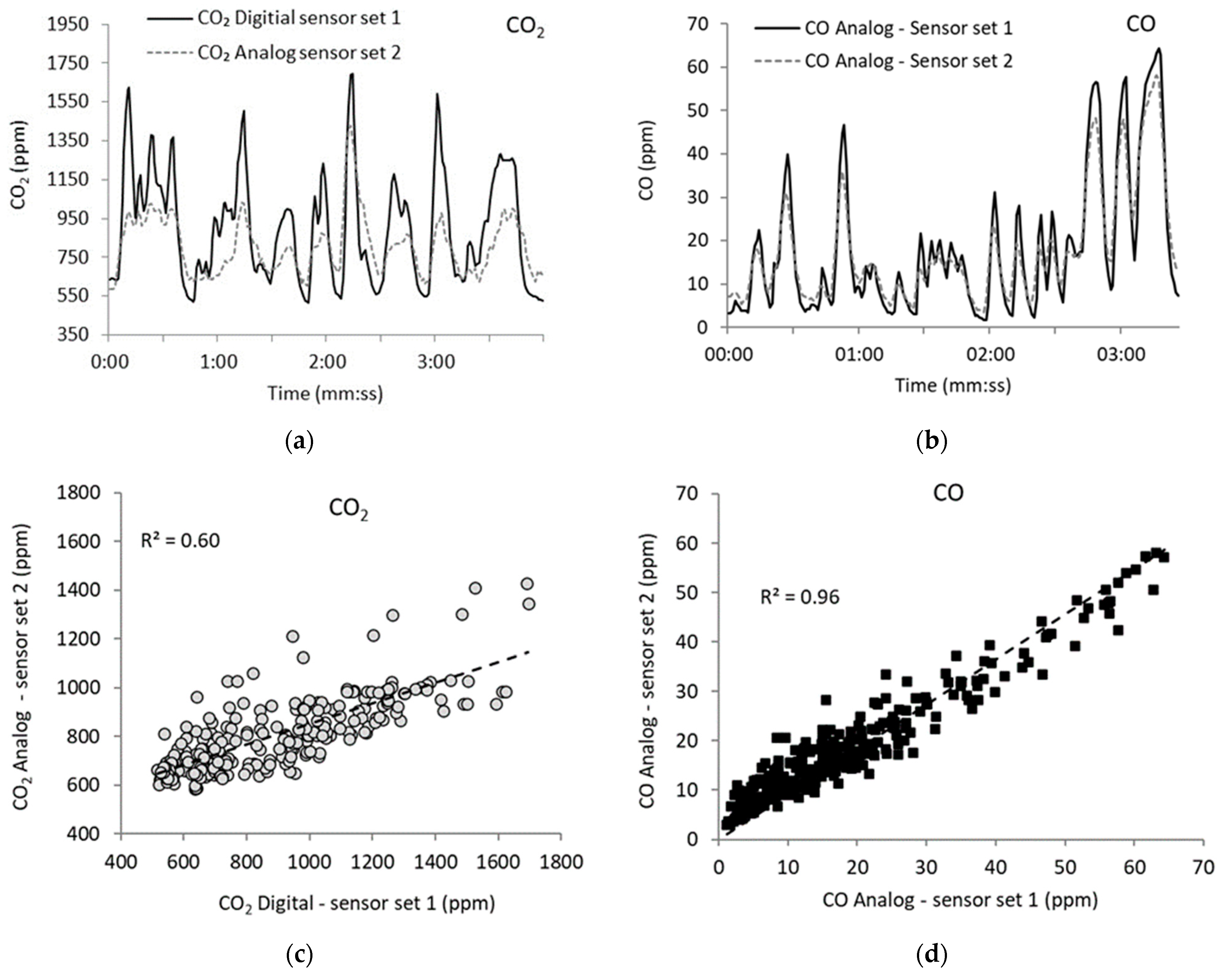
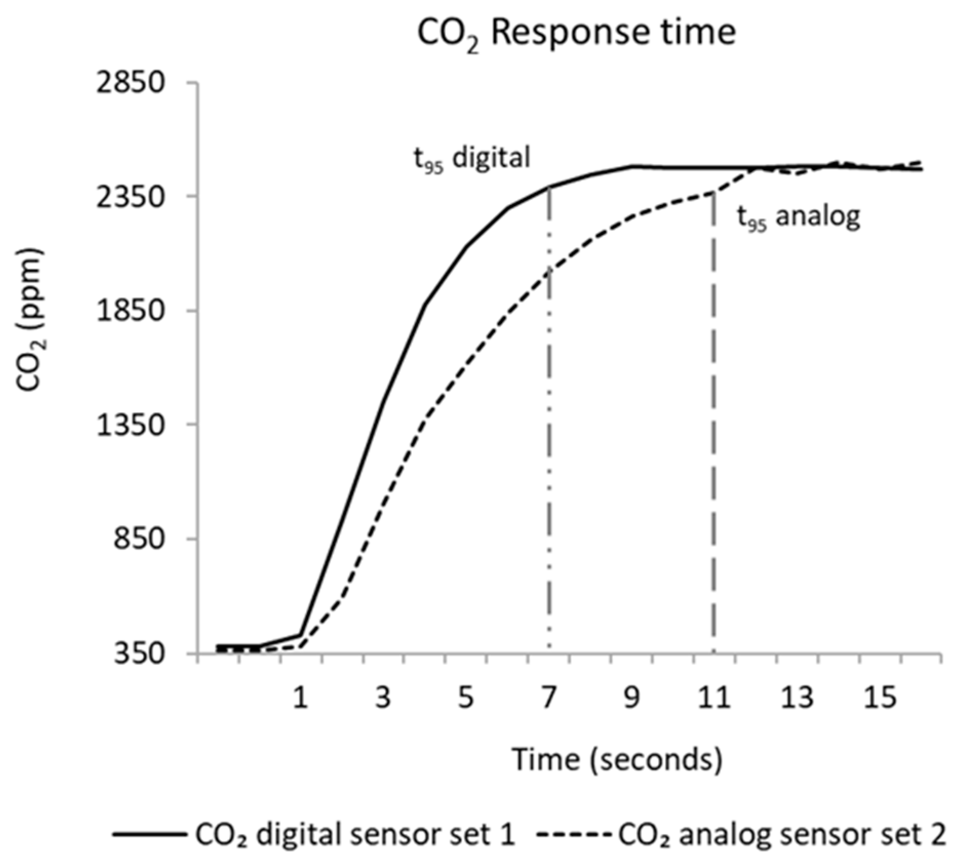
The two pairs of gas sensors were also introduced to quick fluctuations of CO2 and CO calibration gas through a Y inlet to simulate situations in which small, discrete plumes rapidly mix and exchange with ambient air. A tube supplying calibration gas was moved back and forth (~1 Hz) past the Y inlet leading to the two sensors. The results are shown in Figure 4a,b, indicating lower concentration values from the analog CO2 sensor (807 ppm average) than the digital sensor (average 898 ppm), an 11% difference, and a low correlation, with an R2 = 0.60 (p < 0.02) and with an RMSE of 210 ppm (Figure 4c). These results indicate the difference in performance between the analog CO2 channel and the digital channel under conditions of rapidly fluctuating concentrations in contrast to results observed under steady-state conditions (Figure 3). These differences in the CO2 sensor readings are related to the slower response time and greater noise of the analog output as compared to the digital output, as observed in the sensors’ response to a step change in the concentration (Figure 5), and resulting in the lack of a 1:1 slope, as shown in Figure 4c. Figure 5 shows that the analog sensor response time to reach 95% of the input gas concentration (t95) is 11 s, while the digital sensor is 4 seconds faster, t95 = 7 s.
The two CO traces under fluctuating gas exposure showed similar concentration trends (R2 = 0.96 and p < 0.003, Figure 4d) and both resulted in the same average concentration of 18 ppm and an RMSE of 4.4 ppm. These results allowed subsequent comparisons to be made with confidence, knowing that the identical sensors (both analog) performed equally.
3.2. Open Burn Test Facility Testing
Combustion tests of the paired gas sensors were undertaken in the OBTF, a well-mixed chamber (70 m3) with a 1 m2 burn pan loaded with longleaf pine needles. Six burns were conducted, the first three comparing the two sets of sensors side-by-side (two CO, two CO2, and two PM2.5(t)) and the second three comparing the effect of adding a 1.37 m sampling tube before sampling sensor set #2 (one CO, one CO2, and one PM2.5(t)). The addition of the tube was meant to simulate the effect of adding a sampling-arm-mounted sensor, albeit without the rotor wash. For the CO2 sensors, the analog sensor (sensor set #2) was always placed on the sampling arm and the digital CO2 sensor (sensor set #1) on the UAS body.
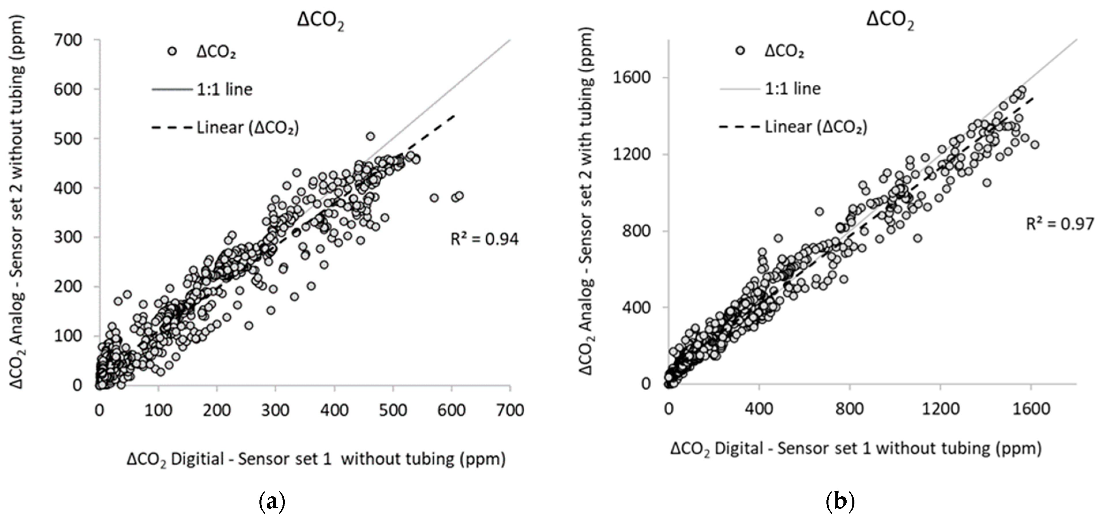
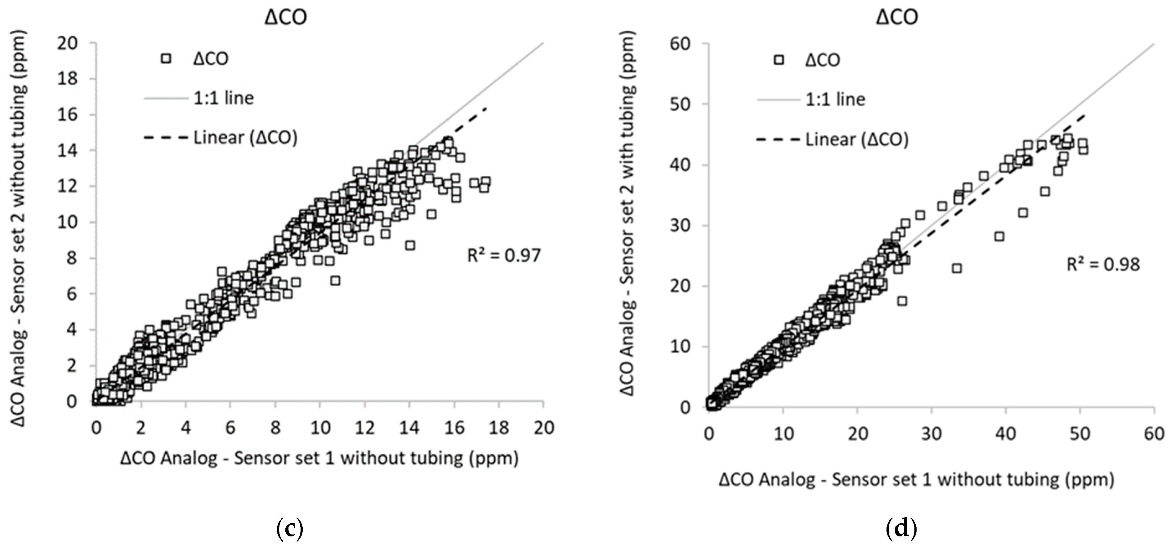
No statistically significant differences in the average CO2 and CO concentrations were found between the sensors when using the 1.37 m long sampling tube simulating the arm measurements compared to the body-mounted simulation without the sampling tube (CO2 body 873 ± 133 ppm, CO2 arm 892 ± 146 ppm: p = 0.88, F/Fcrit 0.003; CO body 12 ± 4.2 ppm, CO arm 12 ± 4.2 ppm: p = 0.96, F/Fcrit 0.0002). The two CO2 and two CO sensors, with or without the 1.37 m long tubing, showed great intracorrelation, as displayed by their R2 values from 0.94 to 0.98 (p < 0.001), respectively (Figure 6a–c). The RMSE for all burns was 58 and 1.1 ppm for CO2 and CO, respectively. The considerably better correlation and RMSE found for the CO2 sensors in the OBTF test compared to the laboratory test is likely due to the lack of fast fluctuations in the OBTF concentrations, as the smoke mixing results in more homogeneity in concentration prior to reaching the sensor inlets. The difference in the t95 values for the analog and digital CO2 sensors (4 s) and the increased residence time in the sampling tube (1.7 s) resulted in no statistical effect on the concentrations under these test conditions.
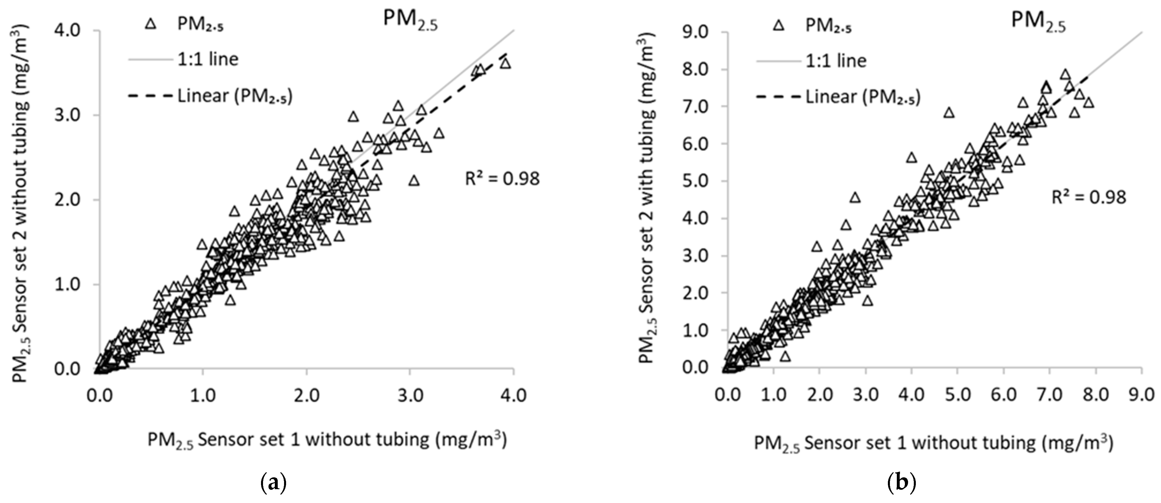
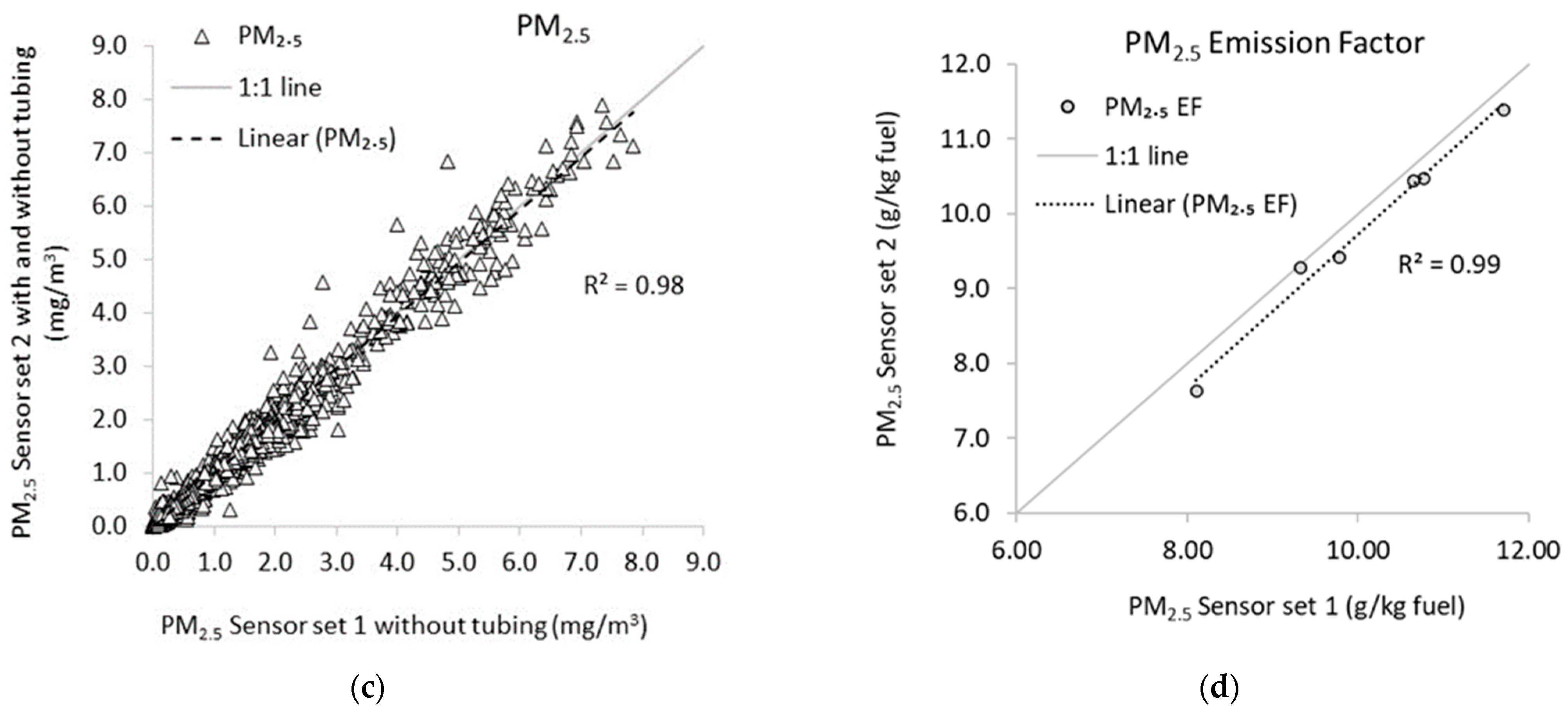
Simultaneously with the gas-phase tests, the SidePak particle instruments were compared in the OBTF. Figure 7a–c show excellent correlation (R2 = 0.98, p < 0.0001) between the two side-by-side PM2.5 instruments’ concentrations, both without sampling tubes (Figure 7a, p < 0.001 and RMSE 0.12 mg/m3), and when the inlet to one instrument used the 1.37 m sampling tube (Figure 7b, p < 0.001 and RMSE 0.24 mg/m3), simulating the use of the arm on the UAS. No significant difference was found between either configuration (PM2.5 body 5.5 ± 1.4 mg/m3, PM2.5 arm 5.5 ± 1.5 mg/m3: p = 0.7, F/Fcrit = 0.04). Likewise, the PM2.5 emission factors (Figure 7d, R2 0.99 and p < 0.001) showed no significant difference between the instrument/sensors used for the body simulation and the arm simulation (with tubing): PM2.5 body 10.1 ± 1.3 g/kg fuel versus PM2.5 arm 9.8 ± 1.3 g/kg fuel (p = 0.7, F/Fcrit = 0.03, RMSE 0.32 g/kg fuel) with nearly identical MCEs of 0.969 ± 0.004 and 0.970 ± 0.004, respectively.
3.3. Field Tests of Rotor Wash Effects
The two instrument sets were affixed to a multicopter UAS to measure CO2, CO, and PM2.5 concentrations from the body and horizontal arm during five burns of longleaf pine needle burns and another six burns with the sensors affixed to the body and vertical arm. Single-factor ANOVA tests for each pollutant were conducted, comparing the body and horizontal arm measurements (five burns), and body and vertical arm measurements (six burns).
3.3.1. CO2 and CO
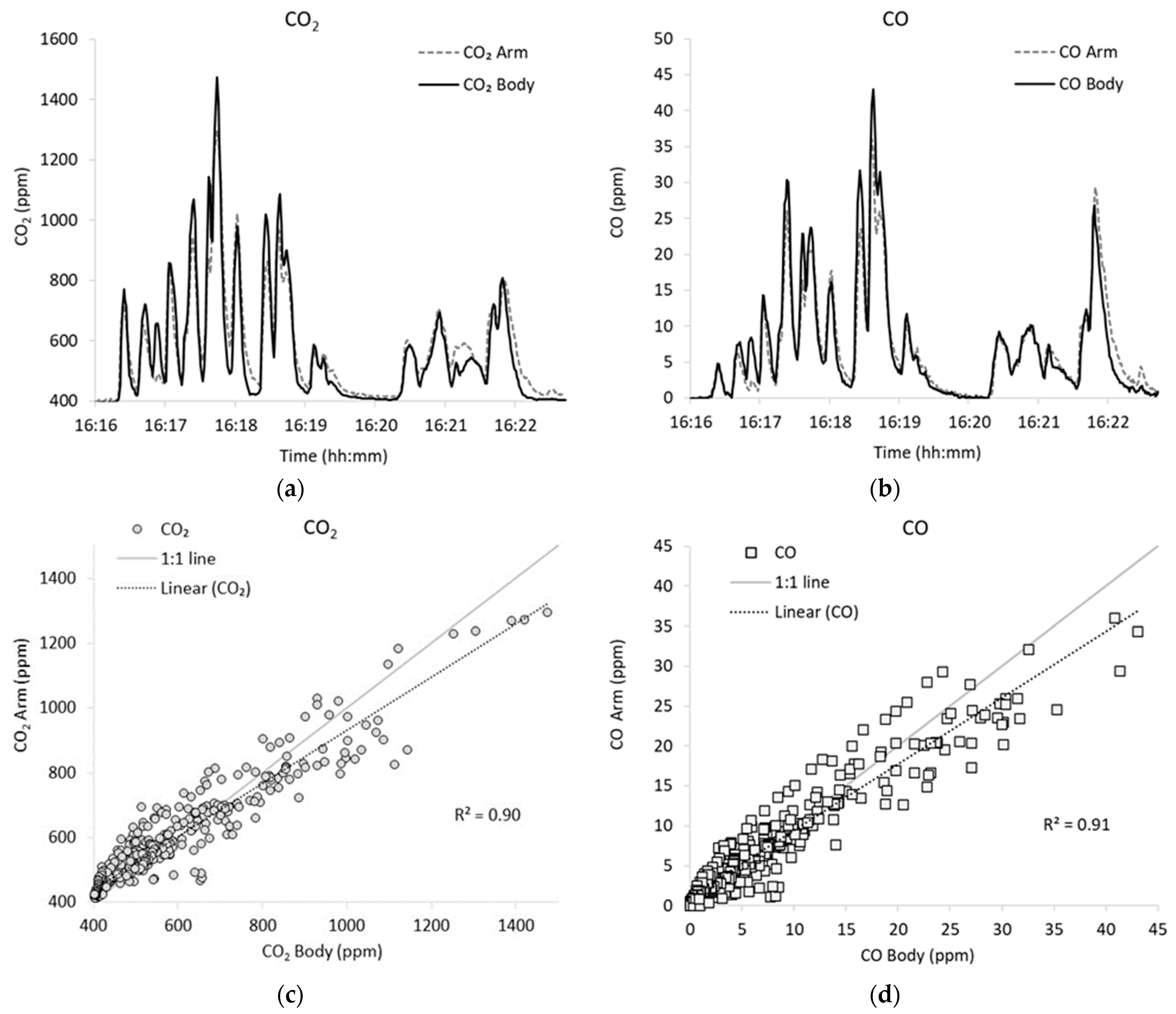
Figure 8a,b show an example of typical time-resolved concentration traces (CO2 and CO, respectively) from one of the representative burns for the two pairs of sensors, one pair mounted vertically on an arm and one pair on the body. The time-resolved data showed only minor dissimilarities between either of the two sensor pairs, supported by a typical correlation plot, shown in Figure 8c (CO2, R2 = 0.90, p < 0.001, RMSE = 63 ppm) and Figure 8d (CO, R2 = 0.91, p < 0.001, RMSE = 2.5 ppm), for one burn.
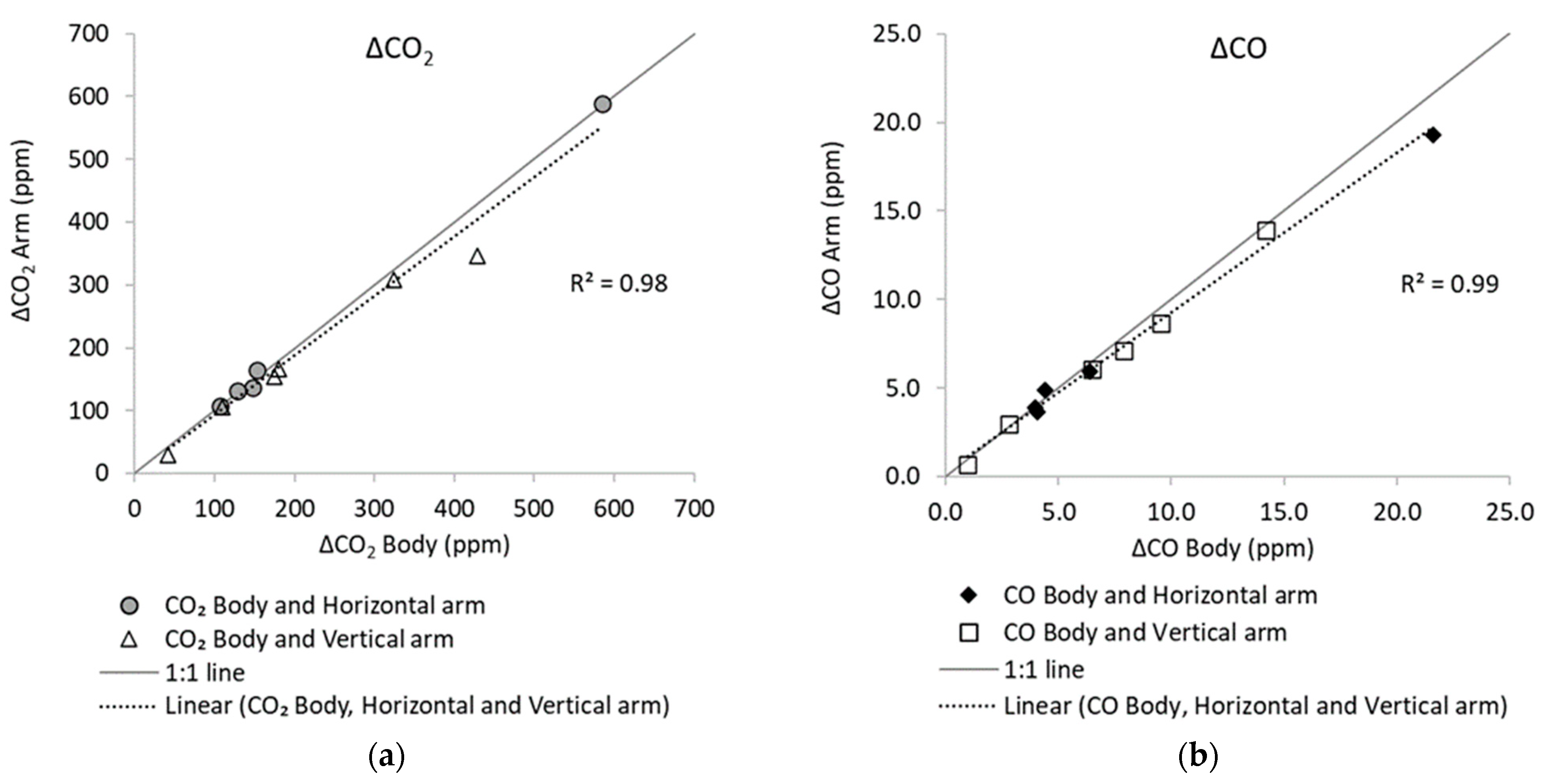
The average 1 Hz CO2 and CO concentrations were calculated from each burn and sensor, and plotted against each other, as shown in Figure 9a,b. Both pairs of sensors showed better correlation using burn-average data (CO2 R2 = 0.98, p < 0.001, RMSE = 27 ppm; CO R2 = 0.99, p < 0.001, RMSE = 0.84 ppm) than time-resolved data, consistent with the OBTF data. The overall CO2 average from all burns was 217 ± 163 ppm and 204 ± 156 ppm for the body-mounted and arm-mounted sensors, respectively, while the respective CO values were 7 ± 6 ppm and 7 ± 5 ppm. No significant difference was found when comparing the whole-burn average concentration between the body- and arm-mounted measurements for either the CO2 or CO sensors (CO2: p = 0.9, F/Fcrit = 0.01; CO p = 0.8, F/Fcrit = 0.01). Furthermore, no difference was found in measuring the CO2 or CO using a horizontal or vertical arm compared to the body measurement (body vs. horizontal arm CO2 p = 0.99, F/Fcrit = 0.00002; CO p = 0.91, F/Fcrit = 0.003; body vs. vertical arm CO2 p = 0.75, F/Fcrit = 0.02; CO p = 0.88, F/Fcrit = 0.005).
3.3.2. PM2.5
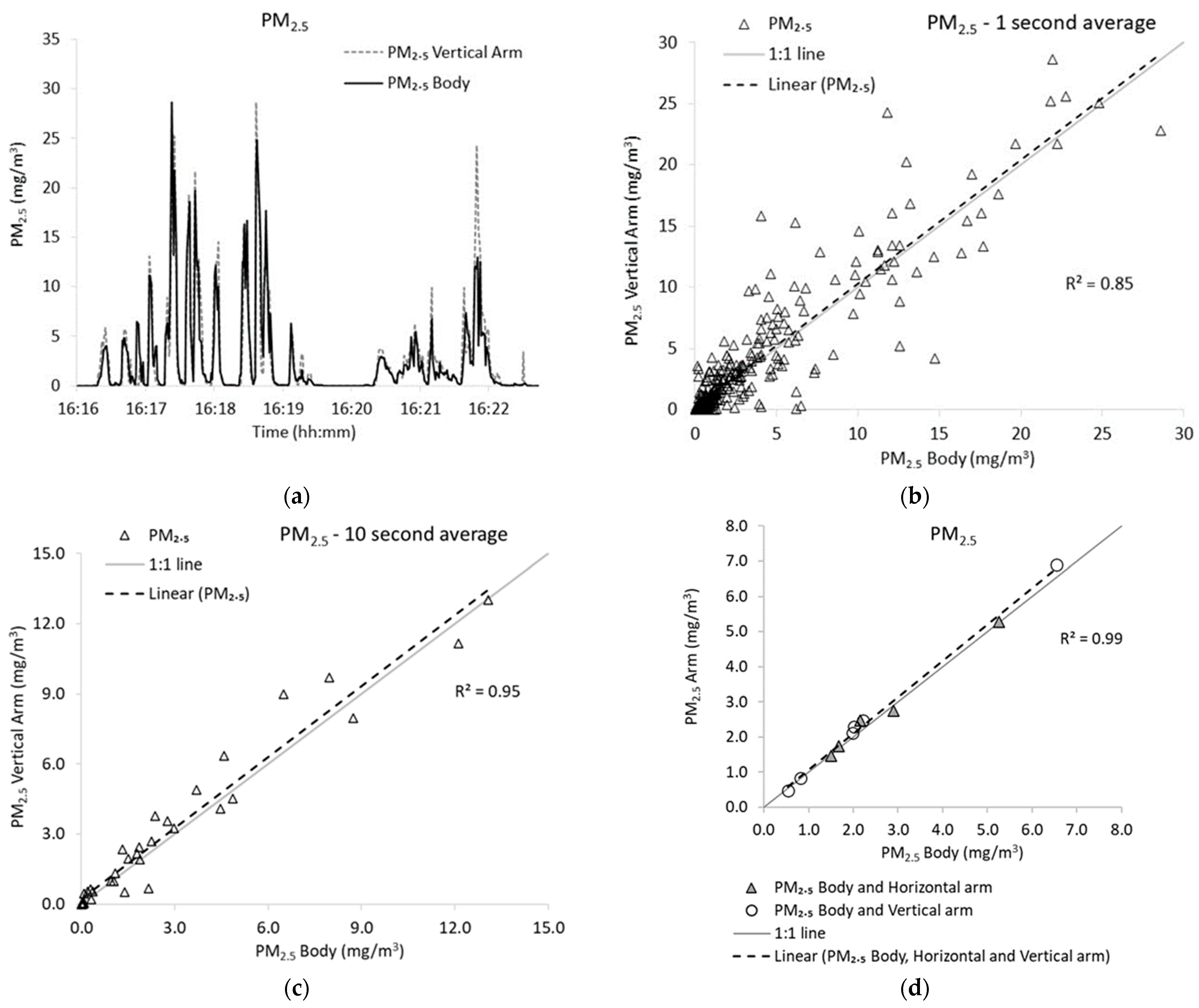
Figure 10a exhibits traces of the time-resolved (1 s data) PM2.5 concentration from a typical field burn, showing minor dissimilarities between the vertical arm and body measurement locations. The affiliated PM2.5 correlation plot (Figure 10b) has an R2 of 0.85 (p < 0.001, RMSE 1.9 mg/m3), indicating good correlation between the two measurement locations (arm and body). The correlation between the two measurements improved with the increased averaging duration of 2, 5, and 10 s, resulting in an R2 of 0.90, 0.94, and 0.95 (p < 0.001, RMSE = 0.80 mg/m3), respectively (Figure 10c shows the 10 s averaged data). The two PM2.5 measurement locations showed better correlation when using burn-average data (R2 of 0.99, p < 0.001, RMSE = 0.19 mg/m3, Figure 10d) than the time-resolved data. This was also observed for the CO2 and CO gas measurements at increased averaging durations. ANOVA analyses of the PM2.5 burn average from the two measurement locations (arm and body) for the eleven burns (six vertical arm and five horizontal arm) resulted in no significant difference between the two measurement locations (PM2.5 body 2.5 ±1.8 mg/m3, PM2.5 arm 2.6 ± 1.9 mg/m3: p = 0.9, F/Fcrit = 0.004). No difference was found when measuring the PM2.5 using a horizontal or vertical arm compared to the body measurement (body versus horizontal arm PM2.5 p = 0.97, F/Fcrit = 0.0004; body versus vertical arm PM2.5 p = 0.91, F/Fcrit = 0.003).
3.3.3. Emission Factors
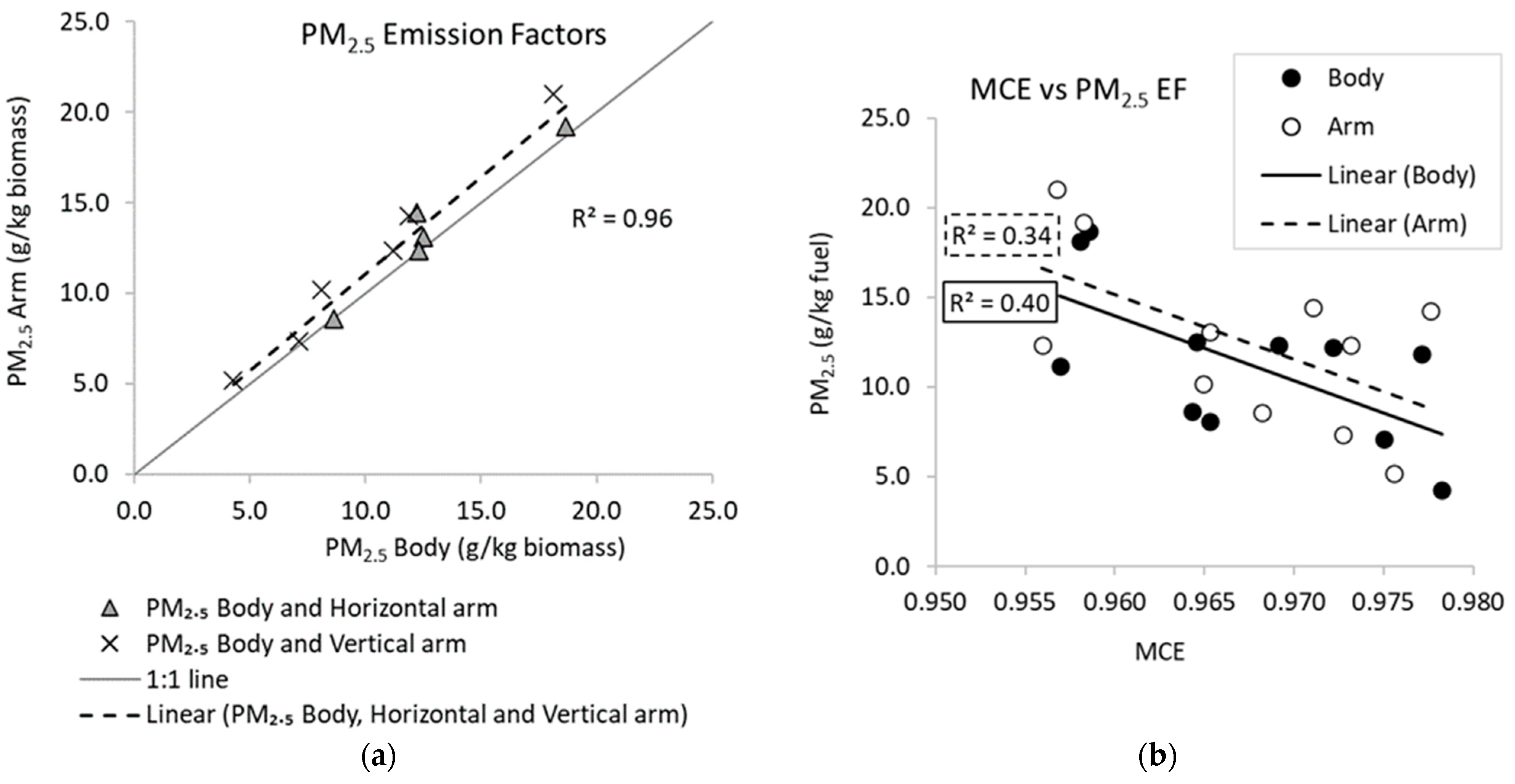
Single-factor ANOVA analyses showed no significant differences between the PM2.5 emission factors (1 Hz) derived from the arm, either vertical or horizontal, and those emission factors derived from the body (PM2.5 body 11.4 ± 4.4 g/kg fuel, PM2.5 arm 12.5 ± 4.7 g/kg fuel: p = 0.6, F/Fcrit = 0.09; body vs. horizontal arm PM2.5 p = 0.79, F/Fcrit = 0.02, body vs. vertical arm PM2.5 p = 0.6, F/Fcrit = 0.06). The related correlation plot showed an R2 of 0.96 (p < 0.001, RMSE = 1.5 g/kg fuel), as shown in Figure 11a. The PM2.5 emission factor ranging from 4.3 to 18.7 g/kg fuel is due to the typical inverse relationship between the combustion quality, measured as MCE, and the pollutants, as shown in Figure 11b. The ranges in the emission factors are due to changes in the combustion conditions affecting the burn quality. PM2.5 emission factors from prescribed biomass burns decrease with increased MCE [29,30].
4. Discussion
The potential effects of rotor wash on air concentration measurements must consider the source characteristics, the performance characteristics of the sensor/sampler, the site meteorological characteristics, and the objective of the sampling. Discrete sources, such as from tracer releases or stacks, may have extreme concentration gradients between ambient air and the plume, leading to large changes in concentrations when the UAS position allows rotor entrainment of ambient air into the plume. The response time of the sensors to these rapidly changing concentrations must be considered, as was examined by the laboratory simulation, where the supply test gas source was moved back and forth across the two sensors’ inlets. Larger area sources, such as landfill emissions or forest fires, are likely to have less discrete concentration gradients with ambient air due to more complete mixing, especially when sampled further downwind or further aloft. This scenario was simulated in the OBTF testing, in contrast to the bench-top laboratory testing, where substantial mixing occurred prior to the gases and particles reaching the sensors. Sampling close to surfaces, such as agricultural lands or fires, can affect measurements as rotor wash impinges on the source surface. This is particularly true for combustion sources, where the downdraft from the rotor wash is likely to affect the combustion efficiency of the fire, or from hard surfaces, where particles are likely to be stirred up by the air movements.
The effect of concentration gradients can only be assessed if the sampling rate of the sensor/sampler is less than the temporal change. Sensors, such as electrochemical sensors, often have induction and recovery periods on the order of seconds. Use of extension arms with sampling tubes also introduces tube transport residence times that slow the responses, although testing here with a 1.37 m tube had no statistically significant effect on the results. Meteorological effects of wind turbulence can alter the degree of mixing, affecting the magnitude of any concentration gradients that can be influenced by rotor wash-induced entrainment.
Finally, the effects of rotor wash need to be considered in view of the objectives of the sampling. Time-averaged concentrations are less likely to be affected than those of instantaneous and spatially resolved concentrations, particularly as the time period of sampling increases. An increased concentration averaging duration from 1 to 10 s was shown to improve the correlation between the body- and arm-mounted sensors. Measurements of concentration ratios, where one concentration is compared to another, are also less likely to be affected when mixing does not result in preferential displacement of one species from the other. This is particularly important when emission ratios are used to determine emission factors, such as in Gullett et al. [16].
5. Conclusions
Tests using two sets of sensors (CO, CO2, and PM2.5) were tested in a laboratory, combustion chamber, and field setting to determine the potential effects of UAS rotor wash on both gas and particle concentration results. The sensors were tested for comparability in the laboratory before being subjected to more rigorous field analyses. The body-mounted sensors on the undercarriage of the UAS compared well with either vertical or horizontal arm-mounted sensors conducting simultaneous measurements during relatively stationary UAS flights in field combustion plume testing. R2 values of 0.90, 0.91, and 0.85 were obtained for the arm-mounted and body-mounted sensors with 1 Hz ∆CO2, ∆CO, and PM2.5 concentration values, respectively. These correlations from the turbulent combustion plume decreased from the R2 values obtained in a well-mixed combustion chamber of 0.97, 0.98, and 0.98, respectively. Increasing the averaging time of the field-derived UAS PM2.5 concentrations from 1 s to 10 s improved the body and arm R2 value to 0.95. The comparability between the body- and arm-mounted concentrations suggests that, for scenarios where short averaging time concentrations are not required, such as the determination of emission factors or whole-area flux calculations, arm-mounted sensors to avoid rotor wash are likely unnecessary for both gas and particle measurements.
Author Contributions
Conceptualization, J.A. and B.K.G.; Methodology, J.A. and B.K.G.; Software, J.A.; Validation, J.A.; Formal Analysis, J.A.; Investigation, J.A. and B.K.G.; Resources, J.A. and B.K.G.; Data Curation, J.A. and B.K.G.; Writing—Original Draft Preparation, J.A. and B.K.G.; Writing—Review & Editing, J.A. and B.K.G.; Visualization, J.A.; Supervision, B.K.G.; Project Administration, B.K.G.; Funding Acquisition, B.K.G. All authors have read and agreed to the published version of the manuscript.
Funding
This work has been supported by the US Department of Defense Strategic Environmental Research and Development Program: RC20-1304, by the US Environmental Protection Agency: Regional and Applied Research Effort: 1763 and 2142, and by the US Environmental Protection Agency Office of Research and Development.
Data Availability Statement
Data used in the writing of this article are available at the US Environmental Protection Agency’s Environmental Dataset Gateway (https://edg.epa.gov).
Acknowledgments
We are grateful for site support from personnel at Tall Timbers Research Station and UAS pilot support from personnel at the University of North Carolina Institute of Environment.
Conflicts of Interest
The authors declare no conflicts of interest.
References
- Chang, C.-C.; Wang, J.-L.; Chang, C.-Y.; Liang, M.-C.; Lin, M.-R. Development of a multicopter-carried whole air sampling apparatus and its applications in environmental studies. Chemosphere 2016, 144, 484–492. [Google Scholar] [CrossRef]
- Schuyler, T.J.; Guzman, M.I. Unmanned Aerial Systems for Monitoring Trace Tropospheric Gases. Atmosphere 2017, 8, 206. [Google Scholar] [CrossRef]
- Villa, T.F.; Salimi, F.; Morton, K.; Morawska, L.; Gonzalez, F. Development and Validation of a UAV Based System for Air Pollution Measurements. Sensors 2016, 16, 2202. [Google Scholar] [CrossRef]
- Burgues, J.; Marco, S. Environmental chemical sensing using small drones: A review. Sci. Total Environ. 2020, 748, 141172. [Google Scholar] [CrossRef] [PubMed]
- Lambey, V.; Prasad, A.D. A Review on Air Quality Measurement Using an Unmanned Aerial Vehicle. Water Air Soil Pollut. 2021, 232, 109. [Google Scholar] [CrossRef]
- Crazzolara, C.; Ebner, M.; Platis, A.; Miranda, T.; Bange, J.; Junginger, A. A new multicopter-based unmanned aerial system for pollen and spores collection in the atmospheric boundary layer. Atmos. Meas. Tech. 2019, 12, 1581–1598. [Google Scholar] [CrossRef]
- Eu, K.S.; Yap, K.M. Chemical plume tracing: A three-dimensional technique for quadrotors by considering the altitude control of the robot in the casting stage. Int. J. Adv. Robot. Syst. 2018, 15. [Google Scholar] [CrossRef]
- Eu, K.S.; Yap, K.M.; Tee, T.H. An Airflow Analysis Study of Quadrotor Based Flying Sniffer Robot. In Proceedings of the 3rd International Conference on Advances in Mechanics Engineering (ICAME), Hong Kong, China, 28–29 July 2014; pp. 246–250. [Google Scholar]
- Koziar, Y.; Levchuk, V.; Koval, A. Quadrotor Design for Outdoor Air Quality Monitoring. In Proceedings of the 39th IEEE International Conference on Electronics and Nanotechnology (ELNANO), Kyiv, Ukraine, 16–18 April 2019; pp. 736–739. [Google Scholar]
- Kuantama, E.; Tarca, R.; Dzitac, S.; Dzitac, I.; Vesselenyi, T.; Tarca, I. The Design and Experimental Development of Air Scanning Using a Sniffer Quadcopter. Sensors 2019, 19, 3849. [Google Scholar] [CrossRef] [PubMed]
- Luo, B.; Meng, Q.H.; Wang, J.Y.; Ma, S.G. Simulate the aerodynamic olfactory effects of gas-sensitive UAVs: A numerical model and its parallel implementation. Adv. Eng. Softw. 2016, 102, 123–133. [Google Scholar] [CrossRef]
- Alvarado, M.; Gonzalez, F.; Erskine, P.; Cliff, D.; Heuff, D. A Methodology to Monitor Airborne PM<sub>10</sub> Dust Particles Using a Small Unmanned Aerial Vehicle. Sensors 2017, 17, 343. [Google Scholar] [CrossRef] [PubMed]
- Burgués, J.; Esclapez, M.D.; Doñate, S.; Pastor, L.; Marco, S. Aerial Mapping of Odorous Gases in a Wastewater Treatment Plant Using a Small Drone. Remote Sens. 2021, 13, 1757. [Google Scholar] [CrossRef]
- Neumann, P.P.; Asadi, S.; Lilienthal, A.J.; Barholmai, M.; Schiller, J.H. Micro-Drone for Wind Vector Estimation and Gas Distribution Mapping. J. IEEE Robot. Autom. Mag. 2011, 6, 1–11. [Google Scholar]
- Li, C.Q.; Han, W.T.; Peng, M.M.; Zhang, M.F.; Yao, X.M.; Liu, W.S.; Wang, T.H. An Unmanned Aerial Vehicle-Based Gas Sampling System for Analyzing CO2 and Atmospheric Particulate Matter in Laboratory. Sensors 2020, 20, 1051. [Google Scholar] [CrossRef]
- Gullett, B.; Aurell, J.; Mitchell, W.; Richardson, J. Use of an unmanned aircraft system to quantify NOx emissions from a natural gas boiler. Atmos. Meas. Tech. 2021, 14, 975–981. [Google Scholar] [CrossRef] [PubMed]
- Arroyo, P.; Gómez-Suárez, J.; Herrero, J.L.; Lozano, J. Electrochemical gas sensing module combined with Unmanned Aerial Vehicles for air quality monitoring. Sens. Actuators B Chem. 2022, 364, 131815. [Google Scholar] [CrossRef]
- Haas, P.; Balistreri, C.; Pontelandolfo, P.; Triscone, G.; Pekoz, H.; Pignatiello, A. Development of an unmanned aerial vehicle UAV for air quality measurements in urban areas. In Proceedings of the 32nd AIAA Applied Aerodynamics Conference, Atlanta, GA, USA, 16–20 June 2014. [Google Scholar]
- Samad, A.; Florez, D.A.; Chourdakis, I.; Vogt, U. Concept of Using an Unmanned Aerial Vehicle (UAV) for 3D Investigation of Air Quality in the Atmosphere-Example of Measurements Near a Roadside. Atmosphere 2022, 13, 663. [Google Scholar] [CrossRef]
- Wang, T.H.; Han, W.T.; Zhang, M.F.; Yao, X.M.; Zhang, L.Y.; Peng, X.S.; Li, C.Q.; Dan, X.J. Unmanned Aerial Vehicle-Borne Sensor System for Atmosphere-Particulate-Matter Measurements: Design and Experiments. Sensors 2020, 20, 57. [Google Scholar] [CrossRef] [PubMed]
- Roldán, J.J.; Joossen, G.; Sanz, D.; del Cerro, J.; Barrientos, A. Mini-UAV Based Sensory System for Measuring Environmental Variables in Greenhouses. Sensors 2015, 15, 3334–3350. [Google Scholar] [CrossRef] [PubMed]
- Greene, B.R.; Segales, A.R.; Waugh, S.; Duthoit, S.; Chilson, P.B. Considerations for temperature sensor placement on rotary-wing unmanned aircraft systems. Atmos. Meas. Tech. 2018, 11, 5519–5530. [Google Scholar] [CrossRef]
- Aurell, J.; Gullett, B.K.; Tabor, D. Emissions from southeastern U.S. Grasslands and pine savannas: Comparison of aerial and ground field measurements with laboratory burns. Atmos. Environ. 2015, 111, 170–178. [Google Scholar] [CrossRef]
- Grandesso, E.; Gullett, B.; Touati, A.; Tabor, D. Effect of Moisture, Charge Size, and Chlorine Concentration on PCDD/F Emissions from Simulated Open Burning of Forest Biomass. Environ. Sci. Technol. 2011, 45, 3887–3894. [Google Scholar] [CrossRef] [PubMed]
- Aurell, J.; Gullett, B.; Holder, A.; Kiros, F.; Mitchell, W.; Watts, A.; Ottmar, R. Wildland fire emission sampling at Fishlake National Forest, Utah using an unmanned aircraft system. Atmos. Environ. 2021, 247. [Google Scholar] [CrossRef] [PubMed]
- Zhou, X.; Aurell, J.; Mitchell, W.; Tabor, D.; Gullett, B. A small, lightweight multipollutant sensor system for ground-mobile and aerial emission sampling from open area sources. Atoms. Environ. 2017, 154, 31–41. [Google Scholar] [CrossRef] [PubMed]
- U.S. EPA OTM-48. Emission Factor Determination by the Carbon Balance Method. 2022. Available online: https://www.epa.gov/emc/emc-other-test-methods (accessed on 10 January 2024).
- Seltman, H.J. Experimental Design and Analysis. Carnegie Mellon University. 2015. Available online: http://www.stat.cmu.edu/~hseltman/309/Book/Book.pdf (accessed on 10 January 2024).
- Aurell, J.; Gullett, B.; Grier, G.; Holder, A.; George, I. Seasonal emission factors from rangeland prescribed burns in the Kansas Flint Hills grasslands. Atmos. Environ. 2023, 304, 119769. [Google Scholar] [CrossRef] [PubMed]
- Hosseini, S.; Urbanski, S.P.; Dixit, P.; Qi, L.; Burling, I.; Yokelson, R.; Shrivastava, M.; Jung, H.; Weise, D.R.; Miller, W.; et al. Laboratory characterization of PM emissions from combustion of wildland biomass fuels. J. Geophys. Res. Atmos. 2013, 118, 9914–9929. [Google Scholar] [CrossRef]
Figure 1.
UAS and Kolibri sampling package with the (a) vertical arm and (b) horizontal arm. (c) Kolibri (black box) with side-by-side SidePaks for sensor comparison inside the OBTF.
Figure 1.
UAS and Kolibri sampling package with the (a) vertical arm and (b) horizontal arm. (c) Kolibri (black box) with side-by-side SidePaks for sensor comparison inside the OBTF.

Figure 2.
Schematic of the two sensor sets’ location and inlets. Not to scale.

Figure 3.
Sensor correlation plots: (a) CO2 and (b) CO sensor measurements at three different concentrations (500, 1000, and 2000 ppm CO2, and 10, 40, and 70 ppm CO).
Figure 3.
Sensor correlation plots: (a) CO2 and (b) CO sensor measurements at three different concentrations (500, 1000, and 2000 ppm CO2, and 10, 40, and 70 ppm CO).

Figure 4.
Line plot and scatter plot of traces of CO2 (a,c) and CO (b,d) using calibration gases.

Figure 5.
Response time curve for the two CO2 sensors, one with an analog signal channel and one with a digital signal channel.
Figure 5.
Response time curve for the two CO2 sensors, one with an analog signal channel and one with a digital signal channel.

Figure 6.
Correlation plots of CO2 and CO sensors from laboratory biomass burns (a,c) without arm tubing and (b,d) with arm tubing on one of the two sensors.
Figure 6.
Correlation plots of CO2 and CO sensors from laboratory biomass burns (a,c) without arm tubing and (b,d) with arm tubing on one of the two sensors.


Figure 7.
Correlation plots of side-by-side SidePak PM2.5 measurements: (a) three burns, both SidePaks without arm tubing; (b) three burns, one SidePak with sampling tubing (arm simulation) compared to one SidePak without sampling tubing (body-mounted simulation); (c) all tests; (d) PM2.5 emission factors from all six laboratory biomass burns.


Figure 8.
Example of (a) CO2 and (b) CO concentration traces of the two pairs of sensors, one mounted on the sampling arm and one mounted on the UAS body, from a single field burn with their respective correlation plots, (c) CO2 and (d) CO.
Figure 8.
Example of (a) CO2 and (b) CO concentration traces of the two pairs of sensors, one mounted on the sampling arm and one mounted on the UAS body, from a single field burn with their respective correlation plots, (c) CO2 and (d) CO.

Figure 9.
Average (a) ∆CO2 and (b) ∆CO values from each field burn.

Figure 10.
Typical field results with the UAS. (a) PM2.5 concentration traces from the two pairs of PM2.5 instruments, one sampling tube inlet mounted on a vertical arm, one body mounted, from a typical field burn, and its respective correlation plot; (b) every second data and (c) 10 s average; (d) average PM2.5(t) values from each field burn.

Figure 11.
(a) PM2.5 emission factor derived from horizontal and vertical arm position versus body, and (b) PM2.5 emission factor versus MCE.
Figure 11.
(a) PM2.5 emission factor derived from horizontal and vertical arm position versus body, and (b) PM2.5 emission factor versus MCE.


Table 1.
Measured parameters and instrument.
| Measured Parameter | Instrument/ Equipment | Method | Flow Rate/ Sampling Rate |
|---|---|---|---|
| CO2 | CO2 Engine® K30 FR | NDIR | 1 L/min, 1 Hz |
| CO | EC4-500-CO | Electrochemical cell | 1 L/min, 1 Hz |
| PM2.5 Batch | SKC Personal Modular Impactor (PMI) | 37 mm Teflon filter/ gravimetric | 3 L/min |
| PM2.5 Time-Resolved | SidePak™ AM520 | 90° light-scattering | 1.7 L/min, 1 Hz |
Disclaimer/Publisher’s Note: The statements, opinions and data contained in all publications are solely those of the individual author(s) and contributor(s) and not of MDPI and/or the editor(s). MDPI and/or the editor(s) disclaim responsibility for any injury to people or property resulting from any ideas, methods, instructions or products referred to in the content. |
© 2024 by the authors. Licensee MDPI, Basel, Switzerland. This article is an open access article distributed under the terms and conditions of the Creative Commons Attribution (CC BY) license (https://creativecommons.org/licenses/by/4.0/).
Share and Cite
MDPI and ACS Style
Aurell, J.; Gullett, B.K. Effects of UAS Rotor Wash on Air Quality Measurements. Drones 2024, 8, 73. https://doi.org/10.3390/drones8030073
AMA Style
Aurell J, Gullett BK. Effects of UAS Rotor Wash on Air Quality Measurements. Drones. 2024; 8(3):73. https://doi.org/10.3390/drones8030073
Chicago/Turabian StyleAurell, Johanna, and Brian K. Gullett. 2024. "Effects of UAS Rotor Wash on Air Quality Measurements" Drones 8, no. 3: 73. https://doi.org/10.3390/drones8030073