
UDE-Based Dynamic Surface Control for Quadrotor Drone Attitude Tracking under Non-Ideal Actuators

1
School of Aeronautics and Astronautics, University of Electronic Science and Technology of China, Chengdu 611731, China
2
Aircraft Swarm Intelligent Sensing and Cooperative Control Key Laboratory of Sichuan Province, Chengdu 611731, China
*
Author to whom correspondence should be addressed.
Drones 2023, 7(5), 305; https://doi.org/10.3390/drones7050305
Submission received: 31 March 2023
/
Revised: 22 April 2023
/
Accepted: 2 May 2023
/
Published: 5 May 2023
Abstract
:Quadrotor drone attitude tracking is inevitably affected by the combination of model uncertainties, external disturbances, and non-ideal actuator dynamics during stable flight and complex maneuvers. In order to achieve precise attitude control in these situations, a cascade-structured dynamic surface control (DSC) strategy is proposed based on an uncertainty and disturbance estimator (UDE), considering the actuator dynamics as represented by a first-order plus time-delay model. The DSC scheme is used to transform the original attitude dynamics system into a set of interconnected subsystems. On the one hand, the mismatched disturbances in the attitude kinematics and dynamics loops are converted into matched disturbances to accommodate the structural constraints of the UDE so that these disturbances, as well as the non-ideality caused by the actuator time delay, are estimated and compensated for by the approach. On the other hand, the “complexity explosion” problem is addressed by the first-order filter employed by DSC. The ultimate boundedness of the closed-loop system is proven while the parameter design constraints are provided. MATLAB Simulink simulations are conducted to demonstrate the desirability of considering actuator dynamics and to verify that the proposed control strategy can relax the constraints of the control parameters and enable a higher accuracy.
1. Introduction
In recent years, quadrotor drones have gained increasing popularity due to their versatility, agility, low cost, and flexible deployment [1]. They have been widely used in various applications such as aerial photography, delivery, search and rescue, and surveillance [2,3,4,5]. To complete these missions, precise attitude control is critical for quadrotor drones to achieve stable flight and perform complicated maneuvers. Many researchers have conducted extensive and in-depth research on the attitude control of quadrotor drones and have proposed various control schemes based on different control methods [6,7,8,9,10].
However, there are inherent model uncertainties in practice, including coupling and nonlinearity in the quadrotor drone attitude dynamics model, as well as immeasurable external disturbances in complex operating environments. The rejection of these unfavorable uncertainties and disturbances has become a primary goal in the design process of attitude tracking controllers to ensure that the system is stable and attains a high level of accuracy. Various methods have been suggested to address this issue. To improve the transient performance and rapidly converge to stability when faced with perturbations, Noordin et al. [11] proposed an adaptive proportional integral derivative (PID) control scheme based on second-order sliding mode control (SMC) for tuning parameter gains. Additionally, a fuzzy compensator was employed to mitigate chattering phenomena. In [12], a model-based control method combining Active Disturbance Rejection Control (ADRC) and Embedded Model Control (EMC) was developed for the complete digital attitude control unit for a quadrotor drone. The model uncertainties could be accurately estimated or dismissed by this algorithm, and a simplified controllable model was thus obtained. Castillo et al. [13] presented a quaternion-based Disturbance Observer-Based (DOB) controller for quadrotor drones to estimate and compensate for the external disturbances and the Coriolis term, allowing precise and aggressive attitude maneuvers in highly disturbed environments. In [14], a global non-singular attitude tracking controller was proposed, which utilizes the uncertainty and disturbance estimator (UDE) and introduces unit quaternion to effectively overcome the effects of system coupling, model uncertainties, and external disturbances.
Among the aforementioned disturbance rejection methods, UDE-based control enables rapid estimation of uncertainties and disturbances by designing appropriate filters for a wider class of systems [15] and has the advantages of structural simplicity and ease of implementation [16]. UDE-based control was originally proposed in [16] to conquer the intrinsic weaknesses of time delay control (TDC). In recent years, this approach has been used successfully in many applications in various fields, such as time-delayed processes [17], vehicle systems without velocity measurements [18,19,20], and multi-vehicle systems [19,21]. In addition, with the aim of simultaneously rejecting system disturbances and velocity measurement noise, a robust control scheme combining a noise estimator (NE) with a UDE was developed in [22] and was shown to provide excellent trajectory tracking performance. However, due to the structural constraints, the mismatched uncertainties and disturbances, e.g., the kinematic couplings and the external disturbance torque in the model of quatortor drone attitude dynamics, cannot be handled by traditional UDE [23]. In order to compensate for the shortcomings and expand the application scenarios of UDE, the back-stepping method was introduced into the UDE-based control scheme [14,23,24]. Specifically, in [14,23,24], a high-order nonlinear system with mismatched disturbances was decomposed into multiple subsystems with lower order and matched disturbances by the back-stepping method. Thus, the structural constraints of UDE are removed during the design of each subsystem controller. However, in the back-stepping method, the controller of each subsystem requires the derivative of the virtual control signal of the upper-level subsystem as a feed-forward signal. The differentiation process makes the calculation complex and arduous, leading to the “complexity explosion” disadvantage [24]. In [23], a reference model was utilized to relax the derivative calculation of the virtual controls, avoiding the “complexity explosion” problem, but in the ultimate boundedness analysis, the boundedness of the UDE estimation error for each subsystem was not rigorously demonstrated. In addition, methods such as command filtering back-stepping control [25] and dynamic surface control [26] have also been used to address such issues. However, it is still challenging yet important for quadrotor drone systems to deal with the complexity explosion problem during the design of UDE-based high-precision attitude controllers.
Meanwhile, the actuator is a critical component of quadrotor drones, responsible for translating the control input of the flight controller into the forces and torques that drive the motion. The actuator dynamics contain a non-negligible transient response, which can significantly affect the stability, controllability, and agility of the control system. Therefore, it should be taken into account when designing the attitude controller of the quadrotor drone, especially for fast maneuvers [13]. However, few of the above studies, as well as other relevant applications, have considered attitude control strategies that take into account the actuator performance, but rather assume that the actuator dynamics are ideal, i.e., fast enough to be negligible compared to the dynamics of the outer-loop system [27,28,29]. Ignoring the actuator dynamics during control design can result in a significant deterioration in performance or even a loss of stability. This is because the relationship between the controller parameters and the system bandwidth needs to adhere to the limitations imposed by the dynamics of the actuator to guarantee system stability, as demonstrated in the author’s previous work [30]. In most cases, actuator dynamics are approximated by a first-order model [31,32,33,34]. Nevertheless, in the studies conducted by Qi et al. [35] and Qin et al. [24], the actuators are described as first-order plus time-delay (FOPTD) models by using thrust test platforms to precisely identify the model parameters, which are more consistent with the actual quadrotor drone actuator characteristics. With a high-accuracy actuator dynamic model, a modified uncertainty and disturbance estimator (MUDE) has been developed to estimate and compensate for not only the lumped disturbances in the attitude and actuator dynamics but also the actuator time delay [35]. However, in this work, the attitude kinematic couplings were ignored by applying a small angle approximation, and the second-order filter adopted in this paper increases the complexity of the system. Qin et al. [24] presented a controller based on a cascade-modified uncertainty and disturbance estimator (CMUDE), leveraging the back-stepping methods for quadrotor drone attitude tracking under exogenous disturbance and non-ideal actuators. However, in this method, the derivatives of the mismatched disturbances need to be estimated and reconstructed, which also complicates the structure of the controller.
To the best of our knowledge, there is a lack of research on UDE-based attitude control strategies for quadrotor drones that not only utilize actuator dynamic models in the controller design to improve control accuracy but also deal with the mismatched disturbances as well as the complexity explosion issue. This study attempts to fill this gap. The main purpose of this work is to develop a UDE-based dynamic surface control strategy with a simple and intuitive cascade structure for quadrotor drone attitude control under non-ideal actuators of the FOPTD model. The introduction of a dynamic surface transforms the original attitude dynamics system into a set of interconnected subsystems, turning the mismatched disturbances in the attitude kinematics and dynamics loops into matched disturbances. As a result, UDE can be implemented in each subsystem to estimate the lumped disturbances that are used for disturbance compensation in feedback control, leading to an improved control accuracy and robustness. Meanwhile, the non-ideality induced by the time delay of the actuator, which is confirmed to be unignorable by experimental evidence [35], is also estimated and compensated for by the approach. Unlike back-stepping control, the dynamic surface control method employs a first-order filter to construct the derivative of the virtual control, thereby avoiding the problem of a “complexity explosion”. Specifically, compared with MUDE [35] and CMUDE [24], the incorporation of dynamic surfaces avoids the complex estimation or reconstruction of derivatives of the disturbances in the subsystems, and consequently provides a simple and intuitive structure that is easier to implement. A comparison with three-channel attitude tracking numerical simulations verifies the necessity of considering the actuator dynamics in the controller design process, as well as the fact that the proposed control strategy relaxes the value range of the control parameters and enables a higher control accuracy. The main contributions of this paper are summarized as follows:
- (1)
- A cascade-structured, UDE-based dynamic surface controller is proposed to address the issues of mismatched disturbance and complexity explosion, which is characterized by its simple structure and easy implementation in a quadrotor drone system, thus increasing the robustness and accuracy of the attitude control system.
- (2)
- A rigorous proof of the ultimate boundedness of the closed-loop system is given by a mathematical analysis, especially based on the small gain theorem, while the stability conditions and constraints of the controller parameters are provided, indicating that the parameters of the different loops can be designed independently.
- (3)
- In the design process of the controller, the non-ideal actuator with the FOPTD dynamic model is fully considered to eliminate the parameter constraints of the outer-loop controller brought by the actuator dynamics and improve the attitude control accuracy.
In the following sections, the paper is structured as follows: Section 2 formulates a quadrotor drone attitude dynamics model with actuator dynamics. The proposed controller design and stability analysis are presented in Section 3. Section 4 presents the numerical simulation results. Finally, Section 5 summarizes the conclusions.
2. Modeling
The modeling of quadrotor drones has been elaborated in [36,37,38,39,40,41]. In this section, referring to the models in the above literature, the attitude dynamics model of the quadrotor drone will be established in the presence of model uncertainties, input disturbances, and actuator dynamics.
2.1. Quadrotor Drone Kinematics and Dynamics Model
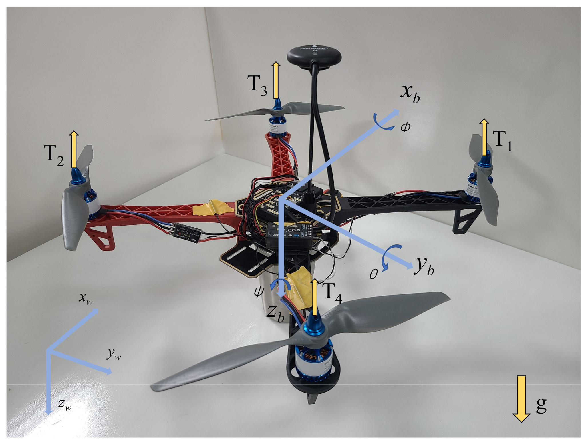
Quadrotor systems are often represented by an inertial coordinate system and a body-fixed coordinate system [37]. The quadrotor drone with an X-configuration considered in this paper is illustrated with the body-fixed coordinate system in Figure 1. Assuming that the quadrotor drone is a rigid body, the attitude of the quadrotor drone is represented by Euler angles , with the three components denoting the roll angle, pitch angle, and yaw angle, respectively. Considering the rotation from the inertial frame to the body frame in the order of Z–Y–X, the attitude kinematics of the quadrotor drone can be expressed as:
where represents the angular rate of the quadrotor drone in the fixed-body frame. It can be seen that the kinematics Equation (1) reflects the nonlinear relation between the Euler angle rates and the body angular rates .
Normally, the attitude dynamics of the quadrotor drone decomposed in the body frame is given by the following equation:
where is the quadrotor drone moment of inertia about its center of mass located in the origin of the body coordinate system; is the external disturbance torque, such as the asymmetric torque, the rotational inertia torque, and the air-drag torque; and is the control torque produced by the quadrotor drone motors.
To facilitate the controller design, we rewrite the kinematics Equation (1) and dynamics Equation (2) with a strict feedback form in the state space:
where
Normally, and are reffered to as the lumped disturbance of the corresponding subsystem.
Note that in Equation (3), all three attitude channels, i.e., the rows of the state equation, have the same dynamics form. For simplicity, each channel can be expressed in the following second-order form without any loss of generality.
where denotes the Euler angle of a certain channel, is the corresponding angular velocity, and are the lumped disturbances in the angular motion, and is the virtual input of the same channel, which is proportional to the real torque with a proportionality coefficient equal to the reciprocal of the moment of inertia.
Remark 1.
In studies that ignore actuators, is considered equal to the control input generated by the controller, whereas in reality, there is a difference between and the system input due to the presence of actuator dynamics. It can be understood as follows: the system input generated by the controller is the input of the actuator, while is the output of the actuator and also the real torque that drives the quadrotor attitude change. Therefore, the actuator needs to be modeled next. Furthermore, the input of the actuator is the real input of the whole system.
2.2. Actuator Model
In our work, the actuator dynamics of each attitude channel are considered as a first-order plus time-delay model, as follows:
where denotes the actuator output, i.e., the actual torque applied to each channel to generate attitude motions; is the actuator input, i.e., the torque command generated by the controller; and are the parameters of the actuator model, which represent the time constant and the time delay, respectively; and stands for the lumped disturbance that encompasses the immeasurable external disturbance and the uncertainty in the model.
Remark 2.
In practice, the parameters and can be identified precisely, and thus the nominal actuator model, as is shown in Equation (6), with in (5), can be fully utilized in the controller design process to improve the control accuracy. Furthermore, this nominal model can be used as an estimator to obtain the torque produced by the actuator [35].
By combining (4) and (5), a third-order attitude dynamic model with actuator dynamics can be obtained, as expressed in the following equation.
where is the virtual input of the third-order system and is the lumped disturbance in the equivalent actuator equation.
A standard assumption on the system (7) is listed as follows.
Assumption 1.
, , and are bounded.
3. UDE-Based Dynamic Surface Controller Design
The dynamics of each attitude channel take the form of (7). Without loss of generality, we design a control law for (7) such that the attitude state can track a desired attitude signal . Then, the identical controller architecture can be employed for each attitude channel, albeit with distinct control gains.
Thus, the control objective can be described as ensuring the tracking errors of the closed-loop system satisfy
where denotes the specified ultimate bound of the tracking errors and is the corresponding settling time.
3.1. Step 1
Define the first dynamic surface, which is the tracking error of for its desired trajectory , as
Then, the first equation in (7) can be rewritten as
In (10), is considered as a virtual control input.
Firstly, we find a stabilizing control law for the subsystem (10):
where denotes the estimation of estimated by UDE. The control law given by Equation (11) consists of two components: a nominal proportional controller augmented with a feedforward term and a compensation term produced by UDE. The latter is designed to counteract the influence of the lumped disturbance .
The conventional UDE method is employed to calculate . Throughout the remainder of this paper, corresponding uppercase letters will be used to represent the Laplace transform of the signals. In the frequency domain, the estimate for can be formulated as follows:
From (14), we derive that
Define in such a way that
where is a positive parameter to be designed.
Remark 3.
It can be seen that is obtained by passing through a first-order filter and is the filter time constant. From (16), the feedforward term subsequently used in the next step can be derived as
The introduction of this filter, which is the essence of dynamic surface control, overcomes the “complexity explosion” problem that arises from taking the derivative of the virtual control.
Define the second surface error to be
and the error between and to be
Introducing the changes in variables (18) and (19) into (10) and combining with (15) and (16), the error dynamics satisfy
where
, , , , and denotes the estimation error of UDE.
The characteristic polynomial of is
The Routh criterion dictates that is Hurwitz if and only if the subsequent stability conditions are met:
Lemma 1.
Proof of Lemma 1.
It is known that is Hurwitz under the conditions in (22). As is stated in Theorem 4.5 of [42], the unforced system
is globally asymptotically stable at the origin equilibrium point. Based on Lemma 4.6 in the same reference [42], the global ISS of system (20) is guaranteed. Subsequently, the stability of (20) in a BIBS sense can be established by referring to the analysis on page 174 in [42]. □
3.2. Step 2
In the second step, a control law is designed as the virtual input of the second equation of (7) to guarantee the boundedness of as well as .
takes the same structure as to stabilize the subsystem (24):
where denotes the estimation of generated by UDE.
Another first-order filter is considered to estimate , satisfying the following equation:
The filter is designed as the following first-order form:
Then,
which can be transformed to the time domain as
Define in such a way that
where is a positive parameter to be designed as the time constant of the first-order filter.
Let the third surface error be
and the error between and be
Considering the changes in variables (31) and (32) in (24) and combining with (29), (30), and (20), yields
where , , , ,
, and denotes the estimation error of UDE.
Since has the same structure as , it can be easily derived that is Hurwitz if and only if the following stability conditions are satisfied:
Combining (20) with (33), the error dynamics of the entire closed-loop system can be described as
where .
Lemma 2.
Proof of Lemma 2.
With , , , and as inputs, the unforced system of (35) is
and are the transfer matrices of the two subsystems in (36), respectively. Under the stability conditions (22) and (34), and are Hurwitz. It is clear that the corresponding transfer matrices are proper and real rational stable, i.e., . Then, according to Theorem 9.1 (Small Gain Theorem) in [43], the interconnected system (36) is internally stable if and only if
Therefore, we shall prove that (37) can be satisfied.
The Hamiltonian matrices of and are denoted by and :
By Lemma 4.7 in [43], it can be derived that and are satisfied if and only if and have no eigenvalues on the imaginary axis, respectively. The characteristic polynomials of and , respectively, are
and
where
It can be seen from Equations (39) and (40) that if , then it is impossible for there to be any eigenvalues on the imaginary axis that satisfy and . Therefore, under the following condition
(37) is satisfied and thus the system (35) is internally stable. Furthermore, the state matrix is a Hurwitz matrix according to Lemma 5.2 in [43].
Combining (22), (34), and (42) yields the following comprehensive conditions to guarantee that is Hurwitz:
Then, the remaining proof for the ISS and BIBS stability of (35) is the same as the proof process presented in Lemma 1. □
Up to this point, the controller for the second loop of system (7) has been obtained, which consists of (25), (29), and (30) with parameters constrained by (44). The controller is cascaded with the controller designed in the previous step, ensuring the boundedness of the tracking error when , , , and are bounded.
3.3. Step 3
Finally, the input u in the last equation of (7) should be designed to guarantee the boundedness of .
The structure of u is analogous to the previous steps in order to stabilize the subsystem (45):
where is the estimation of estimated by UDE.
Similar to the preceding, is estimated by UDE through the following approach
From (49), we derive that
The dynamics of the tracking error and the UDE estimation error satisfy
where , , .
It is clear that and are the two eigenvalues of . According to the Routh criterion, is Hurwitz if and only if
Theorem 1.
Proof of Theorem 1.
Rewrite (53) into the compact form:
where , , , and .
Under conditions (55), it is easy to verify that is Hurwitz by considering the characteristic polynomials of as
Therefore, with the assistance of the results obtained in Lemma 1 and Lemma 2, the proof of the ISS and BIBS stability of (54) can be provided in the same way as in Lemma 1.
Now, we choose a Lyapunov function candidate V as
Then, the derivative of V is given by
where is the maximum eigenvalue of and is an auxiliary parameter. Then,
for all . According to the conditions of Theorem 4.19 in [42], is the bound of the zero-state response of system (54). is Hurwitz under (55); thus, the zero-input response of (54) decays to zero exponentially fast. Hence, for any initial condition and any given positive constant C, there exists a such that
Thus, can be the ultimate bound of the attitude tracking error since .
It can be seen that the bound is proportionate to , with a proportionality coefficient of . As part of the denominator,
where is the trace of matrix .
Equation (61) shows that is an adjustable bound by tuning the filter parameters , , and . The smaller the filter parameters, the smaller the boundary. □
Up to now, the UDE-based dynamic surface control law for the entire attitude tracking system (7) has been obtained, consisting of three fundamental control frameworks ((11), (25), and (46)), three UDEs ((15), (29), and (50)), and two filters ((16) and (30)). The control parameters are constrained by conditions (55) to guarantee the boundedness of the tracking error under Assumption 1. All filters used in the control law are of first-order structure.
Remark 4.
Remark 5.
Five first-order filters are used in the controller of this paper, three of which are introduced by UDEs and two by DSC. Compared with the MUDE in [35], which employs a second-order UDE filter to estimate , and the CMUDE in [24], which uses a complex structure to reconstruct , , and , the structure of the method proposed in this paper has the advantage of being simpler and more intuitive.
4. Simulation Results
In this section, the simulation results of three-channel quadrotor drone attitude tracking are presented to illustrate how the proposed control strategy improves the control performance when subjected to non-ideal actuators and lumped disturbances. In the simulations, the proposed UDE-based dynamic surface control (denoted as DSUDE) strategy is compared with two other control strategies, one of which is the reduced DSUDE (denoted as RDSUDE) strategy with the same structure as DSUDE but ignoring the actuator dynamics, i.e., considering the control input u equal to the actuator output . The other control strategy for comparison is the CMUDE developed in [24].
As shown in Figure 3, the desired trajectories of three control channels in the simulations are , , and , respectively. When the Euler angles vary, cross-coupling occurs and acts as a time-varying disturbance in the corresponding channel. Disturbance torques are added as . The time delay of the actuators is 0.04 s, and the moment of inertia is chosen as . Due to the similar moment of inertia of the three channels, we use the same group of controller feedback gains for all three channels. Taking the pitch channel as an example, the default controller parameters are displayed in Table 1.
Comparative simulation results are shown in Figure 4, Figure 5, Figure 6 and Figure 7. As demonstrated in Figure 4, compared with the RDSUDE method that ignores the actuator dynamics, the DSUDE method that utilizes the actuator dynamic parameters for controller design significantly improves the oscillation characteristics of the attitude tracking, resulting in smoother convergence of the tracking error and improving the robustness of the system. Specifically, when , RDSUDE cannot make the error converge, indicating that the larger the , the more the actuator dynamics cannot be ignored in the controller design process.
Figure 5 shows how different values affect the attitude tracking performance of DSUDE.
It can be seen that, on the one hand, the larger the , the more severe the oscillation of the tracking error and the slower the convergence speed. On the other hand, a smaller leads to a larger overshoot of the tracking error when the desired trajectory varies discontinuously. This is easy to understand because a smaller further amplifies the derivative of the tracking error, resulting in a larger control signal introduced by this derivative term and thus a larger overshoot. In addition, corresponding to Figure 5, Table 2 shows the Root Mean Square (RMS) of the attitude tracking error for the three channels in the 14–16 s interval. In this time period, the attitude tracking process has entered a steady state, indicating that the RMS values characterize the control accuracy of the system. From Table 2, it can be seen that smaller values can obtain a lower RMS of steady-state tracking errors, i.e., a higher tracking accuracy.
Therefore, the trade-off between oscillation, overshoot, and steady-state accuracy should be considered in the parameter design of the DSUDE, and an appropriate value should be chosen to obtain more appropriate control characteristics.
A comparison between DSUDE and CMUDE is shown in Figure 6 and Figure 7. In the comparative simulation, two different groups of control parameters are used. One group of parameters is the default values listed in Table 1, and the other group takes smaller values, as shown in Table 3.
It is evident from Figure 6 that DSUDE and CMUDE exhibit similar attitude tracking errors when they use the default control parameters, but DSUDE produces less transient overshoot when the reference signal encounters a discontinuity. In addition, DSUDE has a larger range of parameter values, and each parameter can take smaller values to obtain smaller tracking errors, which significantly improves the control accuracy. On the contrary, when CMUDE adopts smaller parameters in Table 3, the system appears to be unstable. It is worth noting that, as mentioned in [24], the parameters of CMUDE must satisfy and , while DSUDE does not have similar constraints between the parameters of different loops, e.g., when as shown in Table 3, the control process remains stable. Therefore, compared with CMUDE, DSUDE proposed in this paper has a wider range of parameter values and can obtain a higher attitude tracking accuracy and a stronger robustness.
However, Figure 6 also shows that the oscillation of the transient process can be significant when DSUDE uses smaller parameters. To overcome this drawback, the adaptive parameter method can be considered to increase the control parameters during the oscillation phase.
Figure 7 shows the UDE estimation errors in each loop of DSUDE and CMUDE, taking the pitch channel as an example, which leads to conclusions largely consistent with the above.
5. Conclusions
A UDE-based robust controller combined with a dynamic surface is proposed for the attitude tracking of quadrotor drones, using the actuator dynamic model for controller design and achieving accurate attitude control while rejecting disturbances. The DSC scheme with a cascaded structure addresses both the structural constraints inherent in traditional UDEs and the “complexity explosion” issue. Parameter design constraints are provided while proving the ultimate boundedness of the closed-loop system. Specifically, constraints on the control parameters are relaxed, and the parameters are independent between different loops. Numerical simulations show that by exploiting actuator dynamics and introducing DSC, the proposed controller can significantly improve the control robustness and obtain a greater precision.
Future works include extending this research to the position and attitude control of quadrotor drones, as well as improving the transient performance when discontinuous changes in the reference signal are encountered, and, more specifically, mitigating the apparent oscillations caused by small dynamic surface filter parameters.
Author Contributions
Conceptualization, L.X. and K.Q.; methodology, L.X.; software, L.X. and F.T.; validation, L.X. and F.T.; formal analysis, L.X.; investigation, L.X.; writing—original draft preparation, L.X. and F.T.; writing—review and editing, K.Q., M.S. and B.L.; supervision, K.Q., M.S. and B.L.; funding acquisition, K.Q., M.S. and B.L. All authors have read and agreed to the published version of the manuscript.
Funding
This work was supported in part by the National Natural Science Foundation of Sichuan under Grant No. 2022NSFSC0037, in part by the Science and Technology Department of Sichuan Province under Grant No. 2022JDR0107 and 2021YFG0131, in part by the Fundamental Research Funds for the Central Universities under Grant No. ZYGX2020J020, and in part by the Wuhu Science and Technology Plan Project (2022yf23).
Data Availability Statement
The study did not report any data.
Conflicts of Interest
The authors declare no conflict of interest.
References
- Gupte, S.; Mohandas, P.I.T.; Conrad, J.M. A survey of quadrotor unmanned aerial vehicles. In Proceedings of the 2012 IEEE Southeastcon, Orlando, FL, USA, 15–18 March 2012; pp. 1–6. [Google Scholar]
- Budiharto, W.; Irwansyah, E.; Suroso, J.S.; Chowanda, A.; Ngarianto, H.; Gunawan, A.A.S. Mapping and 3D modelling using quadrotor drone and GIS software. J. Big Data 2021, 8, 48. [Google Scholar] [CrossRef]
- Dalwadi, N.; Deb, D.; Muyeen, S. Adaptive backstepping controller design of quadrotor biplane for payload delivery. IET Intell. Transp. Syst. 2022, 16, 1738–1752. [Google Scholar] [CrossRef]
- Fernández-Guisuraga, J.M.; Sanz-Ablanedo, E.; Suárez-Seoane, S.; Calvo, L. Using unmanned aerial vehicles in postfire vegetation survey campaigns through large and heterogeneous areas: Opportunities and challenges. Sensors 2018, 18, 586. [Google Scholar] [CrossRef] [PubMed]
- Yang, H.C.; AbouSleiman, R.; Sababha, B.; Gjioni, E.; Korff, D.; Rawashdeh, O. Implementation of an autonomous surveillance quadrotor system. In Proceedings of the AIAA Infotech@ Aerospace Conference and AIAA Unmanned… Unlimited Conference, Seattle, WA, USA, 6–9 April 2009; p. 2047. [Google Scholar]
- Zhang, X.; Zhuang, Y.; Zhang, X.; Fang, Y. A novel asymptotic robust tracking control strategy for rotorcraft UAVs. IEEE Trans. Autom. Sci. Eng. 2022, 1–12. [Google Scholar] [CrossRef]
- Duan, X.; Yue, C.; Liu, H.; Guo, H.; Zhang, F. Attitude tracking control of small-scale unmanned helicopters using quaternion-based adaptive dynamic surface control. IEEE Access 2020, 9, 10153–10165. [Google Scholar] [CrossRef]
- Razmi, H.; Afshinfar, S. Neural network-based adaptive sliding mode control design for position and attitude control of a quadrotor UAV. Aerosp. Sci. Technol. 2019, 91, 12–27. [Google Scholar] [CrossRef]
- Chen, Q.; Ye, Y.; Hu, Z.; Na, J.; Wang, S. Finite-time approximation-free attitude control of quadrotors: Theory and experiments. IEEE Trans. Aerosp. Electron. Syst. 2021, 57, 1780–1792. [Google Scholar] [CrossRef]
- Wang, S.; Chen, J.; He, X. An adaptive composite disturbance rejection for attitude control of the agricultural quadrotor UAV. ISA Trans. 2022, 129, 564–579. [Google Scholar] [CrossRef]
- Noordin, A.; Mohd Basri, M.A.; Mohamed, Z. Position and Attitude Tracking of MAV Quadrotor Using SMC-Based Adaptive PID Controller. Drones 2022, 6, 263. [Google Scholar] [CrossRef]
- Lotufo, M.A.; Colangelo, L.; Perez-Montenegro, C.; Canuto, E.; Novara, C. UAV quadrotor attitude control: An ADRC-EMC combined approach. Control Eng. Pract. 2019, 84, 13–22. [Google Scholar] [CrossRef]
- Castillo, A.; Sanz, R.; Garcia, P.; Qiu, W.; Wang, H.; Xu, C. Disturbance observer-based quadrotor attitude tracking control for aggressive maneuvers. Control Eng. Pract. 2019, 82, 14–23. [Google Scholar] [CrossRef]
- Lu, Q.; Ren, B.; Parameswaran, S. Uncertainty and disturbance estimator-based global trajectory tracking control for a quadrotor. IEEE/ASME Trans. Mechatron. 2020, 25, 1519–1530. [Google Scholar] [CrossRef]
- Ren, B.; Zhong, Q.C.; Dai, J. Asymptotic reference tracking and disturbance rejection of UDE-based robust control. IEEE Trans. Ind. Electron. 2016, 64, 3166–3176. [Google Scholar] [CrossRef]
- Zhong, Q.C.; Rees, D. Control of uncertain LTI systems based on an uncertainty and disturbance estimator. J. Dyn. Syst. Meas. Control 2004, 126, 905–910. [Google Scholar] [CrossRef]
- Sun, L.; Li, D.; Zhong, Q.C.; Lee, K.Y. Control of a class of industrial processes with time delay based on a modified uncertainty and disturbance estimator. IEEE Trans. Ind. Electron. 2016, 63, 7018–7028. [Google Scholar] [CrossRef]
- Zhu, Y.; Zhu, B.; Liu, H.H.; Qin, K. Design and experimental verification of UDE-based robust control for Lagrangian systems without velocity measurements. IFAC-PapersOnLine 2017, 50, 9595–9600. [Google Scholar] [CrossRef]
- Zhu, B.; Zhang, Q.; Liu, H.H. Design and experimental evaluation of robust motion synchronization control for multivehicle system without velocity measurements. Int. J. Robust Nonlinear Control 2018, 28, 5437–5463. [Google Scholar] [CrossRef]
- Zhang, X.; Li, H.; Zhu, B.; Zhu, Y. Improved UDE and LSO for a class of uncertain second-order nonlinear systems without velocity measurements. IEEE Trans. Instrum. Meas. 2019, 69, 4076–4092. [Google Scholar] [CrossRef]
- Zhu, B.; Liu, H.H.T.; Li, Z. Robust distributed attitude synchronization of multiple three-DOF experimental helicopters. Control Eng. Pract. 2015, 36, 87–99. [Google Scholar] [CrossRef]
- Zhu, Y.; Zhu, B.; Liu, H.H.; Qin, K. Rejecting the effects of both input disturbance and measurement noise: A second-order control system example. Int. J. Robust Nonlinear Control 2020, 30, 6813–6837. [Google Scholar] [CrossRef]
- Dai, J.; Ren, B.; Zhong, Q.C. Uncertainty and disturbance estimator-based backstepping control for nonlinear systems with mismatched uncertainties and disturbances. J. Dyn. Syst. Meas. Control 2018, 140, 121005. [Google Scholar] [CrossRef]
- Qin, Z.; Wang, H.; Liu, K.; Zhu, B.; Zhao, X.; Zheng, W.; Dang, Q. Cascade-modified uncertainty and disturbance estimator–based control of quadrotors for accurate attitude tracking under exogenous disturbance. Proc. Inst. Mech. Eng. Part G J. Aerosp. Eng. 2023, 1–19. [Google Scholar] [CrossRef]
- Farrell, J.A.; Polycarpou, M.; Sharma, M.; Dong, W. Command filtered backstepping. IEEE Trans. Autom. Control 2009, 54, 1391–1395. [Google Scholar] [CrossRef]
- Swaroop, D.; Hedrick, J.K.; Yip, P.P.; Gerdes, J.C. Dynamic surface control for a class of nonlinear systems. IEEE Trans. Autom. Control 2000, 45, 1893–1899. [Google Scholar] [CrossRef]
- Wang, Y.; Ren, B.; Zhong, Q.C. Bounded UDE-based controller for input constrained systems with uncertainties and disturbances. IEEE Trans. Ind. Electron. 2020, 68, 1560–1570. [Google Scholar] [CrossRef]
- Falanga, D.; Kleber, K.; Mintchev, S.; Floreano, D.; Scaramuzza, D. The foldable drone: A morphing quadrotor that can squeeze and fly. IEEE Robot. Autom. Lett. 2018, 4, 209–216. [Google Scholar] [CrossRef]
- Mahony, R.; Kumar, V.; Corke, P. Multirotor aerial vehicles: Modeling, estimation, and control of quadrotor. IEEE Robot. Autom. Mag. 2012, 19, 20–32. [Google Scholar] [CrossRef]
- Xu, L.; Qin, K.; Zhu, Y.; Li, W.; Shi, M. Parameter Design Constraints of UDE-Based Control under Non-ideal Actuators. In Proceedings of the 2022 41st Chinese Control Conference (CCC), Heifei, China, 25–27 July 2022; pp. 1078–1083. [Google Scholar]
- Aharon, I.; Shmilovitz, D.; Kuperman, A. Phase margin oriented design and analysis of UDE-based controllers under actuator constraints. IEEE Trans. Ind. Electron. 2018, 65, 8133–8141. [Google Scholar] [CrossRef]
- Ahmad, H.; Young, T.; Toal, D.; Omerdic, E. Control allocation with actuator dynamics for aircraft flight controls. In Proceedings of the 7th AIAA ATIO Conf, 2nd CEIAT Int’l Conf on Innov and Integr in Aero Sciences, 17th LTA Systems Tech Conf; followed by 2nd TEOS Forum, Belfast, UK, 18–20 September 2007; p. 7828. [Google Scholar]
- Kristiansen, R.; Hagen, D. Modelling of actuator dynamics for spacecraft attitude control. J. Guid. Control Dyn. 2009, 32, 1022–1025. [Google Scholar] [CrossRef]
- Mokhtari, K.; Abdelaziz, M. Passivity-based simple adaptive control for quadrotor helicopter in the presence of actuator dynamics. In Proceedings of the 2016 8th International Conference on Modelling, Identification and Control (ICMIC), Algiers, Algeria, 15–17 November 2016; pp. 800–805. [Google Scholar]
- Qi, Y.; Zhu, Y.; Wang, J.; Shan, J.; Liu, H.H. MUDE-based control of quadrotor for accurate attitude tracking. Control Eng. Pract. 2021, 108, 104721. [Google Scholar] [CrossRef]
- Kose, O.; Oktay, T. Simultaneous quadrotor autopilot system and collective morphing system design. Aircr. Eng. Aerosp. Technol. 2020, 92, 1093–1100. [Google Scholar] [CrossRef]
- Şahin, H.; Kose, O.; Oktay, T. Simultaneous autonomous system and powerplant design for morphing quadrotors. Aircr. Eng. Aerosp. Technol. 2022, 94, 1228–1241. [Google Scholar] [CrossRef]
- Kose, O.; Oktay, T. Quadrotor flight system design using collective and differential morphing with SPSA and ANN. Int. J. Intell. Syst. Appl. Eng. 2021, 9, 159–164. [Google Scholar] [CrossRef]
- Kose, O.; Oktay, T. Simultaneous design of morphing hexarotor and autopilot system by using deep neural network and SPSA. Aircr. Eng. Aerosp. Technol. 2023, 95, 939–949. [Google Scholar] [CrossRef]
- Çoban, S. Autonomous performance maximization of research-based hybrid unmanned aerial vehicle. Aircr. Eng. Aerosp. Technol. 2020, 92, 645–651. [Google Scholar] [CrossRef]
- Sal, F. Simultaneous swept anhedral helicopter blade tip shape and control-system design. Aircr. Eng. Aerosp. Technol. 2023, 95, 101–112. [Google Scholar] [CrossRef]
- Khalil, H.K.; Grizzle, J.W. Nonlinear Systems; Prentice-Hall: Upper Saddle River, NJ, USA, 2002; Volume 3, pp. 134–180. [Google Scholar]
- Zhou, K.; Doyle, J.; Glover, K. Robust and Optimal Control; Prentice Hall: Englewood Cliffs, NJ, USA, 1996; p. 212. [Google Scholar]
Figure 1.
Quadrotor drone in fixed-body coordinates.

Figure 2.
Interconnected system.

Figure 3.
Desired trajectories.

Figure 4.
Attitude tracking errors with different .

Figure 5.
Attitude tracking errors with different .

Figure 6.
Comparison of attitude tracking errors.

Figure 7.
UDE estimation errors.


Table 1.
Default controller parameters.
| DSUDE/RDSUDE | CMUDE | ||||||||
|---|---|---|---|---|---|---|---|---|---|
| 2 | 0.5 | 0.01 | 2 | 0.5 | |||||
| 1 | 0.2 | 0.01 | 1 | 0.2 | |||||
| 1 | 0.05 | 1 | 0.05 | ||||||
Table 2.
RMS of attitude tracking errors.
| 0.001 | 0.6434 | 0.3604 | 0.2545 |
| 0.01 | 0.6543 | 0.3729 | 0.3923 |
| 0.03 | 0.6571 | 0.3934 | 0.3953 |
| 0.05 | 0.6629 | 0.4131 | 0.4219 |
Table 3.
Smaller parameters.
| DSUDE | CMUDE | ||||||||
|---|---|---|---|---|---|---|---|---|---|
| 1 | 0.08 | 0.001 | 1 | 0.08 | |||||
| 1 | 0.1 | 0.001 | 1 | 0.1 | |||||
| 1 | 0.05 | 1 | 0.05 | ||||||
Disclaimer/Publisher’s Note: The statements, opinions and data contained in all publications are solely those of the individual author(s) and contributor(s) and not of MDPI and/or the editor(s). MDPI and/or the editor(s) disclaim responsibility for any injury to people or property resulting from any ideas, methods, instructions or products referred to in the content. |
© 2023 by the authors. Licensee MDPI, Basel, Switzerland. This article is an open access article distributed under the terms and conditions of the Creative Commons Attribution (CC BY) license (https://creativecommons.org/licenses/by/4.0/).
Share and Cite
MDPI and ACS Style
Xu, L.; Qin, K.; Tang, F.; Shi, M.; Lin, B. UDE-Based Dynamic Surface Control for Quadrotor Drone Attitude Tracking under Non-Ideal Actuators. Drones 2023, 7, 305. https://doi.org/10.3390/drones7050305
AMA Style
Xu L, Qin K, Tang F, Shi M, Lin B. UDE-Based Dynamic Surface Control for Quadrotor Drone Attitude Tracking under Non-Ideal Actuators. Drones. 2023; 7(5):305. https://doi.org/10.3390/drones7050305
Chicago/Turabian StyleXu, Linxi, Kaiyu Qin, Fan Tang, Mengji Shi, and Boxian Lin. 2023. "UDE-Based Dynamic Surface Control for Quadrotor Drone Attitude Tracking under Non-Ideal Actuators" Drones 7, no. 5: 305. https://doi.org/10.3390/drones7050305