A New Multi-Criteria Tie Point Filtering Approach to Increase the Accuracy of UAV Photogrammetry Models

Abstract

Extracting accurate tie points plays an essential role in the accuracy of image orientation in Unmanned Aerial Vehicle (UAV) photogrammetry. In this study, a Multi-Criteria Decision Making (MCDM) automatic filtering method is presented. Based on the quality features of a photogrammetric model, the proposed method works at the level of sparse point cloud to remove low-quality tie points for refining the orientation results. In the proposed algorithm, different factors that affect the quality of tie points are identified. The quality measures are then aggregated by applying MCDM methods and a competency score for each 3D tie point. These scores are employed in an automatic filtering approach that selects a subset of high-quality points which are then used to repeat the bundle adjustment. To evaluate the proposed algorithm, various internal and external studies were conducted on different datasets. The findings suggest that our method is both effective and reliable. In addition, in comparison to the existing filtering techniques, the proposed strategy increases the accuracy of bundle adjustment and dense point cloud generation by about 40% and 70%, respectively.

1. Introduction

Unmanned Aerial Vehicles (UAVs) are a feasible alternative to traditional photogrammetric workflow due to their promising results in a variety of applications such as 3D reconstruction of buildings [1], documentation of cultural heritage [2], infrastructure inspection/monitoring [3,4,5] and urban change detection [6]. However, processing the UAV image datasets generally encounters several issues. Irrespective of the employed camera type and the image network design, the quality of 3D data obtained using UAV images strongly depends on the precision of the camera calibration and orientation results [7]. This in turn depends on the quality of the keypoints extracted from the set of acquired images. Current feature-based matching algorithms such as Scale-Invariant Feature Transform (SIFT) [8] or Speeded Up Robust Features (SURF) [9] automatically extract a large number of keypoints. However, the use of such matching methods provides less control over the processing steps and the quality of selected tie points. Thus, wrong matches can have a negative effect on the bundle adjustment outcomes and return noisy dense point clouds. Furthermore, in large-scale blocks with a large number of images, the huge number of matched keypoints leads to a high number of tie points. All these tie points generate constraints which are significantly greater than the number of constraints required for the computation of the unknowns [10]. As a result, bundle adjustment, which is a part of the whole Structure from Motion (SfM) process, becomes an extremely time-consuming process and its efficiency could be degraded due to computational and memory suffer [11,12,13].

Using clustering or graph-based approaches, some research reduced the number of images and, consequently retrieved the number of extracted tie points. In most UAV photogrammetry applications, reducing images makes large-scale bundle adjustments more feasible, but the scene structure cannot be guaranteed [12]. Other studies examined how tie point observations affect bundle adjustment. According to such studies, having enough tie points enhances the bundle adjustment. However, the number of tie points has a limited effect on network precision and the quality of outcomes depends primarily on their correctness [14]. Multiplicity, spatial distribution and location accuracy affect tie point quality and bundle adjustment results [11]. Poor precision and spatial distribution of tie points prevent reliable measurement of camera orientation and accurate modelling of the systematic errors caused by camera optics. Consequently, output point clouds become deformed and inaccurate [15]. Unfortunately, only a few studies provide a tie point selection/filtering schema to find a more robust subset of tie points for bundle adjustment while it can increase both the accuracy and efficiency of camera calibration and orientation.

Most existing tie point selection methods employ either a single quality parameter or a priority order-based procedure to eliminate bad tie points. The former ones select only tie points that ensure a single photogrammetric quality parameter. Examples are: selecting tie points with high-scale [16,17] or persevering tie points with good distribution in image/object spaces [18,19]. Other methods combine some of quality parameters within a priority order-based manner for tie point selection [7,12,20,21]. However, for an efficient tie point filtering algorithm, all effective quality factors (i.e., tie point spatial distribution and their accuracy in image) should simultaneously be considered. Unfortunately, most of the quality criteria impose conflicting requirements to tie point selection, making tie point filtering a challenging problem.

Based on our extensive review of the literature, the research lacks a strategy that includes all influencing parameters. In this study, we use Multi-Criteria Decision Making (MCDM) to pick high-quality tie points to optimize image orientation. The proposed method provides more accurate camera parameters. All effective quality factors of tie points selection are first computed for each point, then aggregated using MCDM methods to choose a subset of well-distributed tie points. As will also been seen, although enhancing the processing time of bundle adjustment is not the primary goal in this study, it is also improved during the filtering process. The contributions of our work are as follows:

• Development of a novel and effective tie point selection/filtering methodology based on MCDM algorithms to find a subset of competence tie points. As will be shown, the approach inherits the power of decision-making techniques and, thus, is a sustainable solution to a complex tie point selection problem.
• Using various UAV datasets, a comprehensive evaluation of the proposed algorithm against original and recent tie point filtering approaches is conducted. In addition to standard tests, we analysed our dense point clouds’ surface deviation and geometric accuracy.

The remainder of this paper is organized as follows: Section 2 presents a comprehensive review of state-of-the-art approaches. Section 3 presents the proposed method including the tie point selection criteria and elaboration of the tie point filtering algorithm. In Section 4, the proposed method is thoroughly evaluated, and the obtained results are discussed. Finally, the conclusions are drawn, and some suggestions for future research directions are presented.

2. Related Work

Over the past years, different methods have been proposed to improve the efficiency and precision of bundle adjustment within the Structure from Motion (SfM) step. These methods can be classified into (a) algorithms developed to reduce or cluster images and (b) algorithms that aim to filter/select tie points.

The first group tries to control the number of images processed in the SfM pipeline using clustering or graph-based concepts. For example, Snavely et al. [22] proposed a skeleton representation of the dominant images to accelerate the subsequent incremental camera additions and scene reconstruction. Li et al. [23] first clustered a set of images to identify the ‘iconic images’, then computed the 3D scene incrementally using spanning trees. Similarly, in research by Chen et al. [24] research, large-scale SfM is modelled as a graph problem with graphs constructed during the image clustering and local reconstruction merging steps, respectively. The large-scale datasets are handled in a divide-and-conquer manner using the strength of graph structure. In another study, Cui et al. [25] proposed an incremental framework for viewgraph construction that propagates the robustness of matched pairs with a large number of feature matches to their connected images. Then a verified maximal spanning tree is built from the match graph to assure the completeness of the scene. The edges are weighted according to the number of matched features, and the verification is performed to increase the robustness of reconstruction. Furthermore, the incremental method proposed by Xiao et al. [26] selects a pair of camera seeds from the edges of the view-graph, and then, the other cameras are incrementally registered based on the connection of cameras in the view-graph. Although image reduction/selection methods make the large-scale adjustment more manageable, the scene completeness cannot be guaranteed.

The second group of algorithms, provide a tie point selection/filtering schema to enhance the performances of bundle adjustment [12,20,21,27]. Calculation efficiency and the scalability of orientation results could be increased through selecting only a subset of tie points [12].

Most filtering strategies use a single parameter to select high-quality tie points. Some studies use scale ordering to select tie points from high-scale feature matches. For instance, [28] proposed a match selection method, known as pre-emptive matching algorithm, to quickly judge whether two images could be matched. In another approach developed by [29,30], only keypoints from the upper levels of the scale pyramid are extracted and their location accuracy is improved by least squares matching. Moreover, Shah et al. [17] proposed a similar method in which a coarse 3D reconstruction is built using a fraction of high-scale features from images. In addition, Liu et al. [16] proposed a ranking function based on keypoints scales to select a subset of good quality matches to enhance the accuracy of two-view SfM. Later, Kerner et al. [18] investigated the impact of tie points spatial distribution on the orientation of aerial images and concluded that in challenging scenarios, promoting the spatial distribution of points at the matching stage can be beneficial in preventing degenerate configurations.

In some recent studies, the combination of some quality parameters in a priority order-based manner is considered for tie point selection. For example, [12] proposed a filtering method in which three criteria of tie-points’ length, scale and re-projection error are considered. Tie-points are initially ranked based on the first two criteria. Then, each camera is weighted by the number of neighbours and the re-projection error of its tie points. Finally, to guarantee the completeness of scene structure, multiple spanning trees of the Epipolar geometry graph are built by selecting the camera with the largest weight as each spanning tree’s root.

Furthermore, Giang et al. [21] proposed a method-called SIROP, which aims to enhance the accuracy of image orientation by adding a spatial filtering step to the second iteration of photogrammetric processing. In their method, new tie-points are selected based on three quality metrics: correlation, multiplicity and spatial distribution. First, a Global Correlation Score is computed for each tie-point based on the first two criteria. Then, to assure the homogenous spatial distribution of selected points, the neighbour tie points with a low correlation score are filtered. Later, Barba et al. [7] proposed a two-step filtering strategy which analyses two quality measures of re-projection error and the intersection angles. The filtering method consists of an outlier detection at the first step which considers the statistical distribution of re-projection errors to compute a threshold to remove points. In the next step, a noise reduction procedure removes points with small intersection angles.

The recent work by Farella et al. [20] (Farella method) suggested a linear aggregation of different parameters instead of priority order-based to create a single quality score for each tie point. An automatic filtering procedure was proposed, that considers four quality indicators of re-projection error, multiplicity, maximum intersection angle and standard deviation of object coordinates. An overall aggregated quality score is computed using normalized quality parameters for each tie point. A filtering threshold for removing low-quality points is computed based on the statistical analysis of the considered quality parameters. However, the spatial distribution of selected tie points is ignored in their filtering algorithm, which is crucial to improve the bundle adjustment results.

Looking at the above techniques, we can see that filtering methods which use a single quality parameter are ineffective for accurate bundle adjustment, as they ignore several important aspects of tie point filtering. Additionally, methods that use more quality indicators mostly consider a parameter priority order-based manner to rank tie points. However, since most of these quality criteria are highly correlated, they impose opposing requirements to tie points selection process and thus their efficiency is not high. As a result, despite promising results by some of the existing algorithms, they cannot effectively enhance the bundle adjustment accuracy. Thus, developing a new technique to filter and eliminate inappropriate tie points, according to the so-called quality feature indicators, is still a vital requirement in the photogrammetry pipeline, especially for UAV datasets.

In this study, we present a new tie point filtering based on MCDM technique that adopts aggregation of different quality parameters simultaneously and ensures a proper distribution of the tie points across the images. Details of the proposed method are given in the next section.

3. Strategy and Approach

In this section, the proposed strategy for the tie point filtering is presented. At first, the quality measures used for tie point selection are described. Then, the framework of our proposed algorithm is discussed in detail.

3.1. The Quality Parameters of Tie Points

According to the literature, different quality measures can be used to assess the quality of tie points. These parameters represent the geometric quality of the image network, the correctness of the image matching, the accuracy of the adjustment step and the reliability of the reconstructed 3D points. Our filtering method takes into account the following quality features of the sparse point cloud generated during the bundle adjustment process:

• Re-projection error: In image space, re-projection error denotes the Euclidean distance between a measured image point and the back-projected position of the corresponding 3D point in the same image. An accurate tie point should have both small average re-projection error and small standard deviation which represents a tie point’s stability. Large re-projection errors adversely affect the quality of image orientation; however, a small re-projection error does not necessarily indicate a good 3D point.
• Accuracy: In automatic keypoint extraction algorithms, a Gaussian image pyramid is usually constructed by convolving the original image with a sequence of Gaussian kernels with different widths to achieve the scale invariance property. Strong local extrema in the scale-space are then selected as keypoints and are applied in the matching process. The keypoint/tie point location accuracy is directly affected by the used level of the image pyramid. High resolution tie points (first level of the image pyramid) are based on high frequency gradients and thus will in most cases have the highest location accuracy than low-resolution ones. Thus, the low-scale tie points should have a higher priority to be selected. Considering ${\delta }_i$ as the scale of keypoints visible in N images, the accuracy of a tie point ($A_i$) could be computed using the following Equation:

  $$A_i=\frac{{\delta }_1+{\delta }_2+\cdots +{\delta }_N}{N}$$

  (1)
• Multiplicity: The number of images used to calculate a 3D point is regarded as the tie point multiplicity (image redundancy). This value is related to the number of images in which a point has been measured and indicates the excess of image observations concerning the number of unknown 3D object coordinates. Assuming a good intersection angle, the higher redundancy (and thus the multiplicity) shows that multiple intersecting rays contribute to compute the point position, resulting in greater reliability and precision of the computed 3D tie points.
• Spatial distribution: The distribution of tie points in object/mage space. In photogrammetric blocks, where there are small matchable objects in an image, the spatial distribution of tie points becomes a vital challenge. Ignoring the distribution of tie points may result in the majority of the tie points being located either in a small part of the image or in a linear alignment which negatively influences the quality of image exterior orientation. To analyse the distribution of tie points, two different criteria have been considered. The first criterion measures the distance of keypoints from the image centre to select the tie points whose keypoints cover larger area on their images. A spatial distribution analysis ($S_i$) with Euclidean distance is used to measure the distribution of tie points in the image space.

  $$D_j=\sqrt{{\left(x_j-\frac{w}{2}\right)}^2+{\left(y_j-\frac{h}{2}\right)}^2}$$

  (2)

  where, $D_i$ is the distance from the image center and $w$ and $h$ are width and height of the image. Considering N as the number of visible images for the ith tie point, the spatial distribution of a tie point ($S_i$) could be computed using the following Equation:

  $$S_i=\frac{D_1+D_2+\cdots +D_N}{N}$$

  (3)
  As the second criterion, a radial nearest neighbour analysis is applied in to find the number of tie points around the ith tie point in order to control the density of the tie points in image. In this criterion, keeping tie points in areas with lower density is preferred over the areas with higher densities. The radial nearest neighbour ($N_i$) is analysed around the ith tie point as follows:

  $$\begin{array}{c}{N}_i=\left\{d_{ik}: d_{ij}\ge r\right\}\\ d_{ij}=\sqrt{{\left(x_i-x_j\right)}^2+{\left(y_i-y_j\right)}^2}\end{array}$$

  (4)

  where ($x_i,y_i)$and ($x_j,y_j)$ are image coordinates, $d_{ij}$is the distance between two adjacent tie points and $N_i$is the number of tie points located inside the local region with radius r.
• Maximum intersection angle: As 3D from images is determined by the triangulation, this criterion refers to the maximum angle between intersecting rays contributing to the creation of a 3D point. More precise 3D data are obtained at larger angles of intersection between homologous rays.
• Posteriori standard deviation of object coordinates: Using bundle adjustment results, the standard deviations of all unknown parameters can be calculated. Increased standard deviation values for the 3D points can be used to distinguish areas with inappropriate precision.

3.2. The Proposed Tie Point Filtering Algorithm

The basic idea behind our method is that a sufficient number of well-distributed tie points in overlapping images could be all that is needed for an accurate and reliable image orientation. However, the filtering process may be difficult since the tie points quality parameters are highly correlated and should be considered simultaneously. Moreover, since the distribution of selected tie points affects the bundle adjustment results, controlling the amount of eliminated tie points and their distribution is crucial. Therefore, the proposed strategy and technique uses the strength of MCDM methods as a helpful support to complex decision-making problems. MCDM represents a collection of techniques which determine a preference ordering among alternative decision options, whose performance is scored against multiple quality metrics.

The proposed method begins with the well-known process of SfM, within which the quality parameters for each tie point are firstly computed. Then, a MCDM method is used to aggregate the quality measures and create a competency score for each 3D tie point. These competency scores are then employed in an automatic filtering process to discard low-quality points before running a new bundle adjustment to refine the results. Since our method acts as an intermediate step in the whole SfM pipeline, it can be embedded into any SfM application. The details are described in the following sections.

3.2.1. Outline of the Proposed Method

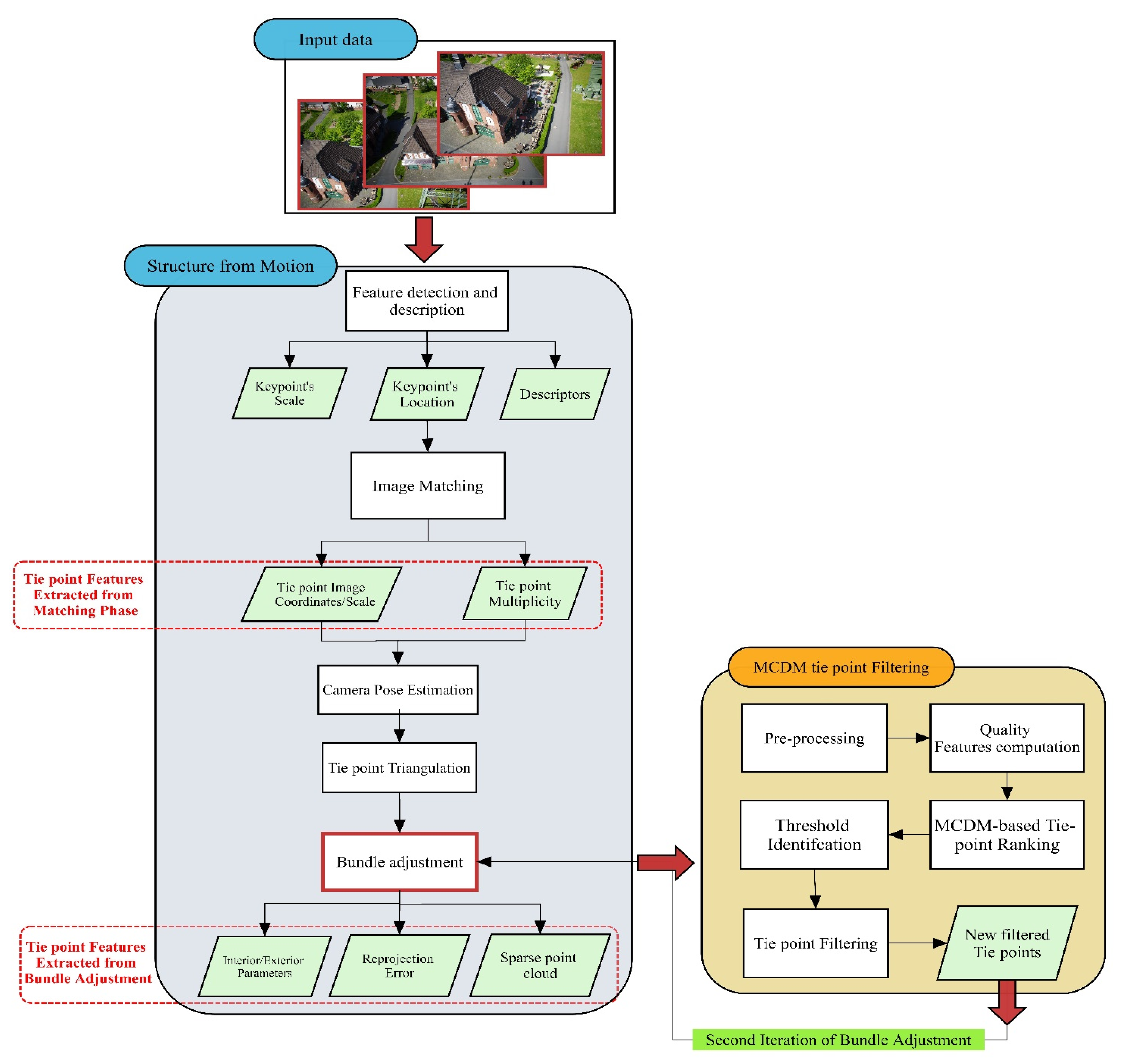
Figure 1 shows the workflow of the proposed algorithm. Given the initial camera calibrations parameters and exterior orientation parameters, the proposed strategy can be explained as follows:

(A)

Keypoints are extracted from images and matched to generate the initial tie points.

(B)

An initial bundle adjustment is conducted to compute interior/exterior camera parameters and sparse point cloud.

(C)

Tie points quality parameters are computed based on the matching results and the sparse point cloud.

(D)

A pre-processing stage is performed to remove grossly erroneous tie points.

(E)

A competency score is generated by aggregation of quality criteria using the MCDM method.

(F)

A statistical analysis is performed on the computed quality parameters to identify a suitable filtering threshold ($C_M$) for each dataset.

(G)

3D tie points with competency scores lower than the computed threshold are filtered out to develop a new set of tie points.

(H)

A new bundle adjustment is conducted to obtain refined camera parameters and a more accurate sparse point cloud.

3.2.2. Pre-Processing

Since the tie points are usually extracted automatically, some mismatches may occur, which lead to grossly erroneous tie points. We find and eliminate these points through a pre-processing stage. Given the re-projection error for each tie point on each of its visible images, the average re-projection error and standard deviation are calculated first. Standard deviation is calculated to eliminate erroneous keypoint matches which could not be detected by the average re-projection error. A smaller standard deviation represents the stability of tie points. Hence, when the average re-projection errors of two tie points are similar, the tie point with a larger standard deviation is considered as less accurate. A threshold is defined to eliminate the tie points with a large re-projection error which is defined as follows:

$$\mathsf{\alpha }= \overline{\mathsf{\mu }} +2\mathsf{\sigma }$$

(5)

where $\overline{\mu }$ and σ denote the average re-projection error and the standard deviation of the ith tie point, respectively.

3.2.3. MCDM-Based Tie Point Selection

Once the quality parameters are calculated and wrong tie points are removed, a competency score is computed by aggregation of the quality criteria and it is considered as an indicator to filter out the low-quality ones. Our proposed filtering strategy uses the MCDM techniques to compute the competency score of each tie point. A wide range of MCDM algorithms can be used. Our solution is general in this regard, as it does not depend on the type of the applied MCDM method and can easily work with all MCDM algorithms of different properties. The computational details of the MCDM method are explained in the following.

Definition of Decision Matrix

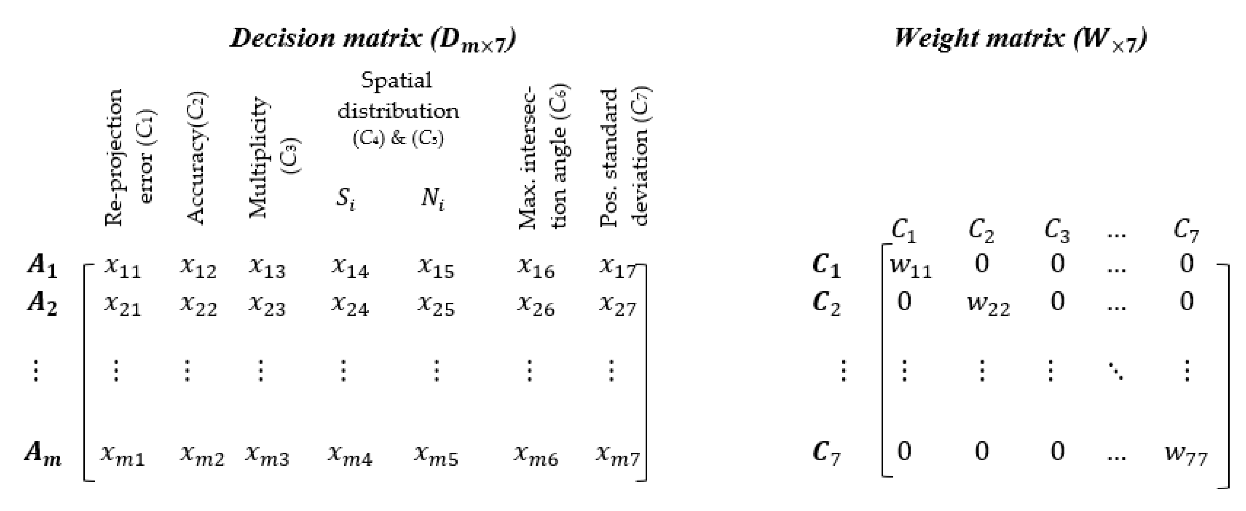
The applied MCDM problem is characterized by a set of m alternatives (tie points), denoted as $\left\{A_i| i=1,2,3,\cdots ,m\right\}$, that are evaluated according to the aforementioned quality criteria (Section 3.1), represented as $\left\{C_j| j=1,2,3,\cdots ,7\right\}$. These quality criteria can be regarded as a benefit or a cost in order to make decisions. A benefit criterion should be maximized, which means that the higher scores of an alternative (tie point) in terms of this criterion are better; on the other hand, lower values are preferred for cost criteria [31].

Additionally, each criterion is weighted, indicating its relative importance. These weights can be denoted as $W=\left\{w_j| j=1,2,3,\cdots ,7\right\}$ and they are usually normalized, so that their sum is equal to one: $\sum _{j=1}^7{w}_j=1$[32]. Thus, according to the Figure 2, the problem of selecting tie points using the MCDM technique can be concisely expressed as a matrix, where rows denoting the alternatives (initial tie points) and columns denote the selection criteria. Each element$x_{ij}$ of the decision matrix ($D_{m\times 7}$) represents the score of each alternative (tie point or $A_i$) with respect to the criterion$C_j$.

The objective of the proposed tie point filtering method is to rank the tie point alternatives according to their overall performance value which will be obtained by combining their quality scores and weights [33]. In our tie point filtering method, any MCDM method could be considered and applied to the decision problem to select an adequate subset of tie points. However, to precisely explain our method, a well-known and widely used MCDM algorithm, so-called TOPSIS (Technique for Order of Preference by Similarity to an Ideal Solution) [34] is selected and described.

MCDM Tie Point Ranking

The ranking process involves generating two matrices: the decision matrix ($D_{m\times 7})$and the weighting matrix ($W_{7\times 7}$). Using these, the TOPSIS method is used to rank the tie points. TOPSIS creates two sets of ideal and anti-ideal choices and prioritizes the possibilities based on the least distance from the ideal alternatives and the maximum distance from the anti-ideal alternatives. The ideal alternative maximizes profitability measures while minimizing cost criteria, whereas the anti-ideal option increases cost criteria minimizing profitability measures. TOPSIS method consists of the following steps:

A.

Decision matrix$D_{m\times 7}$ is normalized using the following equation:

$$r_{ij}=\frac{x_{ij}}{\sqrt{{\sum }_{i=1}^m{x}_{ij}^2}}$$

(6)

B.

The weighted normalized decision-making matrix is calculated:

$$V_{m\times 7}=D_{m\times 7} · W_{7\times 7}=\left[\begin{array}{ccc}{v}_{12}& \cdots & v_{17}\\ ⋮& \ddots & ⋮\\ v_{m1}& \cdots & v_{m7}\end{array}\right]$$

(7)

C.

The positive ideal solution ($V_j^{+}$) and negative ideal solutions ($V_j^{-}$) are determined using the following equations:

$$A^{+}=\left\{\left(max v_{ij}|j\in J\right),\left(min v_{ij}|j\in J\prime \right) \forall i=1,2,\dots ,m\right\}=\left\{v_1^{+},v_2^{+},\dots ,v_7^{+}\right\}$$

(8)

$$A^{-}=\left\{\left(min v_{ij}|j\in J\right),\left(max v_{ij}|j\in J\prime \right) \forall i=1,2,\dots ,m\right\}=\left\{v_1^{-},v_2^{-},\dots ,v_7^{-}\right\}$$

(9)

In which $J$ are positive criteria and $J\prime$ are negative ones.

D.

The separation measures from the positive ideal solution and the negative ideal solution are computed as follows:

$$s_i^{+}=\sqrt{{\displaystyle \sum }_{j=1}^7{\left(v_{ij}-v_j^{+}\right)}^2}$$

(10)

$$s_i^{-}=\sqrt{{\displaystyle \sum }_{j=1}^7{\left(v_{ij}-v_j^{-}\right)}^2}$$

(11)

E.

The closeness of relative Euclidean distance to the ideal solution is calculated by Equation (12) as follows:

$$C{l}_i^{*}=\frac{S_i^{-}}{S_i^{-}+S_i^{+}}\hspace{1em}\hspace{1em}0<C{l}_i^{*}<1$$

(12)

Finally, the $C{l}_i^{*}$ is considered as the competency score of each tie point. Therefore, tie points with higher values of $C{l}_i^{*}$, will have a higher rank.

3.3. Filtering Threshold Identification

Having computed the competency score for each 3D tie point, establishing appropriate thresholds for retaining only high-quality 3D points is challenging. The primary reason is the complexity of identifying an optimal threshold which is applicable to all types of datasets and image blocks. In our solution, we used the statistical distribution of each quality parameter to automatically determine a general threshold for the filtering process.

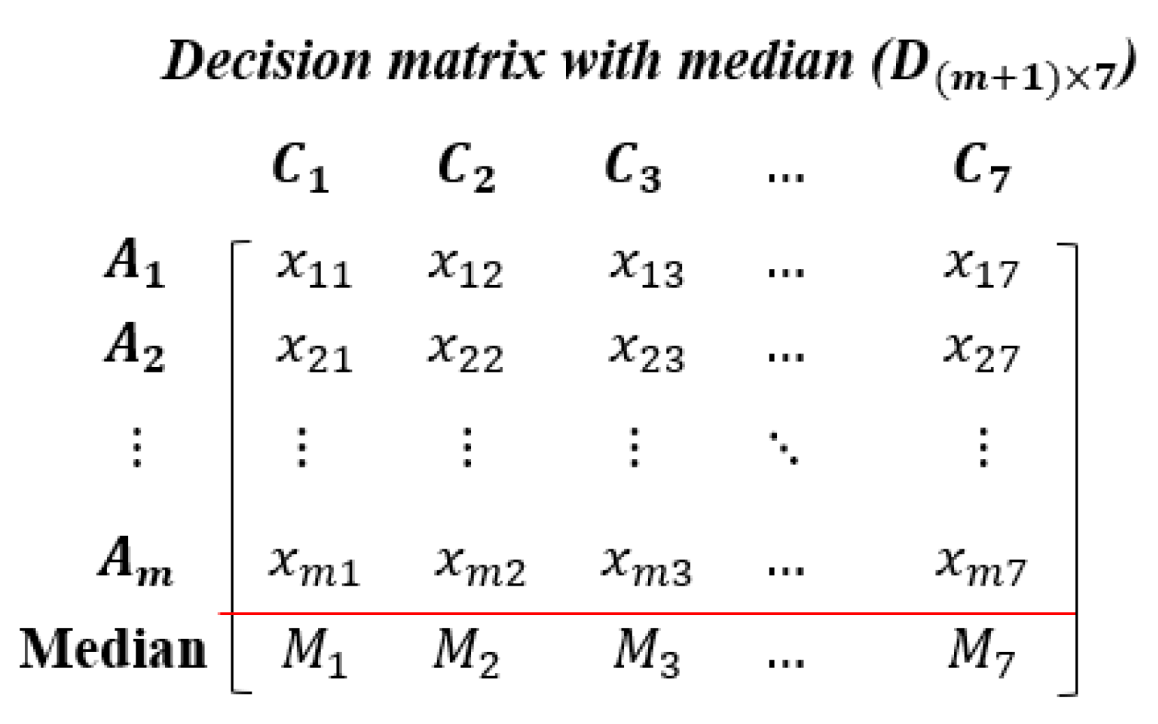
The concept underlying statistical distribution analysis of quality parameters is its resistance to outliers and improperly computed tie points. In our method, the median of each quality parameter is set as a new alternative and ranked using the MCDM algorithm. This technique proposes a robust method for threshold extraction because the median value of quality parameters is unaffected by outliers. In addition, in our filtering threshold identification method, the number of filtered tie points primarily depends on the initial number of tie points, the numerical range changes in each quality metric and the type of MCDM method used and it adaptively works in different blocks with different properties. The following steps are carried out:

A.

The median values of each quality parameter for all tie points are computed using the following equation:

$$M_i ; \forall i=1 to 7 \to M_i=Median\left(x_{1i},x_{2i},x_{3i},\cdots x_{mi}\right)$$

(13)

B.

The computed median values are inserted into the Decision Matrix as a new alternative, as shown in Figure 3.

C.

The MCDM algorithm is applied to compute a competency score for all tie points, and also the new alternative ($C_M$).

D.

Finally, the computed competency score of the new alternative ($C_M$) is considered as the filtering threshold. So, the tie points with competency scores lower than $C_M$ should be omitted.

4. Results

In this section, performance of the proposed methodology is evaluated. Concerning the first step of data quality evaluation, the results of the proposed filtering method using the TOPSIS algorithm are analysed and compared to the original (no filtering) results and the recent Farella algorithm, as presented in Section 4.4. Moreover, since our proposed filtering algorithm is supported by MCDM methods, a thorough evaluation of how different MCDM methods may affect the selected tie points is provided. These results could provide specific guidance for selecting the most appropriate approach to be used when dealing with tie point filtering problem. Therefore, an evaluation test (Section 4.5) is conducted with other MCDM methods to investigate their effectiveness on the final results. In the following section, first, the mathematical details of other MCDM methods such as VlseKriterijumska Optimizacija I Kompromisno Resenje (VIKOR), Simple Additive Weighting (SAW) and COPRAS algorithms (Section 4.1) will be discussed. Then the quality measures used to evaluate the results and the applied datasets are explained in Section 4.2 and Section 4.3, respectively.

4.1. Other MDCM Techniques Used in Our Evaluations

This section explains the details of VIKOR, SAW and COPRAS methods used for comparison. These algorithms are among the most well-known/widely used methods applied in different fields in the literature.

4.1.1. SAW Method

Simple Additive Weighting (SAW) [35] is one of the most widely used methods to solve multi-attribute decision problems. The usefulness of the SAW method’s basic concept is finding the number of weighted performance ratings for each alternative on all attributes [36]. The highest score will be the best alternative. SAW requires a process of normalizing the decision matrix ($D_{m\times 7}$) according to the following formula. Equation (14) is used if j is an attribute of benefit, and Equation (15) is used if attribute j is cost.

$$r_{ij}=\frac{x_{ij}}{max{x}_{ij}} i=1,2,3,\dots ,m j=1,2,\dots ,7$$

(14)

$$r_{ij}=\frac{min{x}_{ij}}{x_{ij}} i=1,2,3,\dots ,m j=1,2,\dots ,7$$

(15)

The preference value for each alternative ($V_i$) is given as:

$$V_i={\displaystyle \sum }_{j=1}^7{w}_j{r}_{ij} i=1,2,3,\dots ,m$$

(16)

4.1.2. VIKOR Method

The VIKOR (VlseKriterijumska Optimizacija I Kompromisno Resenje) method [37], similar to the TOPSIS, is based on distance measurements. In this approach, each alternative is evaluated according to all considered criteria and the compromise ranking is performed by comparing the measure of closeness to the ideal alternative. However, VIKOR differs in operational approach and the considered method for the concept of proximity to the ideal solutions. The steps of VIKOR algorithm are as follows:

A.

The normalized decision-making matrix ($D_{m\times 7}$) is calculated similarly to the TOPSIS method.

B.

The best $f_j^{*}$ and the worth $f_j^{-}$ values for all criteria functions $j=1,2,\dots ,7$ are determined. Equation (17) is used for benefit criteria, and Equation (18) is used for cost ones as follows:

$$f_j^{*}=max{x}_{ij} . f_j^{-}=min{x}_{ij} j=1,2,\dots ,7$$

(17)

$$f_j^{*}=min{x}_{ij} . f_j^{-}=max{x}_{ij} j=1,2,\dots ,7$$

(18)

C.

The $S_i$ and $R_i$values are calculated by following Equations.

$$S_i={\displaystyle \sum }_{j=1}^7{w}_j\left(f_j^{*}-x_{ij}\right) / \left(f_j^{*}-f_j^{-}\right)$$

(19)

$$R_i=max\left[w_j\left(f_j^{*}-x_{ij}\right) / \left(f_j^{*}-f_j^{-}\right)\right]$$

(20)

where$w_j$ are the weights of criteria, expressing their relative importance.

D.

The values $Q_i;i=1,2,3,\dots ,m$are computed by the following equation.

$$Q_i=\vartheta \left(S_i-S^{*}\right)/\left(S^{-}-S^{*}\right)+\left(1-\vartheta \right)\left(R_i-R^{*}\right)/\left(R^{-}-R^{*}\right)$$

(21)

where $S^{*}=\min S_i. S^{-}=\max S_i$and $R^{*}=\min R_i. R^{-}=\max R_i$. $\vartheta$ is introduced as weight of the strategy of ‘‘the majority of criteria”, in our implementation, we consider $\vartheta$ = 0.5.

E.

Alternatives (tie points) are ranked by sorting by the values of Q in ascending order.

4.1.3. COPRAS Method

COPRAS (Complex Proportional Assessment), introduced by Zavadskas et al. [38] assumes a direct and proportional relationship of the ideal solution to the ratio of the anti-ideal solution. This method ranks alternatives based on their relative importance (weight), and the final ranking is created using the positive and negative ideal solutions. Assuming the decision matrix ($D_{m\times 7}$), the COPRAS method is defined in the following steps:

A.

Decision matrix ($D_{m\times 7}$) is formed and normalized. The weighted normalized decision-making matrix is calculated using Equation (7).

B.

Sums of weighted normalized values are determined using Equation (22) for profit criteria and Equation (23) for cost criteria:

$$S_{+i}={\displaystyle \sum }_{j=1}^k{v}_{ij}$$

(22)

$$S_{-i}={\displaystyle \sum }_{j=k+1}^7{v}_{ij}$$

(23)

where k is the number of profit/benefit criteria. The rest of criteria from k+1 to 7 are the number of cost criteria. The $S_{+i}$ and $S_{-i}$ values show the level of the goal achievement for alternatives. A higher value for $S_{+i}$ and also lower value for $S_{-i}$ points to better alternatives.

C.

Calculate the relative significance of alternatives using the following Equation:

$$Q_i=S_{+i}+\frac{S_{-min}{\sum }_{i=1}^m{S}_{-i}}{S_{-i}{\sum }_{i=1}^m\left(\frac{S_{-min}}{S_{-i}}\right)}$$

(24)

$$S_{-min}=min S_{-i} i=1,2,\dots ,m$$

(25)

D.

Final ranking is performed according to the $U_i$ values computed as follows:

$$U_i=\frac{Q_i}{Q_i^{max}}·100\%$$

(26)

where $Q_i^{max}$is the maximum value of the relative significance of alternatives. Alternatives (tie points) with higher values of $U_i$ will have a higher rank.

4.2. The Quality Criteria Used for Comparisons

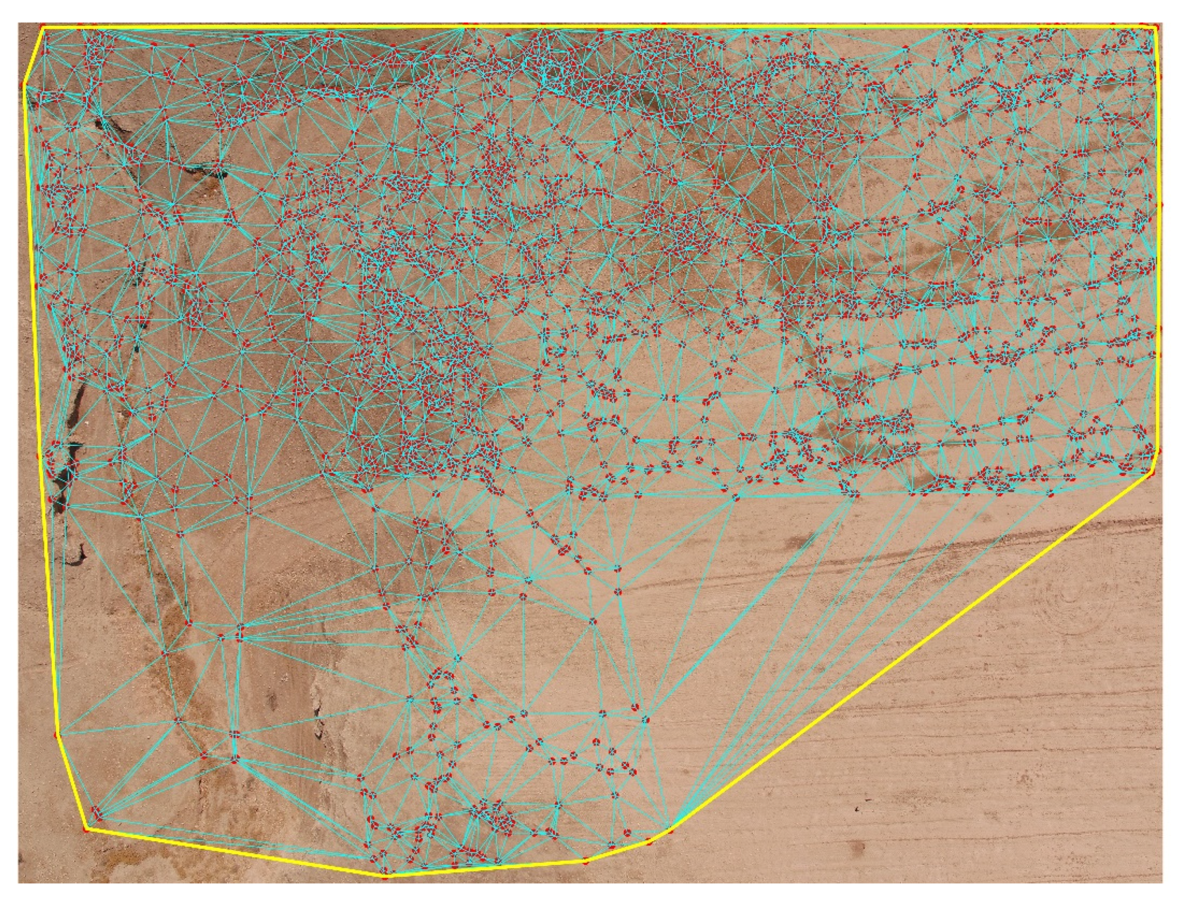
To evaluate the quality of the selected tie points, internal statistics can be used. To this end, median, mean and standard deviation values for the quality parameters are computed for each tie point in the first evaluation phase. To evaluate the distribution quality, the global coverage index α (Figure 4), which is based on Delaunay triangulations is computed by:

$$\alpha =\frac{{\sum }_{i=1}^n{A}_i}{A_{Total}}$$

(27)

where $A_i$ is the area of the ith triangle, n is the number of triangles and $A_{Total}$ is the area of the whole image. In the index (α), all points in the image are triangulated through the Delaunay triangulations. The numerator of α is equal to the area of the triangles covering all the computed tie points of the image. While its denominator shows the total area of the image. The larger the α value, the better the spatial distribution of the tie points. Since the (α) value is computed for each single image in the block, the computed values are different for each image, therefore, the median, mean and STD values are reported to measure its changes and difference in each image of the block.

Furthermore, external quality checks using 3D ground truth (GCPs) data are used to evaluate the image orientation results and possible block deformations. The planimetric ($E_{pl}$) and altimetric ($E_{Al}$) Euclidean distance and Root Mean Square Error (RMSE) of the checkpoints $(x_{ch},y_{ch},z_{ch})$measured points $(x_m,y_m,z_m)$are computed in order to assess the errors as follows: (N indicates the number of GCPs)

$$E_{pl}=\frac{{\sum }_{i=1}^N\sqrt{{\left(x_m-x_{ch}\right)}^2+{\left(y_m-y_{ch}\right)}^2}}{N}$$

(28)

$$E_{Al}=\frac{{\sum }_{i=1}^N\left(abs\left(z_m-z_{ch}\right)\right)}{N}$$

(29)

$$RMS{E}_x=\sqrt{\frac{1}{N}\sum _{i=1}^N{\left(x_m-x_{ch}\right)}^2}$$

(30)

$$RMS{E}_y=\sqrt{\frac{1}{N}\sum _{i=1}^N{\left(y_m-y_{ch}\right)}^2}$$

(31)

$$RMS{E}_z=\sqrt{\frac{1}{N}\sum _{i=1}^N{\left(z_m-z_{ch}\right)}^2}$$

(32)

As another external quality check, geometric accuracy and surface deviation of the newly generated dense point cloud are also evaluated. The geometric accuracy of our generated dense cloud is evaluated through cloud-to-cloud (C2C) comparisons. To this end, the dense cloud obtained from the original processing and the one produced after the filtering step were compared with the reference laser scanning data.

The surface deviation analysis process is performed based on defining a fitted plane on some selected areas using Least Squares Fitting (LSF) algorithm [39]. Similar to the [40] analysis, the C2C distance and spatial distribution of the points around the best-fitted plane are measured using well-known error metrics such as Standard Deviation (STD), Mean Absolute Error (MAE) and RMSE according to the following Equations:

$$STD=\sqrt{\frac{1}{M-1}{\displaystyle \sum }_{i=1}^M{\left(D_i-\overline{D}\right)}^2}$$

(33)

$$RMSE=\sqrt{\frac{1}{M}{\displaystyle \sum }_{i=1}^M{\left(D_i\right)}^2}$$

(34)

$$MAE=\sqrt{\frac{1}{M}{\displaystyle \sum }_{i=1}^M\left|D_i\right|}$$

(35)

which M defines as the number of observed data points of the sample, $D_i$ is the distance value of each point to the corresponding reference point or surface, $\overline{D}$ is the average value of the distance.

4.3. Description of Datasets

Performance evaluation of our algorithm was carried out on different image networks with different properties to check the effectiveness of our method in different blocks. The applied datasets are characterized by different image resolutions, number of images, image overlap, illumination changes and surfaces with different textures and sizes. Furthermore, we aimed to consider different types of UAV image networks, including normal UAV networks, hybrid networks with horizontal and vertical images, joint networks containing both terrestrial and UAV images and close-range networks with convergent UAV images. Thereafter, four datasets were used to cover all network geometries and analyse the results of our algorithm in different situations. The specifications of each dataset are explained as follows:

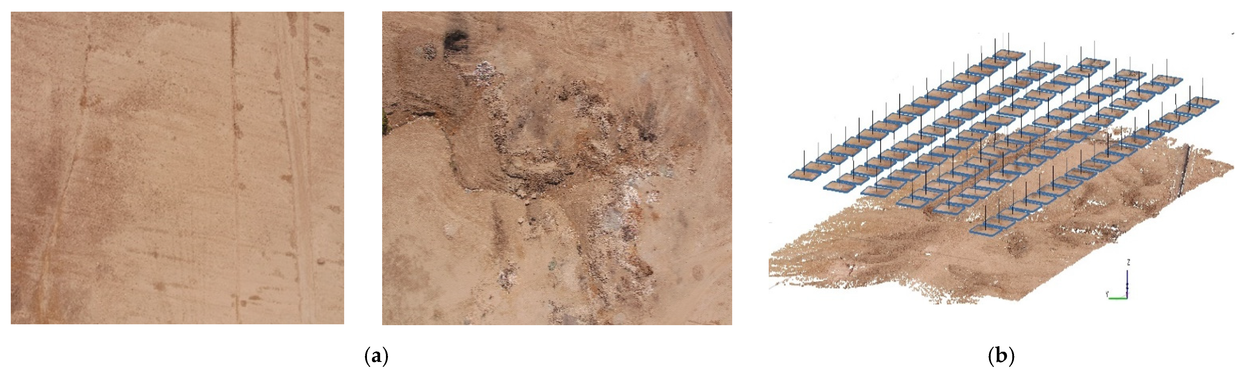
• Normal UAV image network: The Dezful dataset is surveyed using 100 UAV images captured using a conventional image network with an average image overlap of 60% and GSD of 2.86 cm/pix. The survey was conducted at the region without great topographic relief by a low-cost aircraft equipped with a DJI FC6520 camera with the focal length of 12 mm and pixel size of 3.2 µm. The images cover a soil-type area with mostly texture-less surfaces, potentially causing feature matches to accumulate in a small region of the image. Therefore, this experiment determines whether our proposed algorithm is capable of selecting a subset of high-quality tie points or not. Figure 5a shows sample images of the dataset, and Figure 5b shows the network geometry.

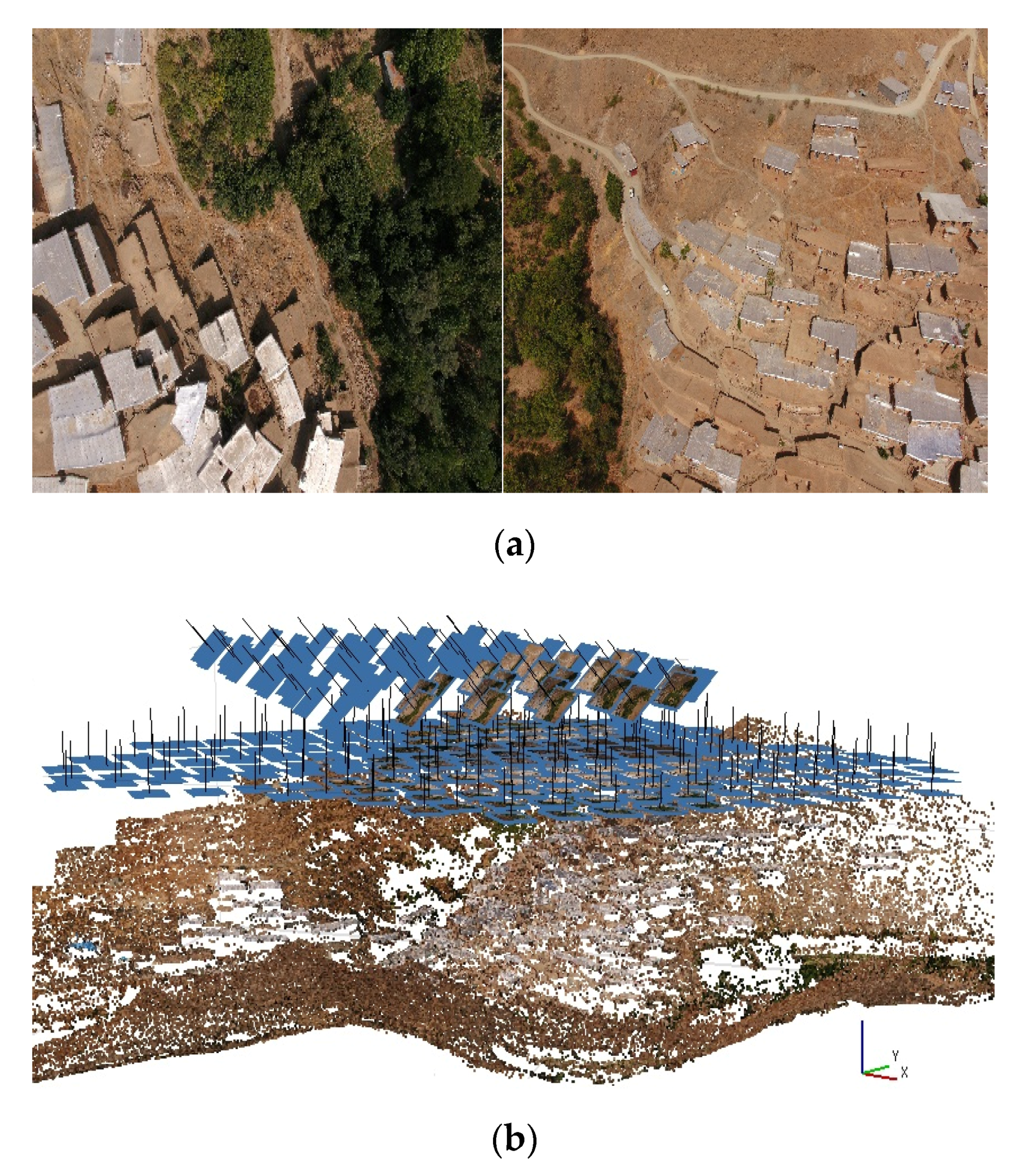
• Hybrid horizontal and vertical image network: The Halavan dataset contains 238 UAV images with an average GSD of 2.81 cm/pix. These images were captured from the village of Halavan in a mountainous region using a DJI Inspire2 UAV camera (12 mm focal length) with an imaging network containing both horizontal and semi-vertical images. The village has a stepped form architecture, with tall trees and semi-glossy roofs of buildings. These objects cover a large area of images and present a complicated situation where few keypoints are extracted, and the accuracy of aerial triangulation is degraded. Therefore, the presence of this experiment demonstrates whether the proposed algorithm is capable of detecting and filtering these keypoint or not. Figure 6a shows some sample images of the dataset, and Figure 6b shows the imaging network geometry.

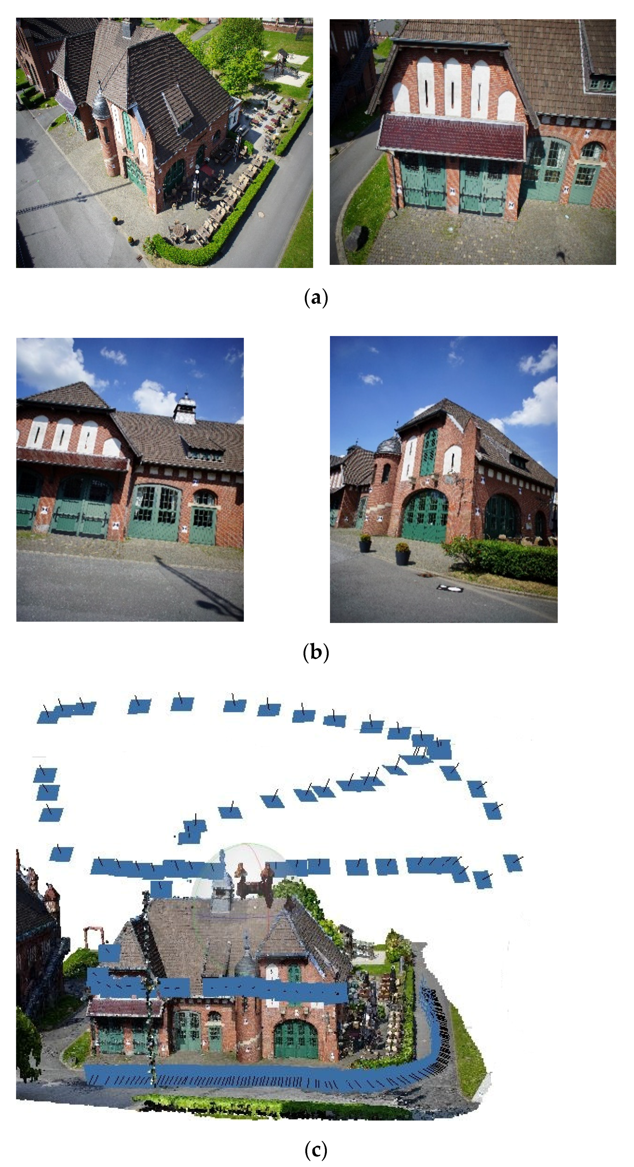
• Hybrid terrestrial and UAV image network: In ISPRS Dortmund Benchmark [41], the area of Zeche Zollern was surveyed using UAV, terrestrial images as well as Terrestrial Laser Scanner (TLS). Our experiments selected a joint UAV and terrestrial image network of Pferdestall building. The dataset contains 126 terrestrial images (average GSD of 3 mm) and 97 UAV images (average GSD of 2 cm) captured by a NEX-7 camera with a 16 mm lens and 4µm pixel size. The building is also surveyed with high-quality scans of the objects with a Z+F 5010C laser scanner. Sample images of UAV-based and terrestrial images are shown in Figure 6a and Figure 7b, and the imaging network geometry is shown in Figure 7c.

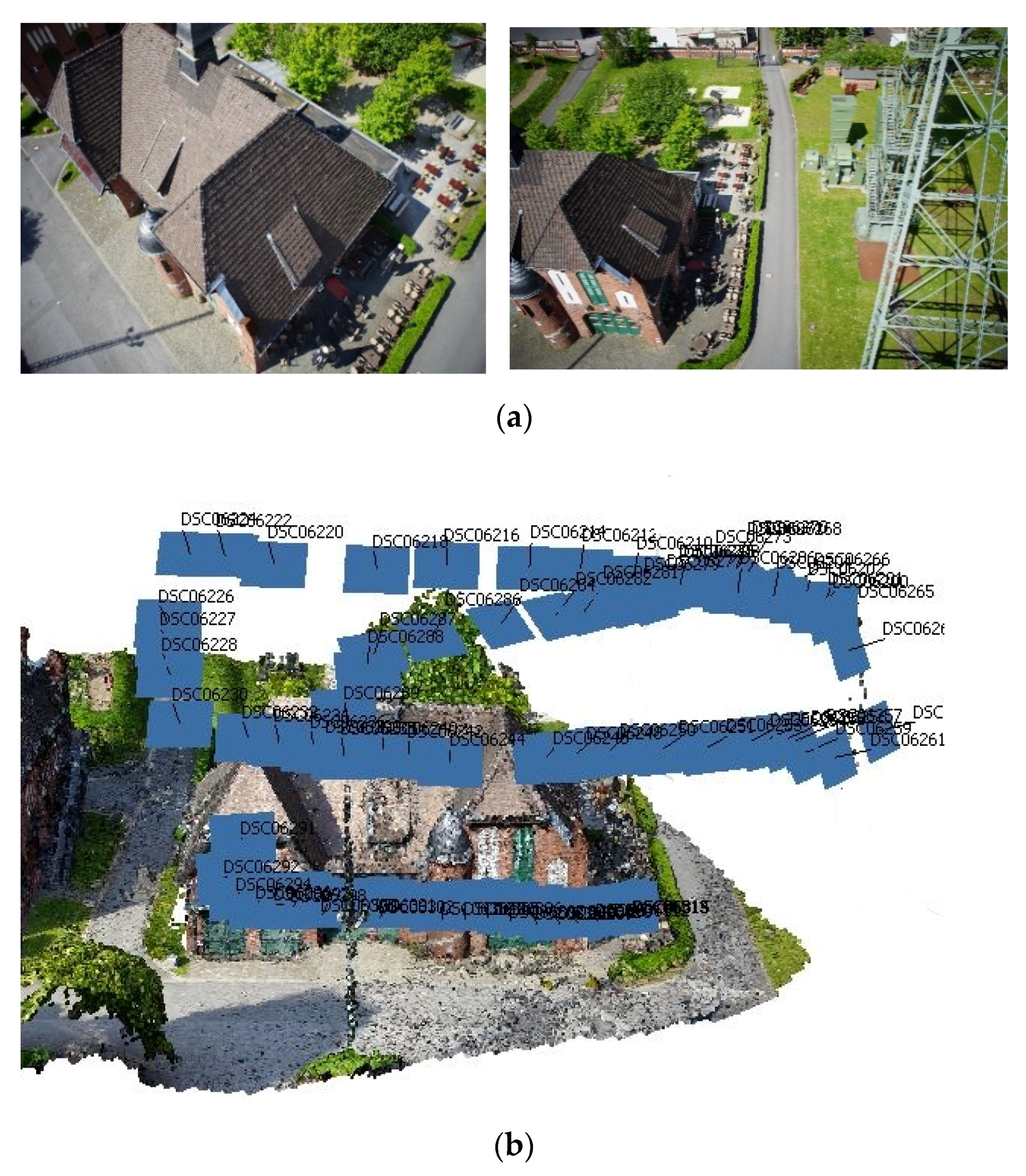
• UAV Convergent image network: A small part of the Dortmund benchmark with a low altitude convergent image network was considered in this dataset. It contains 97 UAV images, with average overlapping of 88% and an average GSD of 2 cm, captured by a NEX-7 camera. Figure 8a shows some sample images of the dataset, and Figure 8b shows the geometry of the imaging network.

4.4. Experimental Results of the MCDM Filtering Method

In the following sections, the results using the TOPSIS algorithm of different UAV block case studies are provided to show the effectiveness and capabilities of the proposed methodology. To produce these results, initial tie points were extracted from Agisoft software. The filtering pipeline, including the quality measure computations and MCDM methods, were implemented in MATLAB (R2018b), and the open-source DBAT toolbox [42] was used to run the photogrammetric bundle adjustment. In all our experiments, the weighting matrix is considered as an identity matrix to avoid unknown and unstudied complexity to our method, since the relative importance of the criteria is not clear. To implement the Farella method, the provided python source code [43] is used, which is automatically performed on initial tie points. In this tool, the user is not required to set any parameters. In the following, the results of each test on different UAV photogrammetry blocks are shown and discussed.

4.4.1. Results of Dezful Dataset

From the orientation results of Dezful images in Agisoft software, about 353,715 tie points were derived in the sparse point cloud. After applying the Farella filtering algorithm, a new set of 3D tie points of about 213,505 were returned, which indicates about 40% of the original sparse cloud is removed. Once a suitable threshold was identified in our filtering method, 211,254 tie points were selected, indicating an almost similar reduction. The quality features median, mean and standard deviation values computed on the original sparse point cloud, the Farella filtering and our proposed algorithm are presented in

Table 1. Calculated median, mean and STD values for the quality features of the Dezful dataset.

	No Filtering			Farella Method			Proposed Method
	Median	Mean	STD	Median	Mean	STD	Median	Mean	STD
Re-projection error (pix)	0.573	0.567	0.142	1.273	1.480	0.873	0.409	0.417	0.099
Multiplicity	2.365	2.000	0.821	2.431	2.000	0.838	2.718	2.000	0.983
Spatial Distribution (α) (%)	98.524	98.762	1.171	78.120	78.683	2.420	96.420	96.698	1.535
Maximum intersection angle (deg)	23.474	28.616	10.878	23.150	28.233	10.729	34.652	33.596	12.001
Pos. standard deviation (mm)	29.63	32.87	35.34	45.94	53.20	42.71	24.03	26.17	11.09
Number of returned tie-points	353,715			213,505			211,254

. The results show that in our proposed method, all quality metrics have been improved compared to the original and the Farella filtering method. With respect to the original results, our method’s median and mean improvements are about 28%, 15%, 47% and 18% for re-projection error, multiplicity, maximum intersection angle and posterior standard deviation quality measures, respectively. These values are about 66%, 11%, 49% and 47% compared to the Farella filtering method. The spatial distribution metric confirms the capability of our method to select well-distributed tie points. Despite of tie point elimination, the distribution of the selected tie points in our filtering strategy is not degraded compared to the original one.

To further evaluate the improvements in external quality, the Euclidean distance and RMSEs on 7 checkpoints were measured. The average multiplicity of check points was 4.14 in this dataset.

Table 2. Checkpoint RMSEs in the Dezful dataset.

	RMSE (pix)	RMSE(x) (cm)	RMSE(y) (cm)	RMSE(Al) (cm)	E(Pl) (cm)	E(Al) (cm)
No filtering	0.7110	15.0270	32.2000	43.8300	33.4200	33.2700
Farella Method	0.5759	9.3313	22.4959	24.0668	26.1200	19.4038
Proposed Method	0.4823	3.8700	7.6500	18.6000	10.0571	14.5429

compares the average improvement by our procedure against those of the original one and also Farella method. As it shows, the RMSE of checkpoints for Farella algorithm was improved 19% in image space and about 37%, 30% and 56% in the X, Y and Z dimensions, respectively. These amounts were calculated as 32% in image space and 75%, 76% and 57.5% for our algorithm. For the planimetric and altimetric errors, the results indicated an average 21% and 41% improvement in Farella results, while our method has superior results with 70% and 56% of accuracy increase.

4.4.2. Results of Halavan Dataset

About 230,656 tie points were extracted from the image orientation results in Agisoft software. The Farella filtering algorithm returned a new set of 79,137 tie points which shows a reduction of about 65%. However, our filtering method reduced nearly 30% of the initial tie points and returned a new set of 162,343 tie points.

Calculated median, mean and standard deviation values for the quality measures are summarized in

Table 3. Calculated median, mean and STD values for the quality features of the Halavan dataset.

	No Filtering			Farella Method			Proposed Method
	Median	Mean	STD	Median	Mean	STD	Median	Mean	STD
Re-projection error (pix)	1.496	1.526	1.609	1.974	1.928	1.897	1.249	1.325	0.607
Multiplicity	2.000	3.070	2.284	2.000	3.066	2.257	3.000	3.514	2.595
Spatial Distribution (α) (%)	98.527	98.747	2.039	71.867	71.618	3.328	98.473	98.728	2.232
Maximum intersection angle (deg)	16.900	20.587	12.260	16.840	20.513	12.208	19.822	23.043	12.825
Pos. standard deviation (mm)	74.791	86.48	45.59	50.8725	48.421	59.356	14.320	23.574	15.510
Number of returned tie-points	230,656			79,137			162,343

for unfiltered sparse point cloud, the Farella algorithm and our method. As Table 3 shows, compared to the original results, an average median, mean and STD value improvement of (16%, 13%, 62%) for re-projection error, (50%, 14%, 13%) for multiplicity, (17%, 12%, 5%) for maximum intersection angle and (80%, 72%, 65%) for posterior standard deviation are achieved. Similarly, in comparison to the Farella algorithm, median and mean values in our method are significantly increased. These amounts are (36%, 31%) for re-projection error, (50%, 14%) for multiplicity, (17%, 12%) for maximum intersection angle and (71%, 51%) for posterior standard deviation. Additionally, the spatial distribution of our method is notably better than Farella method and is similar to the original one. These results indicate a higher performance of our algorithm in terms of inner quality metrics.

The RMSEs on 28 checkpoints (

Table 4. Checkpoint RMSEs in Halavan dataset.

	RMSE (pix)	RMSE(x) (cm)	RMSE(y) (cm)	RMSE(Al) (cm)	E(Pl) (cm)	E(Al) (cm)
No filtering	2.813	30.192	57.666	59.077	34.425	52.886
Farella Method	2.698	26.388	32.274	25.587	30.388	24.567
Proposed Method	1.888	7.161	8.243	5.440	9.914	4.171

) with average multiplicity of 31.3, were calculated to assess the external quality of our proposed filtering in comparison to the original and Farella methods. The results demonstrate that the RMSE of checkpoints has greatly decreased after the application of our filtering algorithm. This improvement is about 32% in image space and about 76%, 85% and 90% in the X, Y and Z dimensions, respectively. From the planimetric and altimetric points of view, our results indicate an average 71% and 92% improvement.

The Farella algorithm, on the other hand, does not perform as well as ours, with a 4% improvement of RMSE in image space and about 12.5%, 44% and 56% in the X, Y and Z directions, respectively. Furthermore, their method achieves an average planimetric and altimetric improvement of 12% and 53%.

4.4.3. Results of ISPRS Dortmund Dataset

The processing of both UAV and terrestrial images in Agisoft software produced a sparse point cloud with 416,047 tie points. Adopting the Farella filtering algorithm, a new set of about 213,505 tie points was returned, which implies a 48.5% reduction in the original sparse cloud. In our filtering method, 211,254 tie points were selected, representing a nearly 49% elimination in the number of tie points. The results of the quality parameters extracted from the original and filtering methods are presented in

Table 5. Calculated median, mean and STD values for the quality features of the ISPRS Dortmund dataset.

	No Filtering			Farella Method			Proposed Method
	Median	Mean	STD	Median	Mean	STD	Median	Mean	STD
Re-projection error (pix)	1.919	1.950	1.885	1.548	1.123	1.649	1.335	1.250	1.885
Multiplicity	2.000	3.405	3.268	2.000	3.403	3.248	3.000	4.308	3.933
Spatial Distribution (α) (%)	94.087	91.992	5.435	89.510	85.015	8.817	92.988	90.378	6.223
Maximum intersection angle (deg)	4.578	8.028	9.981	4.560	7.995	9.948	7.376	11.332	11.534
Pos. standard deviation (mm)	16.42	24.41	29.10	16.47	19.75	21.11	12.03	18.63	16.61
Number of returned tie-points	416,047			117,989			253,191

. As it shows, compared to the original results, our filtering method enhances the median and means of quality metrics by an average of 30% and 35% for re-projection error, 50% and 26% for multiplicity, 58% and 41% for maximum intersection angle and 26% and 23% for posterior standard deviation. Our method’s spatial distribution is superior to that of Farella method and is close to the original result.

Two tests were performed as an external check in this dataset, including the evaluation of RMSEs on checkpoints and the comparison of the produced dense cloud to the reference TLS point cloud data.

Table 6. Checkpoint RMSEs in ISPRS Dortmund dataset.

	RMSE (pix)	RMSE (x) (cm)	RMSE (y) (cm)	RMSE (Al) (cm)	E (Pl) (cm)	E (Al) (cm)
No filtering	2.833	19.679	20.485	17.645	21.960	16.825
Farella Method	2.570	18.722	19.906	13.268	19.610	12.032
Proposed Method	2.216	16.632	17.313	6.461	15.936	5.250

shows the RMSEs on 20 checkpoints measured with the GNSS instrument. The average multiplicity of check points was 39.8 in this dataset. As it shows, the average improvement of RMSEs applying the Farella algorithm is 9% in image space and about 4%, 2% and 24%, in the X, Y and Z dimensions, respectively. In contrast, our method performs better with an average accuracy increase of 21% in image space and 15%, 15.5% and 63% for each direction.

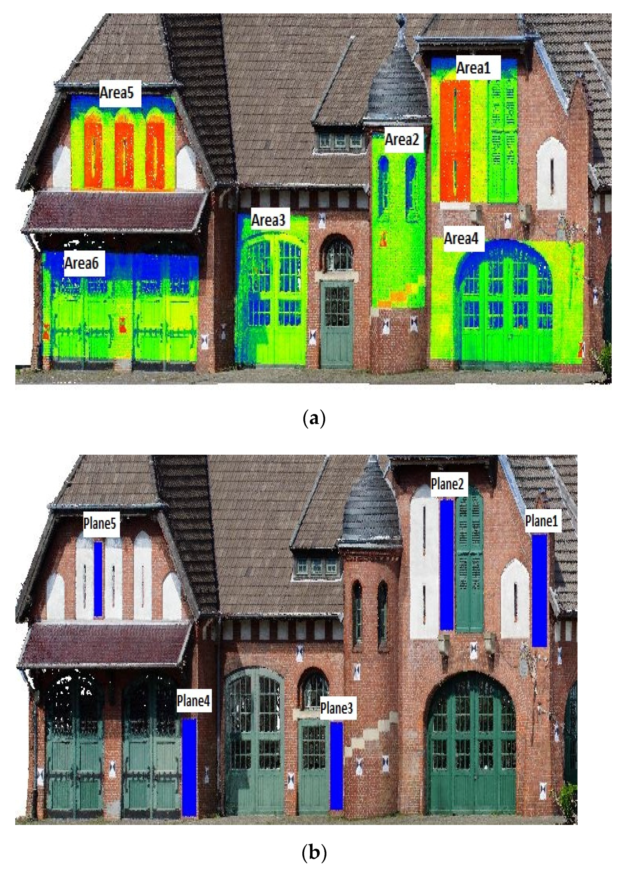
As the second test, the quality of the generated point clouds from the original method and those produced after the filtering step was compared using common quality evaluation methods, including surface deviation analysis and geometrical accuracy evaluations. To this end, at first, six sub-areas (Figure 9a) on the generated point clouds were selected, and the results of the cloud-to-cloud distance in these areas are compared to the reference TLS point cloud (

Table 7. Results of the cloud-to-cloud distance analyses on the original and filtered dense clouds in ISPRS Dortmund dataset.

Area	Original Dense Cloud		Farella Filtered Dense Cloud		Proposed Filtered Dense Cloud
	RMSE (mm)	Std. Dev. (mm)	RMSE (mm)	Std. Dev. (mm)	RMSE (mm)	Std. Dev. (mm)
AREA1	46.808	40.815	23.093	23.203	4.634	4.790
AREA2	32.398	25.777	23.633	23.782	10.490	18.314
AREA3	126.19	145.146	45.292	28.181	17.254	9.884
AREA4	15.303	21.721	12.023	9.072	12.335	7.831
AREA5	43.776	44.556	61.890	57.375	18.460	28.548
AREA6	38.807	28.548	28.771	24.220	6.662	5.353
Average	50.547	51.094	32.450	27.639	11.639	12.453

). Then, using five selected areas on dense cloud (Figure 9b), the plane fitting evaluations were conducted to measure the level of noise obtained for each method (

Table 8. Surface deviation analysis using the plane fitting in ISPRS Dortmund dataset, Unit: (mm).

Plane	Original Dense Cloud				Farella Filtered Dense Cloud				Proposed Filtered Dense Cloud
	MAE	STD	RMSE	Max Dist.	MAE	STD	RMSE	Max Dist.	MAE	STD	RMSE	Max Dist.
Plane1	29.207	20.873	35.899	99.468	18.014	17.639	25.212	394.25	5.390	4.416	6.968	30.424
Plane2	25.402	15.157	29.580	63.127	17.676	11.199	20.925	154.24	1.571	1.152	1.948	27.223
Plane3	16.820	12.353	20.868	69.457	17.130	15.939	23.398	97.840	1.359	8.385	15.974	41.370
Plane4	31.933	31.977	45.191	186.21	24.042	16.768	29.312	170.83	16.512	11.617	20.19	92.181
Plane5	36.244	25.248	44.171	121.77	24.902	19.166	31.424	113.78	1.815	1.688	2.479	15.535
Average	27.921	21.122	35.14	108.00	20.353	16.142	26.054	186.18	5.329	5.452	9.512	41.347

).

As shown in Table 7, the average standard deviation (STD) and the Root Mean Square Error (RMSE) for the original point cloud data were 50.54 mm and 51.09 mm, respectively. These amounts were calculated as 32.45 mm and 27.639 mm for the Farella filtered point cloud and also 11.63 mm and 12.45 mm for our method. These values indicated a greater performance using our filtering algorithm in terms of generating precise 3D models.

According to Table 8, the average results of the MAE, STD and RMSE for the original data set showed values greater than 21 mm, while these amounts were calculated as 20.35 mm, 16.142 mm and 26.054 mm for the Farella method, and 5.32, 5.45 and 9.512 mm for our proposed filtered point cloud, respectively. However, despite of improved performance of the Farella algorithm compared to the original results, the MAE, STD and RMSE obtained by their method are larger than those achieved by our methods. This indicates a higher noise level for both original and Farella algorithms, while our method’s noise level is smaller, showing a greater performance in terms of geometric accuracy of 3D models.

4.4.4. Results of ISPRS Pferdestall Convergent Dataset

Statistics computed on the extracted quality parameters of this dataset for the original and filtered sparse point clouds are given in

Table 9. Computed median, mean and standard deviation values for the quality features of ISPRS Pferdestall Convergent dataset.

	No Filtering			Farella Method			Proposed Method
	Median	Mean	STD	Median	Mean	STD	Median	Mean	STD
Re-projection error (pix)	1.560	1.826	1.311	1.517	1.665	1.379	1.335	1.286	0.211
Multiplicity	2.000	3.507	2.859	2.000	3.604	2.947	3.000	4.432	3.354
Spatial Distribution (α) (%)	98.331	98.603	0.769	97.02	97.35	0.897	97.913	98.418	2.051
Maximum intersection angle (deg)	5.463	9.309	10.533	5.539	9.430	10.721	8.919	12.725	11.802
Pos. standard deviation (mm)	29.36	28.10	24.63	20.25	24.42	20.57	13.25	12.35	18.75
Number of returned tie-points	181,597			62,276			119,932

. As it shows, processing the UAV images in Agisoft software produced 181,597 tie points. Using the Farella filtering algorithm, a new set of 62,276 tie points was returned, inferring a 60% reduction in the original sparse cloud. Our filtering method suggests a nearly 50% reduction, in which 119,932 tie points were selected.

An average median and mean value improvement of about (14%, 29%) for re-projection error, (50%, 26%) for multiplicity, (63%, 36%) for maximum intersection angle and (54%, 56%) for posterior standard deviation are achieved using our filtering algorithm. Furthermore, our method is superior to Farella method, with an average median improvement of 11% in re-projection error, 50% in multiplicity, 60% in maximum intersection angle and 34% in posterior standard deviation. Since higher overlapping images are captured in this dataset, the spatial distribution quality of filtering methods and the original one are almost similar. However, despite the elimination of tie points, the distribution of selected tie points in our filtering strategy is not weaker than the original.

Similar to the previous section, the RMSEs on check points and comparison to the reference TLS point cloud data are considered for the external check.

Table 10. Checkpoint RMSEs in ISPRS Pferdestall Convergent dataset.

	RMSE (pix)	RMSE (x) (cm)	RMSE (y) (cm)	RMSE (Al) (cm)	E (Pl) (cm)	E (Al) (cm)
No filtering	30.4302	10.6850	12.3916	24.4115	13.4211	27.4042
Farella Method	4.3457	5.1442	5.4742	9.5787	6.3747	6.6006
Proposed Method	1.3321	2.7532	2.3473	3.2726	1.6737	1.6474

shows the RMSEs computed on 19 checkpoints measured with the GNSS instrument. The average multiplicity of check points was 21 in this dataset. According to the results, the Farella algorithm improves RMSEs on image space by 85% and 51%, 55% and 60% in X, Y and Z directions in-ground space. Our method outperforms, with accuracy increases of 95% in image space and 74%, 81% and 82% in each direction. For the planimetric and altimetric errors, Farella results indicated an average of 52% and 75% improvement, whereas our method has superior results with an 87% and 94% increase in accuracy.

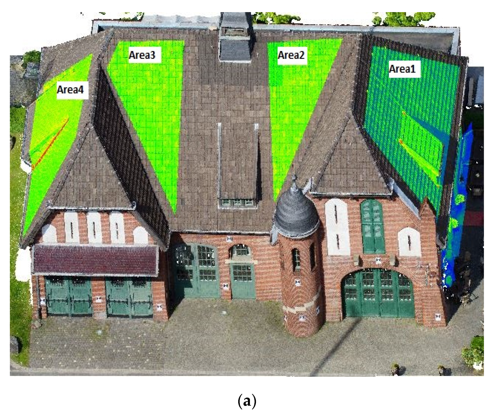
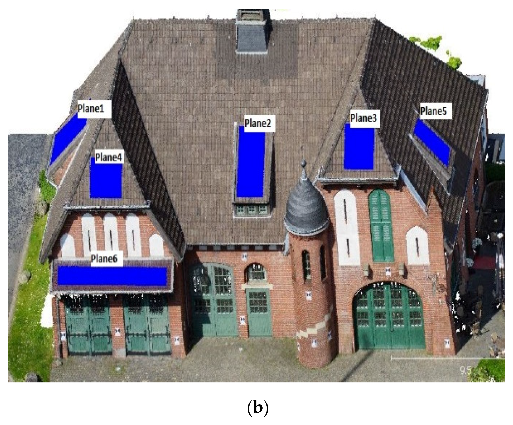
In addition, four sub-areas (Figure 10a) on the generated point clouds were selected, and the results of the cloud-to-cloud distance in these areas are computed. The average STD and RMSE of the original point cloud data, as shown in

Table 11. Results of the cloud-to-cloud distance analyses on the original and filtered dense clouds in the ISPRS Pferdestall Convergent dataset.

Area	Original Dense Cloud		Farella Filtered Dense Cloud		Proposed Filtered Dense Cloud
	RMSE (mm)	Std. Dev. (mm)	RMSE (mm)	Std. Dev. (mm)	RMSE (mm)	Std. Dev. (mm)
AREA1	57.13	44.502	47.401	65.259	8.3238	12.111
AREA2	26.644	20.767	35.671	33.222	12.047	6.605
AREA3	111.174	85.767	28.569	27.178	15.340	8.304
AREA4	30.566	39.617	23.039	24.819	19.096	17.200
Average	56.379	47.663	33.670	37.620	13.702	11.055

, were 56.37 mm and 47.66 mm, respectively. These values were calculated to be 33.67 mm and 37.62 mm for the filtered point cloud of Farella method and 13.702 mm and 11.055 mm for our method. These values indicated that our filtering algorithm performs effectively in generating accurate 3D models.

Furthermore, as shown in

Table 12. Surface deviation analysis using the plane fitting in ISPRS Pferdestall Convergent, Unit: (mm).

Plane	Original Dense Cloud				Farella Filtered Dense Cloud				Proposed Filtered Dense Cloud
	MAE	STD	RMSE	Max Dist.	MAE	STD	RMSE	Max Dist.	MAE	STD	RMSE	Max Dist.
Plane1	8.667	6.848	11.046	73.609	41.900	24.292	48.433	151.17	6.037	4.108	7.303	31.481
Plane2	44.968	33.612	56.142	804.47	16.241	14.352	21.674	91.726	7.427	4.978	8.941	26.745
Plane3	10.848	11.691	15.948	102.87	14.547	11.630	18.607	79.517	7.918	6.889	10.496	69.096
Plane4	7.369	7.748	10.692	103.44	4.908	4.530	6.679	76.662	5.873	4.744	7.479	60.081
Plane5	43.15	28.914	51.830	159.11	9.760	7.797	12.555	54.406	6.93	4.156	7.375	29.778
Plane6	40.341	35.558	53.775	447.62	41.333	24.347	47.971	459.77	3.655	2.992	4.723	49.837
Average	26.584	20.491	33.65	292.47	11.364	9.577	14.879	75.578	7.037	5.192	8.573	46.425

, the plane fitting analysis using six selected areas on dense cloud (Figure 10b), indicated an average MAE of 26.584 mm, STD of 20.491 mm and RMSE of 33.653 mm for the original point cloud data. Moreover, for the Farella filtering algorithm, the amount of MAE, STD and RMSE were calculated as 11.364 mm, 9.577 mm and 14.879 mm, respectively. However, our algorithm revealed a lower level of noise for the acquired dense point cloud with MAE, STD and RMSE of 7.037 mm, 5.192 mm and 8.573 mm, respectively.

4.5. Evaluating the Proposed Technique Using other MCDM Algorithms

In this section, some test has been performed to evaluate the influence of the MCDM method on the final filtering results. As experiments in previous sections have shown, our proposed method outperforms the original and the recent filtering method. However, since different MCDM methods can make different ranking results, it may result in either orientation failure due to inadequate tie points or incorrect orientation results. Therefore, the experiments in this section evaluate the impact of the MCDM methods, as discussed in Section 4.1 on the results of the filtering algorithm as follows.

4.5.1. Average Re-Projection Error of the Bundle Adjustment

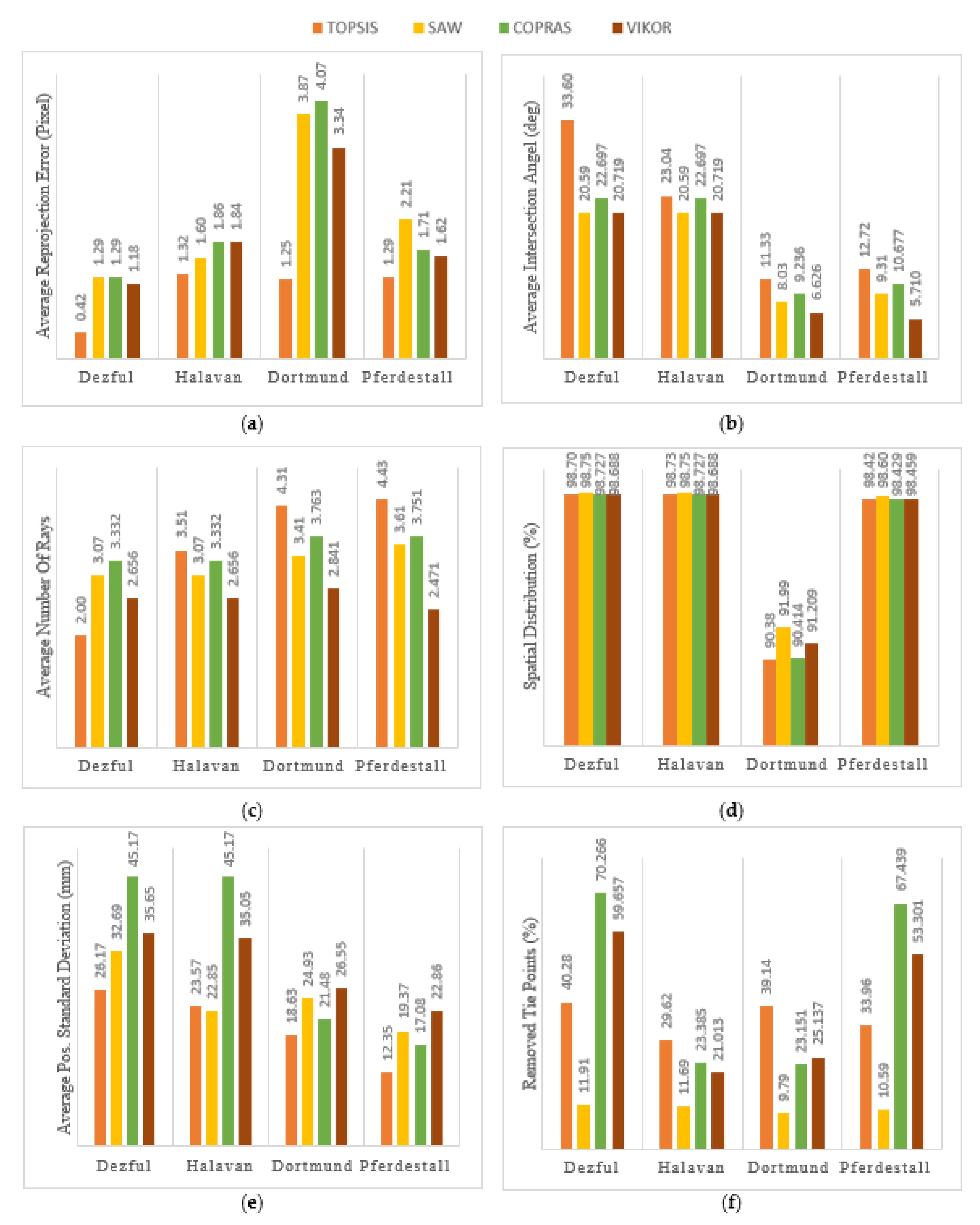
The re-projection error obtained using each MCDM method is shown in Figure 11a for all datasets. As shown, the TOPSIS algorithm performs better than the SAW, Complex Proportional Assessment (COPRAS) and VIKOR methods for all datasets. The re-projection error using the TOPSIS algorithm is averagely 25% to 66% lower compared to other MCDM methods. The SAW and COPRAS methods perform relatively weaker in terms of the re-projection error.

4.5.2. Average Angles of Intersection

To provide more accurate triangulation for 3D point calculation, a higher angle of intersection of similar rays is required. As shown in Figure 11b, the intersection angles in the TOPSIS algorithm are significantly higher. The intersection angles in the TOPSIS method are averagely 26% better than other methods. However, the average intersection angles are relatively smaller for Dortmund and Pferdestral datasets with higher overlapping images. SAW and VIKOR algorithms slightly perform weaker in terms of selecting tie points with larger intersection angles.

4.5.3. Average Multiplicity

As the number of images and their overlap increases in a dataset, larger multiplicities and thus more accurate 3D object coordinates are expected. As shown in Figure 11c, a higher average multiplicity for the selected tie points is achieved by the TOPSIS algorithm with an average of 2.56 rays. Nevertheless, for the Dezful dataset, the average multiplicity of the COPRAS algorithm is relatively higher, with 3.33 rays on averagely.

4.5.4. Average Spatial Distribution of Tie Points

The well-distributed tie points are crucial for accurate image orientation and 3D reconstruction. According to Figure 11d, the spatial distribution of selected tie points does not change significantly using MCDM methods. The average difference between different MCDM methods is around 1%, indicating that all applied MCDM methods can select well-distributed tie points. The main reason for having the spatial distribution of about 100% in almost all MCDM methods is that the resulting tie points are well distributed on the images. This shows that using the proposed method, we will have subsets of well-distributed tie points on the images.

4.5.5. Average Posteriori Standard Deviation of Object Coordinates

As Figure 11e shows, the average posteriori standard deviation of the 3D points for the TOPSIS algorithm with an average of 20.18 mm is the lowest in all datasets. For Dezful and Halavan datasets, COPRAS has the weakest performance with an average deviation of 45.17 mm; for the Dortmund and Pferdestall datasets, VIKOR has the lowest performance with a standard deviation of 24.70 mm.

4.5.6. The Percent of Removed Tie Points

Figure 11f shows the percent of eliminated tie points during the filtering process using different MCDM methods. As it shows, the number of removed tie points is different in MCDM methods. The TOPSIS and SAW algorithms averagely remove 35% and 11% of the initial tie points. In comparison, COPRAS and VIKOR remove mostly remove a larger number of points of about 70% and 56% of tie points in Dezful and Pferdestall datasets. This is mainly because these methods naturally try to select the most discriminant alternatives and thus remove larger amounts of tie points.

5. Discussion

The achieved results on the first test in all four case studies showed that applying the MCDM method for tie point selection could provide better results in terms of inner quality metrics. The average improvement of the quality metrics adopting the proposed filtering are 27% for the Dezful dataset, 41% for the Halavan dataset, 41% for the ISPRS Dortmund dataset and 45% for ISPRS Pferdestall Convergent dataset. Additionally, comparing our method to Farella algorithm suggested that our technique has better results in all four experiments. In Dezful and Halavan where tie points are generated from high scale keypoints with less location accuracy, the Farella method degrades the results. Whereas in ISPRS Dortmund and ISPRS Pferdestall Convergent datasets with more high-resolution tie points, it has improved the results. The proposed method, on average, outperforms Farella’s method by 40% in terms of inner quality metrics. Moreover, adopting the presented method, the average improvements of 60% in the RMSE of checkpoints and 70% in planimetric and altimetric errors are achieved. Comparing to the Farella filtering algorithm, our method’s average improvements are 26% and 34% in RMSE of checkpoints and planimetric/altimetric errors. Furthermore, the result of the surface deviation evaluations showed less than 7 mm of noise using our filtering algorithm, leading to a reliable surface representation and 3D model reconstruction. Moreover, the results of the C2C evaluation indicated an average measurement error of about 12 mm.

Regarding the number of removed points in filtering process, MCDM methods do not have a similar performance. This is mainly because, in our method, the filtering threshold is computed by involving the median value of each quality parameter as a new alternative to be ranked through the MCDM process. Consequently, different MCDM methods provide a different filtering threshold, and thus, the number of removed tie points are not the same. Additionally, the spatial distribution results show that despite the elimination of tie points in our method, the selected tie points are well-distributed in our filtering strategy. The results also confirm a higher performance of our algorithm compared to the recent method proposed by Farella.

The findings of the second test successfully showed the applicability and effectiveness of different MCDM methods in the tie point filtering problem. The results indicate a reasonable agreement among MCDM methods, whereas the TOPSIS method, with an average of 30% outperforms other MCDM methods in the tie point selection task. This is mainly because the TOPSIS method considers the distance of alternatives to the ideal/anti-ideal solution. Similarly, COPRAS ranks tie points based on positive and negative ideal solutions and works better than two other MCDM methods. VIKOR and SAW are ranked as the least effective MCDM method for tie point selection tasks since their performance, despite being superior to the original results in some quality parameters, is not significantly improved.

Overall, the results of case studies’ proved the proposed methodology’s capabilities to select reliable and high-quality tie points for accurate 3D reconstruction. Compared to the original method and the Farella technique, our method performs significantly better considering both internal and external quality checks. This is mainly because our method utilizes MCDM techniques to consider all affecting factors for tie point selection simultaneously and has the potential to enhance the robustness of decision-making in the cases of conflicting objectives. However, concerns remain regarding the consistency of results considering the contradictions that might occur in rankings obtained by different MCDM methods.

6. Conclusions and Future Works

In this paper, we proposed a new MCDM approach for selecting high-quality tie points. In the proposed algorithm, effective quality factors of tie points are computed for each point. Then, they are aggregated using MCDM methods to select the subset of well-distributed and high-quality tie points.

For evaluations, different UAV block datasets with different number of images, sensors and camera network configurations. The outcomes were also compared to the original results (no filtering) and the recent Farella algorithm. It was observed that the proposed filtering method outperforms the original results and the Farella method by an average of 40%. Moreover, although the Farella approach was observed to be successful for accurate image orientation, our MCDM-based approach produced more accurate results in different datasets.

For future studies, we will investigate the sensitivity and robustness of our method with other types of images, such as multi-temporal images, where scene changes usually lead to noisy 3D reconstruction results, or remote sensing images, in which images are captured using a different sensor type. In addition, our filtering procedure will be extended to consider appropriate weighting for each quality metric and an overall aggregation of rankings obtained form of different MCDM methods. Furthermore, analysing the density of the selected tie points and implementation of our filtering algorithm with other MCDM methods such as ANP, BWM and MACBETH, which measure the attractiveness of alternatives by a categorical-based evaluation technique, is suggested as another future work.

References

- Hosseininaveh, A.; Remondino, F. An Imaging Network Design for UGV-Based 3D Reconstruction of Buildings. Remote Sens. 2021, 13, 1923. [Google Scholar] [CrossRef]
- Bakirman, T.; Bayram, B.; Akpinar, B.; Karabulut, M.F.; Bayrak, O.C.; Yigitoglu, A.; Seker, D.Z. Implementation of Ultra-Light UAV Systems for Cultural Heritage Documentation. J. Cult. Herit. 2020, 44, 174–184. [Google Scholar] [CrossRef]
- Rashidi, M.; Mohammadi, M.; Kivi, S.S.; Abdolvand, M.M.; Truong-Hong, L.; Samali, B. A Decade of Modern Bridge Monitoring Using Terrestrial Laser Scanning: Review and Future Directions. Remote Sens. 2020, 12, 3796. [Google Scholar] [CrossRef]
- Rashidi, M.; Samali, B. Health Monitoring of Bridges Using Rpas. Lect. Notes Civ. Eng. 2021, 101, 209–218. [Google Scholar] [CrossRef]
- Mohammadi, M.; Rashidi, M.; Mousavi, V.; Karami, A.; Yu, Y.; Samali, B. Case Study on Accuracy Comparison of Digital Twins Developed for a Heritage Bridge via UAV Photogrammetry and Terrestrial Laser Scanning. Int. Conf. Struct. Health Monit. Intell. Infrastruct. Transf. Res. Pract. SHMII 2021, 10, 1713–1720. [Google Scholar]
- Liu, W.; Xu, J.; Guo, Z.; Li, E.; Li, X.; Zhang, L.; Liu, W. Building Footprint Extraction from Unmanned Aerial Vehicle Images Via PRU-Net: Application to Change Detection. IEEE J. Sel. Top. Appl. Earth Obs. Remote Sens. 2021, 14, 2236–2248. [Google Scholar] [CrossRef]
- Barba, S.; Barbarella, M.; Di Benedetto, A.; Fiani, M.; Gujski, L.; Limongiello, M. Accuracy Assessment of 3d Photogrammetric Models from an Unmanned Aerial Vehicle. Drones 2019, 3, 79. [Google Scholar] [CrossRef] [Green Version]
- Lowe, D.G. Distinctive Image Features from Scale-Invariant Keypoints. Int. J. Comput. Vis. 2004, 60, 91–110. [Google Scholar] [CrossRef]
- Bay, H.; Ess, A.; Tuytelaars, T.; Van Gool, L. Speeded-Up Robust Features (SURF). Comput. Vis. Image Underst. 2008, 110, 346–359. [Google Scholar] [CrossRef]
- Mousavi, V.; Varshosaz, M.; Remondino, F.; García, D. Using Information Content to Select Keypoints for UAV Image Matching. Remote Sens. 2021, 13, 1302. [Google Scholar] [CrossRef]
- Mousavi, V.; Varshosaz, M.; Remondino, F. Evaluating Tie Points Distribution, Multiplicity and Number on the Accuracy of Uav Photogrammetry Blocks. Int. Arch. Photogramm. Remote Sens. Spat. Inf. Sci. 2021, 43, 39–46. [Google Scholar] [CrossRef]
- Cui, H.; Shen, S.; Hu, Z. Tracks Selection for Robust, Efficient and Scalable Large-Scale Structure from Motion. Pattern Recognit. 2017, 72, 341–354. [Google Scholar] [CrossRef]
- Chen, Y.; Chen, Y.; Wang, G. Bundle Adjustment Revisited. arXiv 2019, arXiv:1912.03858. [Google Scholar]
- Barazzetti, L. Network Design in Close-Range Photogrammetry with Short Baseline Images. In Proceedings of the ISPRS Annals of the Photogrammetry, Remote Sensing and Spatial Information Sciences, Ottawa, ON, Canada, 28 August 2017; Volume 4, pp. 17–23. [Google Scholar]
- James, M.R.; Robson, S. Mitigating Systematic Error in Topographic Models Derived from UAV and Ground-Based Image Networks. Earth Surf. Process. Landf. 2014, 39, 1413–1420. [Google Scholar] [CrossRef] [Green Version]
- Liu, Z.; Monasse, P.; Marlet, R. Match Selection and Refinement for Highly Accurate Two-View Structure from Motion. In European Conference on Computer Vision; Springer: Cham, Switzerland, 2014; pp. 818–833. [Google Scholar] [CrossRef] [Green Version]
- Shah, R.; Deshpande, A.; Narayanan, P.J. Multistage SFM: Revisiting Incremental Structure from Motion. In Proceedings of the Proceedings—2014 International Conference on 3D Vision, Tokyo, Japan, 8–11 December 2014; IEEE: Piscataway, NJ, USA, 2015; Volume 1, pp. 417–424. [Google Scholar]
- Kerner, S.; Kaufman, I.; Raizman, Y. Role of Tie-Points Distribution in Aerial Photography. Int. Arch. Photogramm. Remote Sens. Spat. Inf. Sci. ISPRS Arch. 2016, 40, 41–44. [Google Scholar] [CrossRef] [Green Version]
- Mousavi, V.; Varshosaz, M.; Remondino, F.; Pirasteh, S.; Li, J. A Two-Step Descriptor-Based Keypoint Filtering Algorithm for Robust Image Matching. IEEE Trans. Geosci. Remote Sens. 2022, 60, 1–21. [Google Scholar] [CrossRef]
- Farella, E.M.; Torresani, A.; Remondino, F. Refining the Joint 3D Processing of Terrestrial and UAV Images Using Quality Measures. Remote Sens. 2020, 12, 2873. [Google Scholar] [CrossRef]
- Giang, N.T.; Muller, J.M.; Rupnik, E.; Thom, C.; Pierrot-Deseilligny, M. Second Iteration of Photogrammetric Processing to Refine Image Orientation with Improved Tie-Points. Sensors 2018, 18, 2150. [Google Scholar] [CrossRef] [Green Version]
- Snavely, N.; Seitz, S.M.; Szeliski, R. Skeletal Graphs for Efficient Structure from Motion. In Proceedings of the 26th IEEE Conference on Computer Vision and Pattern Recognition, Anchorage, AL, USA, 24–26 June 2008; IEEE: Piscataway, NJ, USA, 2008; pp. 1–8. [Google Scholar]
- Li, X.; Wu, C.; Zach, C.; Lazebnik, S.; Frahm, J.M. Modeling and Recognition of Landmark Image Collections Using Iconic Scene Graphs. In European Conference on Computer Vision; Springer: Berlin, Germany, 2008; pp. 427–440. [Google Scholar] [CrossRef] [Green Version]
- Chen, Y.; Shen, S.; Chen, Y.; Wang, G. Graph-Based Parallel Large Scale Structure from Motion. Pattern Recognit. 2020, 107, 107537. [Google Scholar] [CrossRef]
- Cui, H.; Shi, T.; Zhang, J.; Xu, P.; Meng, Y.; Shen, S. View-Graph Construction Framework for Robust and Efficient Structure-from-Motion. Pattern Recognit. 2021, 114, 107712. [Google Scholar] [CrossRef]
- Xiao, T.; Yan, Q.; Ma, W.; Deng, F. Progressive Structure from Motion by Iteratively Prioritizing and Refining Match Pairs. Remote Sens. 2021, 13, 2340. [Google Scholar] [CrossRef]
- Hartmann, W.; Havlena, M.; Schindler, K. Recent Developments in Large-Scale Tie-Point Matching. ISPRS J. Photogramm. Remote Sens. 2016, 115, 47–62. [Google Scholar] [CrossRef]
- Wu, C. Towards Linear-Time Incremental Structure from Motion. In Proceedings of the Proceedings—2013 International Conference on 3D Vision, Seattle, WA, USA, 29 June–1 July 2013; IEEE: Piscataway, NJ, USA, 2013; pp. 127–134. [Google Scholar]
- Mayer, H. Robust Orientation, Calibration, and Disparity Estimation of Image Triplets. In Proceedings of the Lecture Notes in Computer Science (Including Subseries Lecture Notes in Artificial Intelligence and Lecture Notes in Bioinformatics); Springer: Berlin, Germany, 2003; Volume 2781, pp. 281–288. [Google Scholar]
- Lerma, J.L.; Navarro, S.; Cabrelles, M.; Seguí, A.E.; Hernández, D. Automatic Orientation and 3D Modelling from Markerless Rock Art Imagery. ISPRS J. Photogramm. Remote Sens. 2013, 76, 64–75. [Google Scholar] [CrossRef]
- Ceballos, B.; Lamata, M.T.; Pelta, D.A. A Comparative Analysis of Multi-Criteria Decision-Making Methods. Prog. Artif. Intell. 2016, 5, 315–322. [Google Scholar] [CrossRef]
- Triantaphyllou, E.; Baig, K. The Impact of Aggregating Benefit and Cost Criteria in Four MCDA Methods. IEEE Trans. Eng. Manag. 2005, 52, 213–226. [Google Scholar] [CrossRef]
- Sałabun, W.; Watróbski, J.; Shekhovtsov, A. Are MCDA Methods Benchmarkable? A Comparative Study of TOPSIS, VIKOR, COPRAS, and PROMETHEE II Methods. Symmetry 2020, 12, 1549. [Google Scholar] [CrossRef]
- Hwang, C.-L.; Yoon, K. Methods for Multiple Attribute Decision Making. In Multiple Attribute Decision Making; Springer: Berlin, Germany, 1981; pp. 58–191. [Google Scholar] [CrossRef]
- Abdullah, L.; Adawiyah, C.W. Simple Additive Weighting Methods of Multi Criteria Decision Making and Applications: A Decade Review. Int. J. Inf. Process. Manag. 2014, 5, 39–49. [Google Scholar]
- Khairul, K.; Putera, A.; Siahaan, U. Decision Support System in Selecting the Appropriate Laptop Using Simple Additive Weighting. Int. J. Recent Trends Eng. Res. 2016, 2, 215–222. [Google Scholar]
- Opricovic, S. Multicriteria Optimization of Civil Engineering Systems. Fac. Civ. Eng. Belgrade 1998, 2, 5–21. [Google Scholar]
- Zavadskas, E.K.; Kaklauskas, A.; Sarka, V. The New Method of Multicriteria Complex Proportional Assessment of Projects. Technol. Econ. Dev. Econ. 1994, 1, 131–139. [Google Scholar]
- Mohammadi, M.; Rashidi, M.; Mousavi, V.; Karami, A.; Yu, Y.; Samali, B. Quality Evaluation of Digital Twins Generated Based on UAV Photogrammetry and TLS: Bridge Case Study. Remote Sens. 2021, 13, 3499. [Google Scholar] [CrossRef]
- Mohammadi, M.; Rashidi, M.; Mousavi, V.; Yu, Y.; Samali, B. Application of TLS Method in Digitization of Bridge Infrastructures: A Path to BrIM Development. Remote Sens. 2022, 14, 1148. [Google Scholar] [CrossRef]
- Nex, F.; Gerke, M.; Remondino, F.; Przybilla, H.J.; Bäumker, M.; Zurhorst, A. Isprs Benchmark for Multi-Platform Photogrammetry. ISPRS Ann. Photogramm. Remote Sens. Spat. Inf. Sci. 2015, 2, 135–142. [Google Scholar] [CrossRef]
- Murtiyoso, A.; Grussenmeyer, P.; Börlin, N.; Vandermeerschen, J.; Freville, T. Open Source and Independent Methods for Bundle Adjustment Assessment in Close-Range UAV Photogrammetry. Drones 2018, 2, 3. [Google Scholar] [CrossRef]
- GitHub—3DOM-FBK/Geometry: An Independent Tool for Managing Sparse Photogrammetric Reconstructions. Available online: https://github.com/3DOM-FBK/Geometry (accessed on 8 November 2022).
Figure 1.
The flowchart of the proposed pipeline.
Figure 2.
The decision matrix (D) and weight matrix of the MCDM problem characterized by m tie points and six quality criteria.
Figure 3.
The decision matrix (D) with median values inserted as a new alternative (last row).
Figure 4.
The selected tie points, Delaunay triangulations (blue lines) and convex hull (yellow line) used for spatial distribution computation.
Figure 5.
The Dezful dataset: (a) sample UAV images; (b) the image network geometry.
Figure 6.
The Halavan dataset: (a) examples UAV images, (b) the image network geometry.
Figure 7.
The Dortmund benchmark; (a): Some examples of UAV-based images; (b): Examples of terrestrial images; (c): The imaging network geometry.
Figure 8.
The Pferdestall Convergent dataset; (a): Some sample images; (b): The imaging network geometry.
Figure 9.
Selected areas for dense point cloud analysis; (a): areas used for cloud-to-cloud distance analysis; (b): areas used for the plane fitting evaluation.
Figure 10.
Figure 11.
Results for the different MCDM methods in the proposed filtering for each dataset. (a): Re-projection error of bundle adjustment; (b): Average intersection angles; (c): Average multiplicity; (d): Spatial distribution; (e): Average posteriori standard deviation of object coordinates; (f) The percent of removed tie points.