
GamaComet: A Deep Learning-Based Tool for the Detection and Classification of DNA Damage from Buccal Mucosa Comet Assay Images


Abstract
:1. Introduction
- Our proposed software tool, GamaComet, has been released and can be accessed freely for academic purposes only at https://bioinformatics.mipa.ugm.ac.id/gamacomet/;
- We used data taken from 24 Indonesian patients to train and validate our proposed deep learning model for GamaComet. Our research tries to tackle the challenge of creating a deep learning model using a small dataset;
- We also conducted experiments for the testing dataset which had slightly different characteristics from the training and validation datasets. It supposedly can demonstrate the general ability of GamaComet. The testing dataset was taken from seven Indonesian patients;
- GamaComet can produce better results compared to an existing free tool for comet assay analysis;
- Downstream analysis can be well conducted based on the detection and classification results from GamaComet.
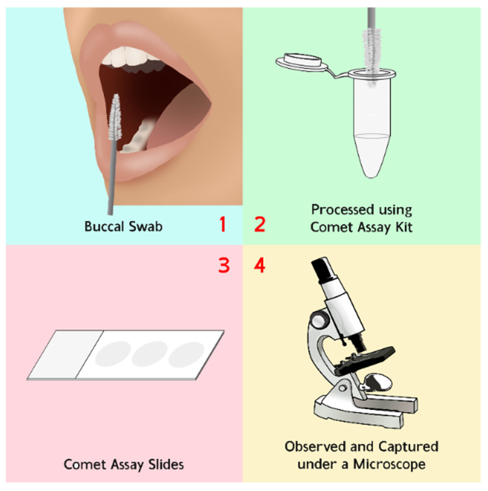
2. Dataset
3. Methods
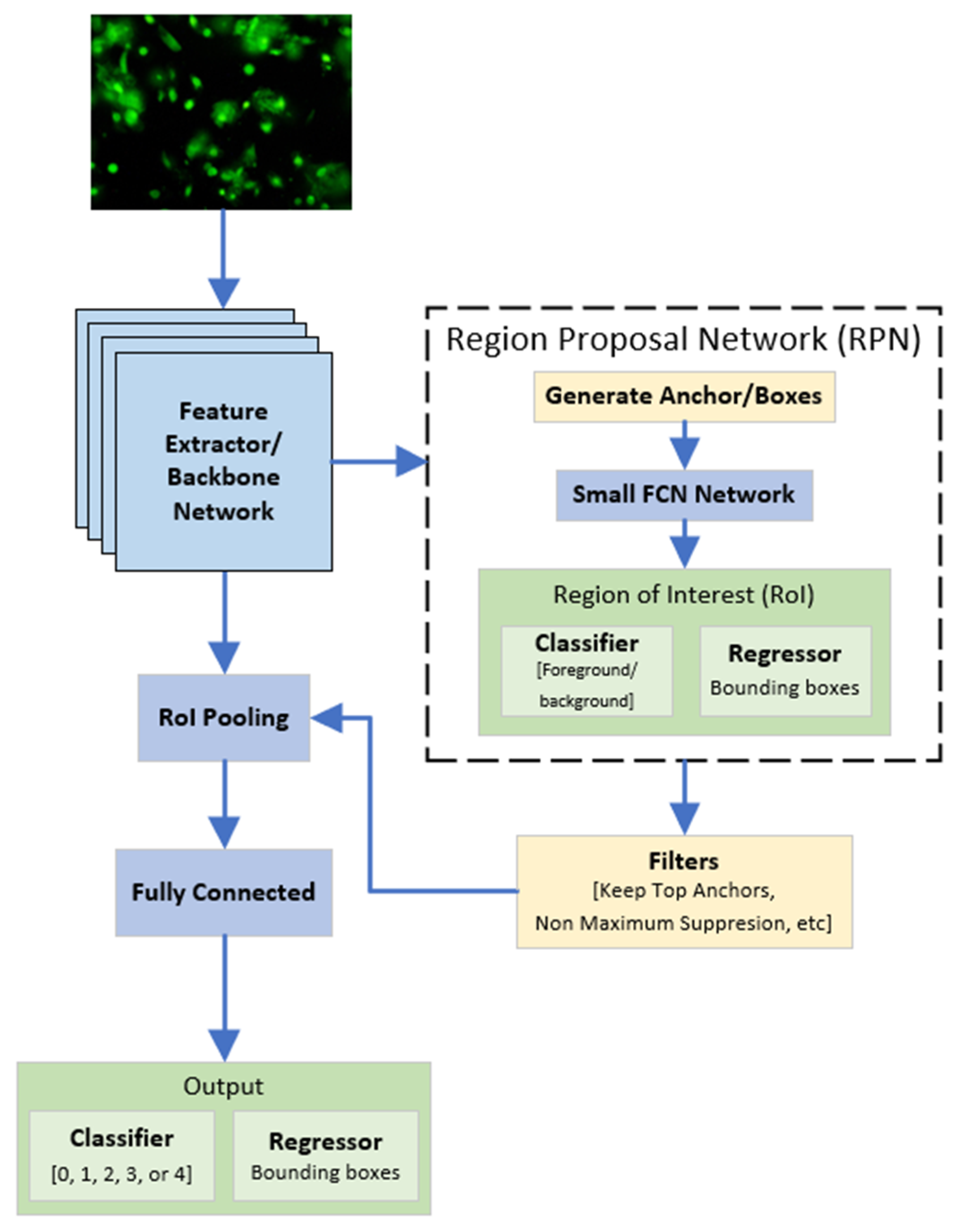
3.1. Faster R-CNN
3.2. Feature Extractor/Backbone Network
3.3. Transfer Learning
3.4. Data Augmentation
3.5. Experiment Scenario
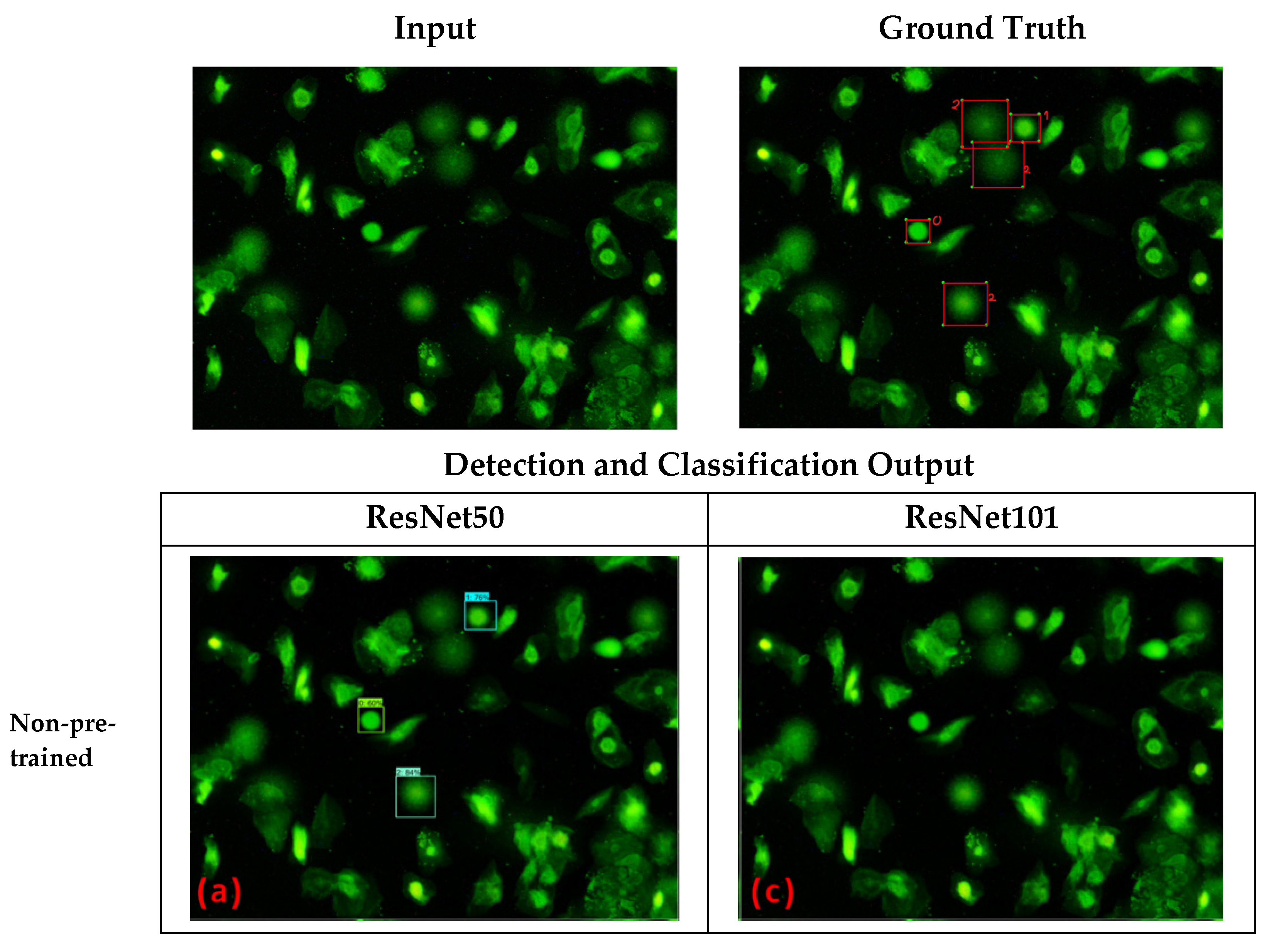
3.5.1. Non-Pre-Trained Model vs. Pre-Trained Model
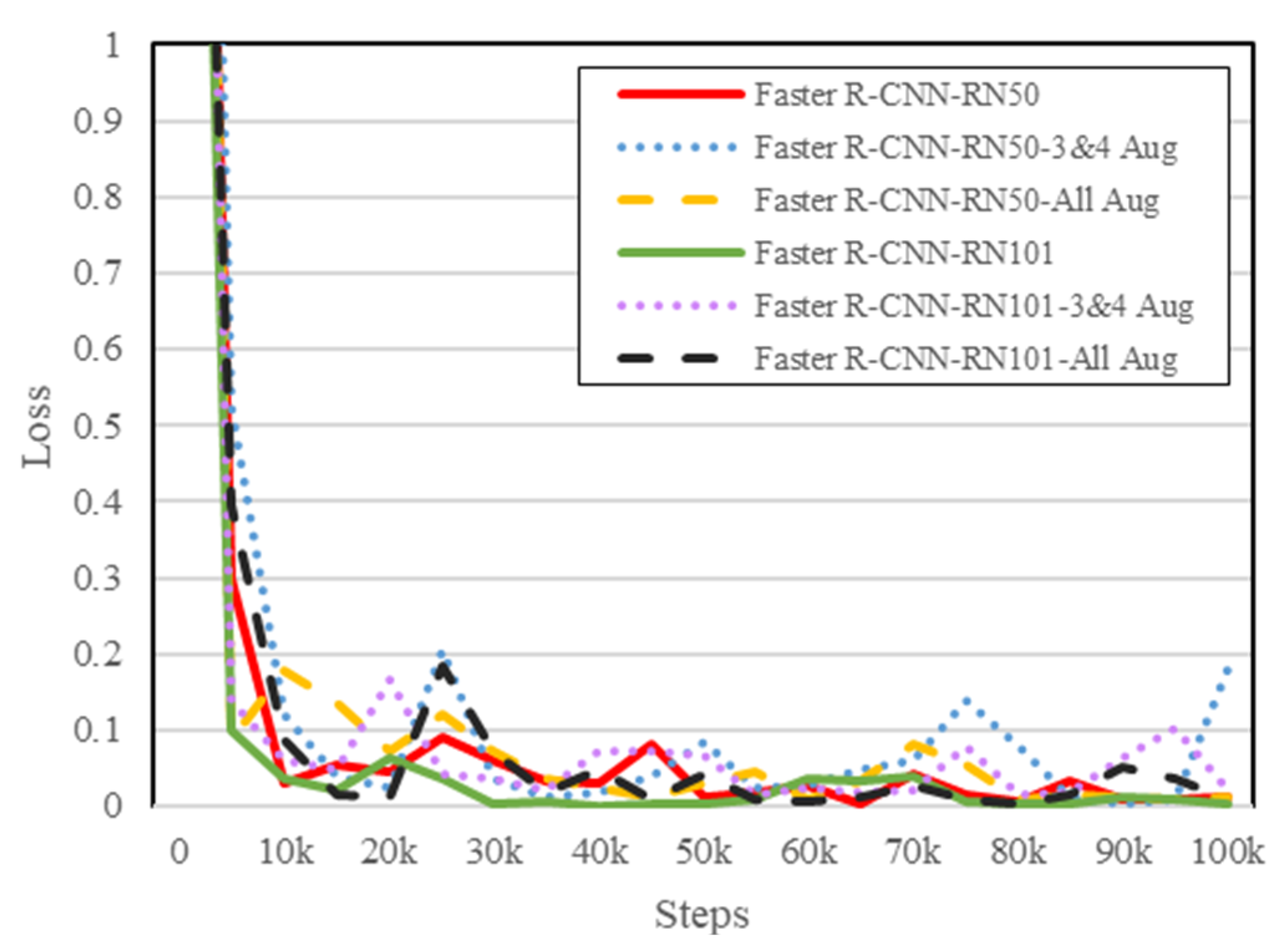
3.5.2. Non-Augmented Dataset vs. Augmented Dataset
3.6. Evaluation Metric
4. Results
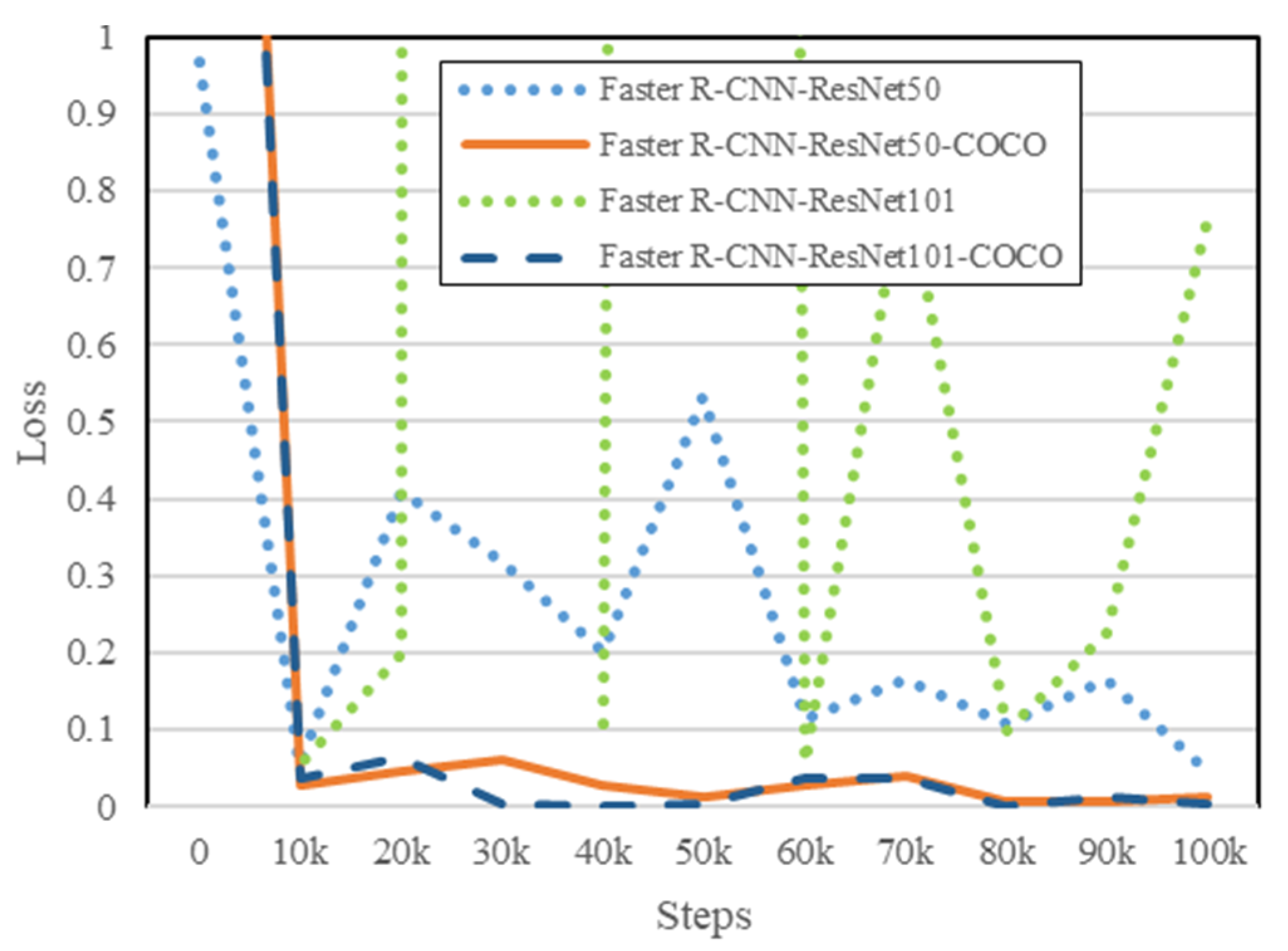
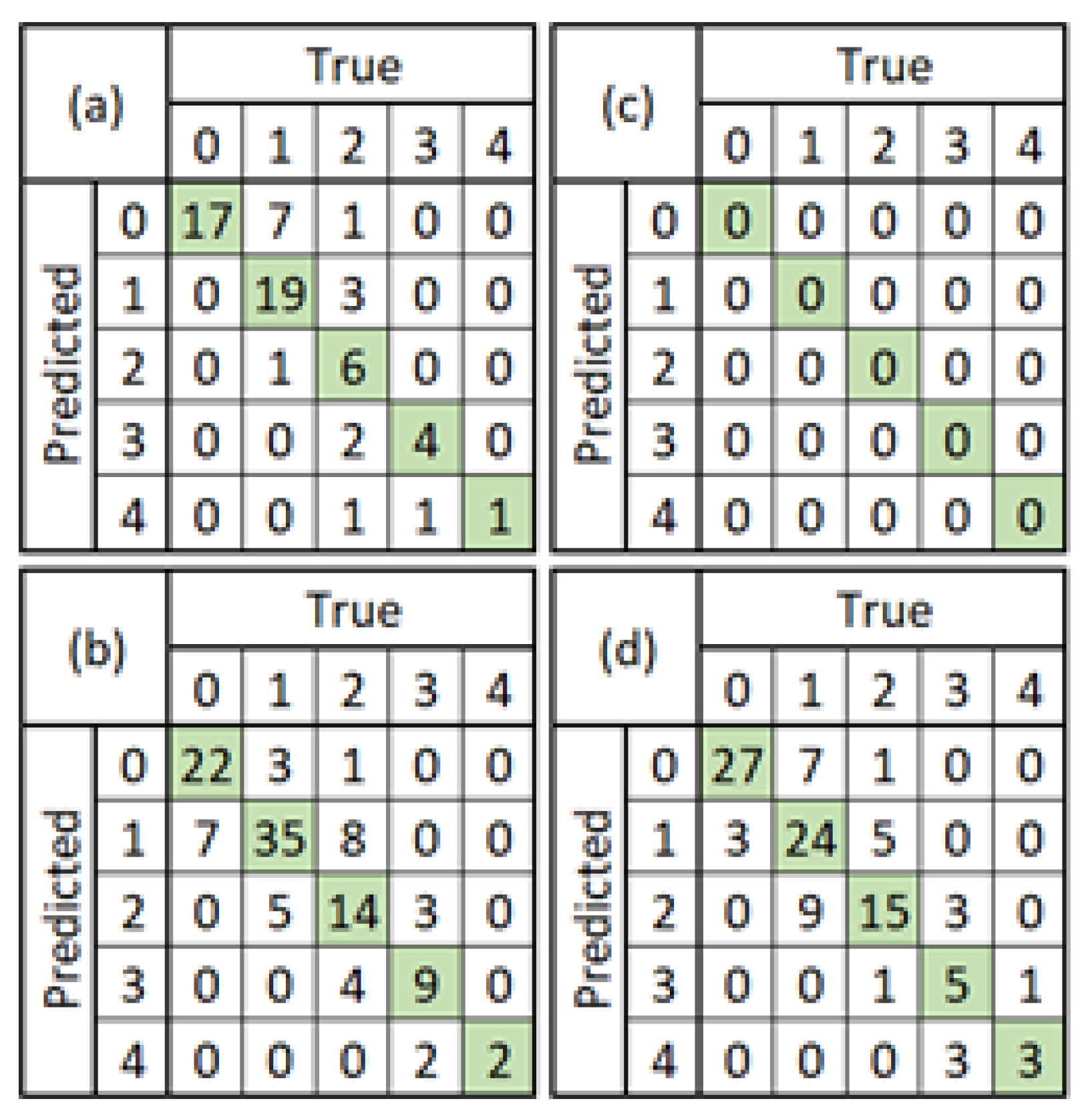
4.1. Non-Pre-Trained vs. Pre-Trained
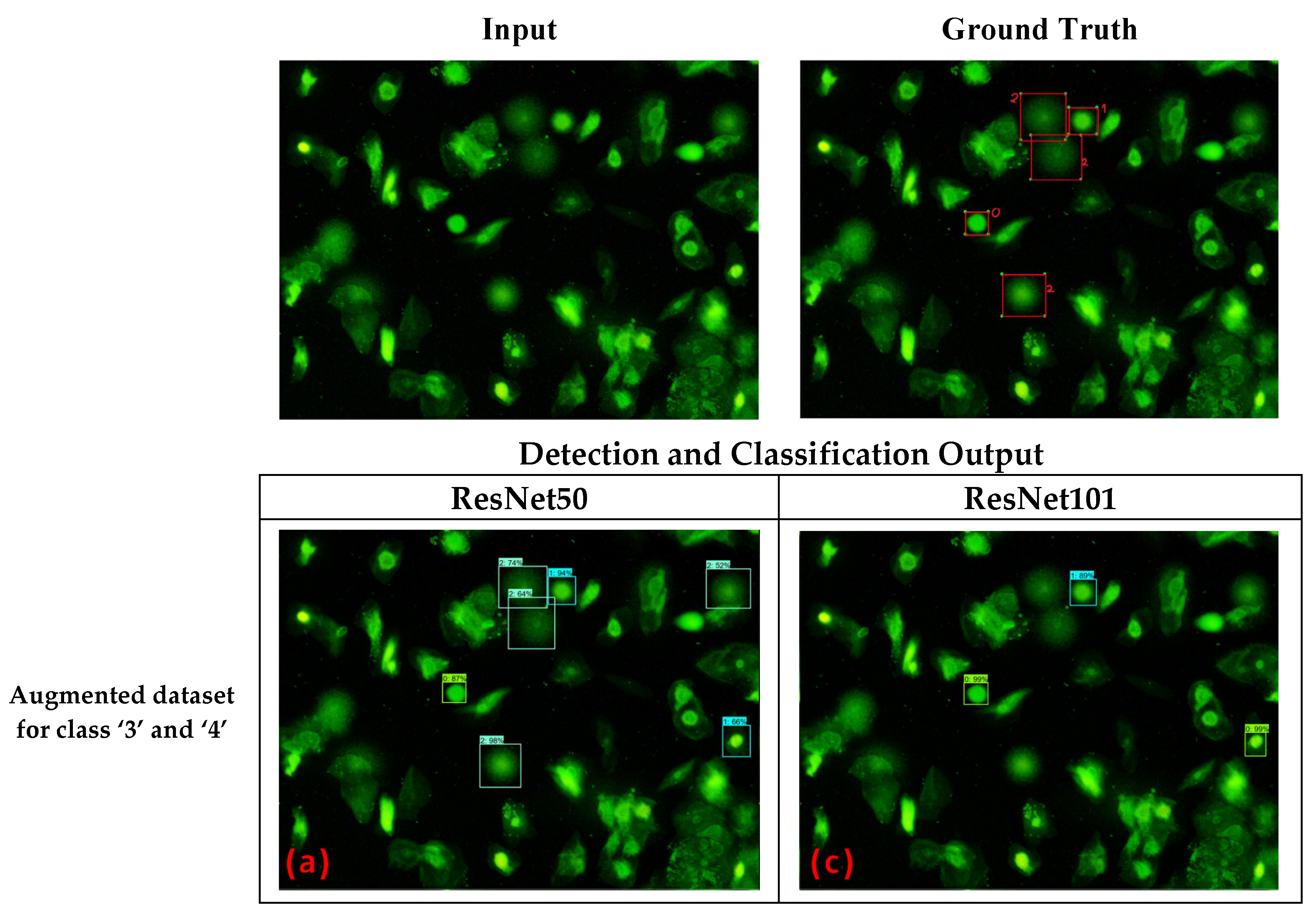
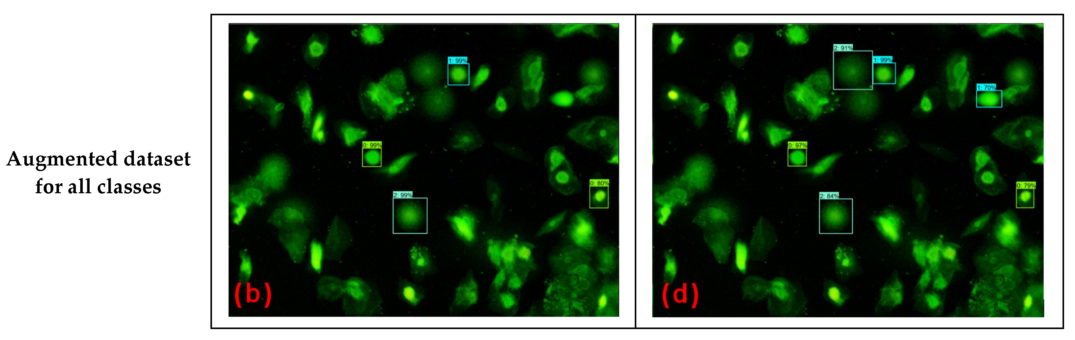
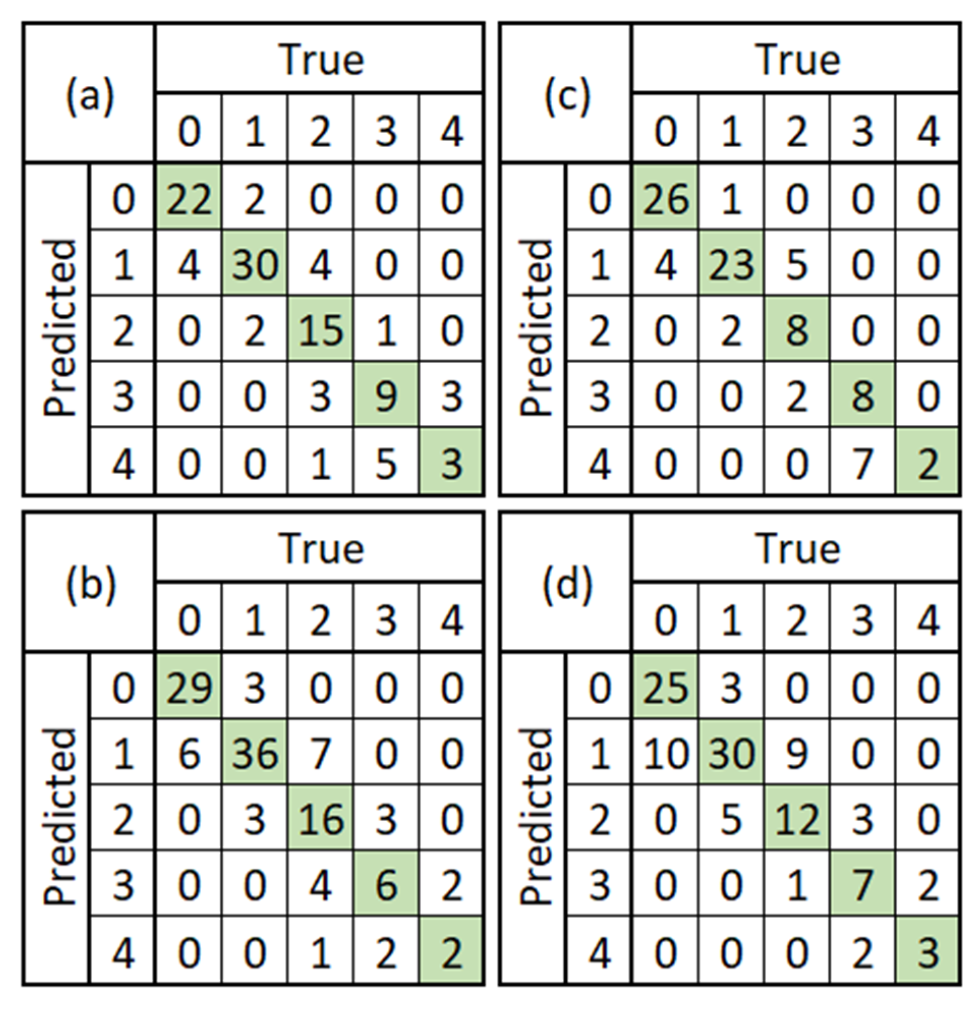
4.2. Non-Augmented Dataset vs. Augmented Dataset
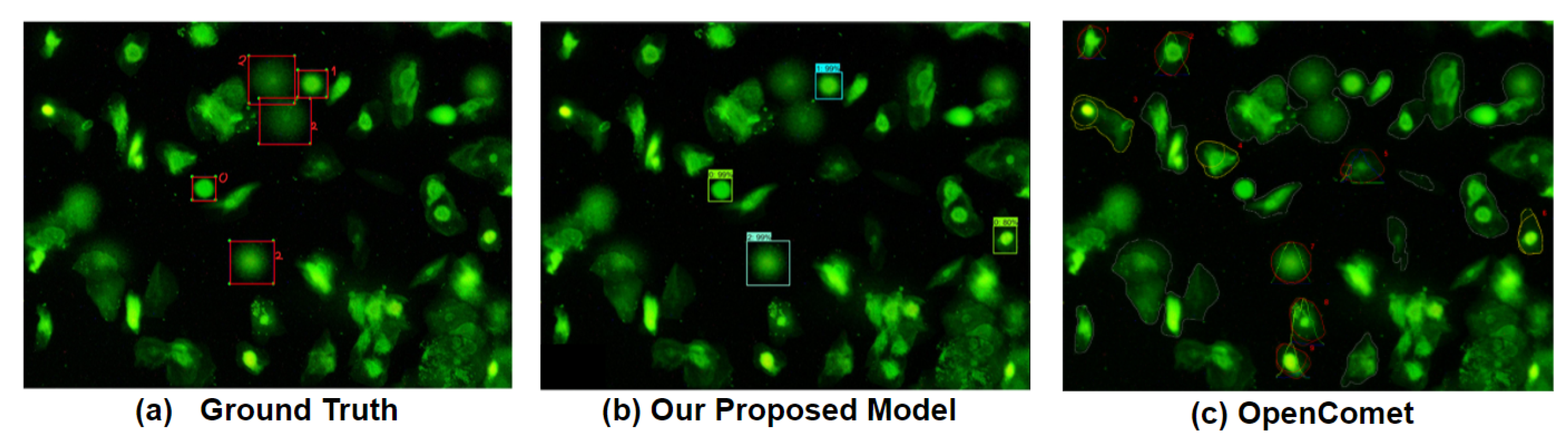
4.3. Faster R-CNN Models vs. OpenComet
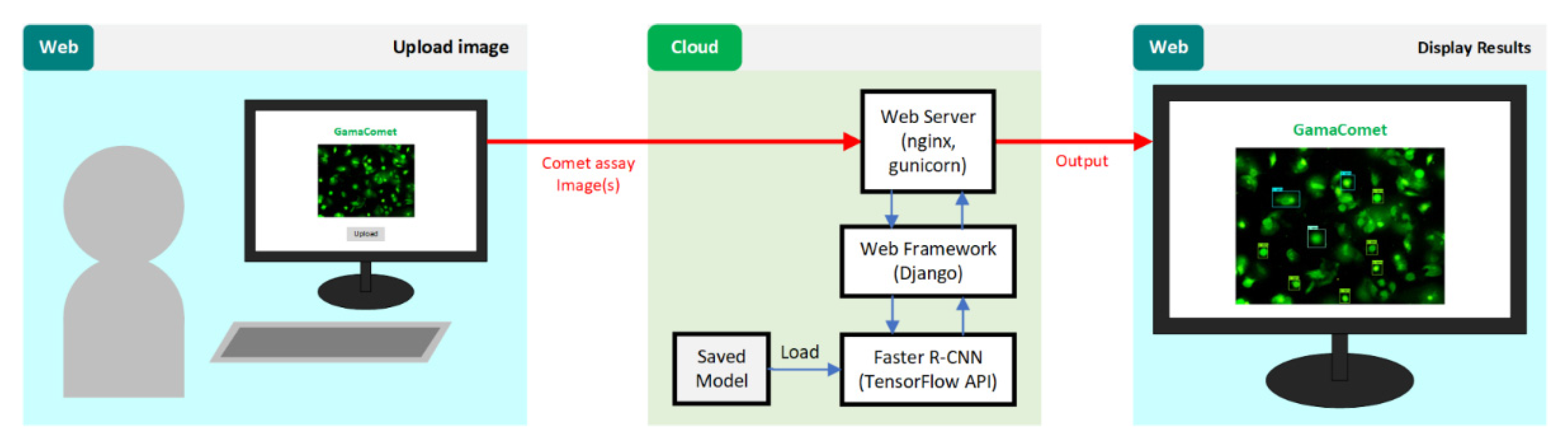
4.4. Implementation of GamaComet
5. Discussion
5.1. Downstream Analysis
5.2. Performance of GamaComet for Another Dataset
6. Conclusions and Future Work
Author Contributions
Funding
Institutional Review Board Statement
Informed Consent Statement
Data Availability Statement
Conflicts of Interest
References
- Olive, P.L.; Banath, J.P. The comet assay: A method to measure DNA damage in individual cells. Nat. Protoc. 2006, 1, 23–29. [Google Scholar] [CrossRef] [PubMed]
- Collins, A.R.; Oscoz, A.A.; Brunborg, G.; Gaivao, I.; Giovannelli, L.; Kruszewski, M.; Smith, C.C.; Štětina, R. The comet assay: Topical issues. Mutagenesis 2008, 23, 143–151. [Google Scholar] [CrossRef] [PubMed]
- Sánchez-Alarcón, J.; Milić, M.; Gómez-Arroyo, S.; Montiel-González, J.M.R.; Valencia-Quintana, R. Assessment of DNA Damage by Comet Assay in Buccal Epithelial Cells: Problems, Achievement, Perspectives. In Environmental Health Risk-Hazardous Factors to Living Species; Larramendy, M.L., Soloneski, S., Eds.; IntechOpen: London, UK, 2016. [Google Scholar]
- Yanuaryska, R.D. Comet Assay Assessment of DNA Damage in Buccal Mucosa Cells Exposed to X-Rays via Panoramic Radiography. J. Dent. Indones. 2018, 25, 53–57. [Google Scholar] [CrossRef]
- Muniz, J.F.; McCauley, L.A.; Pak, V.; Lasarev, M.R.; Kisby, G.E. Effects of sample collec tion and storage conditions on DNA damage in buccal cells from agricultural workers. Mutat. Res. Genet. Toxicol. Environ. Mutagenesis 2011, 720, 8–13. [Google Scholar] [CrossRef] [PubMed]
- Mondal, N.K.; Bhattacharya, P.; Ray, M.R. Assessment of DNA damage by comet assay and fast halo assay in buccal epithelial cells of Indian women chronically exposed to biomass smoke. Int. J. Hyg. Environ. Health 2011, 214, 311–318. [Google Scholar] [CrossRef]
- Końca, K.; Lankoff, A.; Banasik, A.; Lisowska, H.; Kuszewski, T.; Góźdź, S.; Koza, Z.; Wojcik, A. A cross-platform public domain PC image-analysis program for the comet assay. Mutat. Res. Toxicol. Environ. Mutagen. 2002, 534, 15–20. [Google Scholar] [CrossRef]
- Lu, Y.; Liu, Y.; Yang, C. Evaluating In Vitro DNA Damage Using Comet Assay. J. Vis. Exp. 2017, 128, e56450. [Google Scholar] [CrossRef] [PubMed]
- Gyori, B.M.; Venkatachalam, G.; Thiagarajan, P.S.; Hsu, D.; Clement, M. OpenComet: An automated tool for comet assay image analysis. Redox Biol. 2014, 12, 457–465. [Google Scholar] [CrossRef]
- Ganapathy, S.; Muraleedharan, A.; Sathidevi, P.S.; Chand, P.; Rajkumar, R.P. CometQ: An automated tool for the detection and quantification of DNA damage using comet assay image analysis. Comput. Methods Programs Biomed. 2016, 133, 143–154. [Google Scholar] [CrossRef] [PubMed]
- Hong, Y.; Han, H.-J.; Lee, H.; Lee, D.; Ko, J.; Hong, Z.-Y.; Lee, J.-Y.; Seok, J.-H.; Lim, H.S.; Son, W.-C.; et al. Deep learning method for comet segmentation and comet assay image analysis. Sci. Rep. 2020, 10, 1–12. [Google Scholar] [CrossRef]
- Afiahayati Anarossi, E.; Yanuaryska, R.D.; Nuha, F.U.; Mulyana, S. Comet Assay Classification for Buccal Mucosa’s DNA Damage Measurement with Super Tiny Dataset Using Transfer Learning. Intell. Inf. Database Syst. Recent Dev. 2020, 830, 279. [Google Scholar]
- Hafiyan, Y.T.; Afiahayati Yanuaryska, R.D.; Anarossi, E.; Sutanto, V.M.; Triyanto, J.; Sakakibara, Y. A Hybrid Convolutional Neural Network-Extreme Learning Machine with Augmented Dataset for DNA Damage Classification using Comet Assay from Buccal Mucosa Sample. Int. J. Innov. Comput. Inf. Control 2021, 17, 1191–11201. [Google Scholar]
- Rosati, R.; Romeo, L.; Silvestri, S.; Marcheggiani, F.; Tiano, L.; Frontoni, E. Faster R-CNN approach for detection and quantification of DNA damage in comet assay images. Comput. Biol. Med. 2020, 123, 103912. [Google Scholar] [CrossRef] [PubMed]
- Ren, S.; He, K.; Girshick, R.; Sun, J. Faster R-CNN: Towards Real-Time Object Detection with Region Proposal Networks. IEEE Trans. Pattern Anal. Mach. Intell. 2016, 39, 1137–1149. [Google Scholar] [CrossRef] [PubMed]
- Koziarski, M.; Cyganek, B. Impact of Low Resolution on Image Recognition with Deep Neural Networks: An Experimental Study. Int. J. Appl. Math. Comput. Sci. 2018, 28, 735–744. [Google Scholar] [CrossRef]
- Yosinski, J.; Clune, J.; Bengio, Y.; Lipson, H. How transferable are features in deep neural networks? In Proceedings of the 27th International Conference on Neural Information Processing Systems (NIPS), Montreal, QC, Canada, 8–13 December 2014; pp. 3320–3328. [Google Scholar]
- Shorten, C.; Khoshgoftaar, T.M. A survey on Image Data Augmentation for Deep Learning. J. Big Data 2019, 6, 60. [Google Scholar] [CrossRef]
- Girshick, R.; Donahue, J.; Darrell, T.; Malik, J. Rich feature hierarchies for accurate object detection and semantic segmen-tation. In Proceedings of the 2014 IEEE Conference on Computer Vision and Pattern Recognition (CVPR), Columbus, OH, USA, 23–28 June 2014; pp. 580–587. [Google Scholar]
- Girshick, R. Fast r-cnn. In Proceedings of the 2015 IEEE International Conference on Computer Vision (ICCV), Santiago, Chile, 7–13 December 2015; pp. 1440–1448. [Google Scholar]
- Huang, J.; Rathod, V.; Sun, C.; Zhu, M.; Korattikara, A.; Fathi, A.; Fischer, I.; Wojna, Z.; Song, Y.; Guadarrama, S.; et al. Speed/accuracy trade-offs for modern convolutional object detectors. In Proceedings of the 2017 IEEE Conference on Computer Vision and Pattern Recognition Workshops (CVPRW), Honolulu, HI, USA, 21–26 July 2017; pp. 7310–7311. [Google Scholar]
- He, K.; Zhang, X.; Ren, S.; Sun, J. Deep residual learning for image recognition. In Proceedings of the 2016 IEEE Conference on Computer Vision and Pattern Recognition Workshops (CVPRW), Las Vegas, NV, USA, 26 June–1 July 2016; pp. 770–778. [Google Scholar]
- Lin, T.Y.; Maire, M.; Belongie, S.; Hays, J.; Perona, P.; Ramanan, D.; Dollar, P.; Zitnick, C.L. Microsoft COCO: Common Objects in Context. In Proceedings of the 2014 European Conference on Computer Vision, Zurich, Switzerland, 6–12 September 2014; pp. 740–755. [Google Scholar]


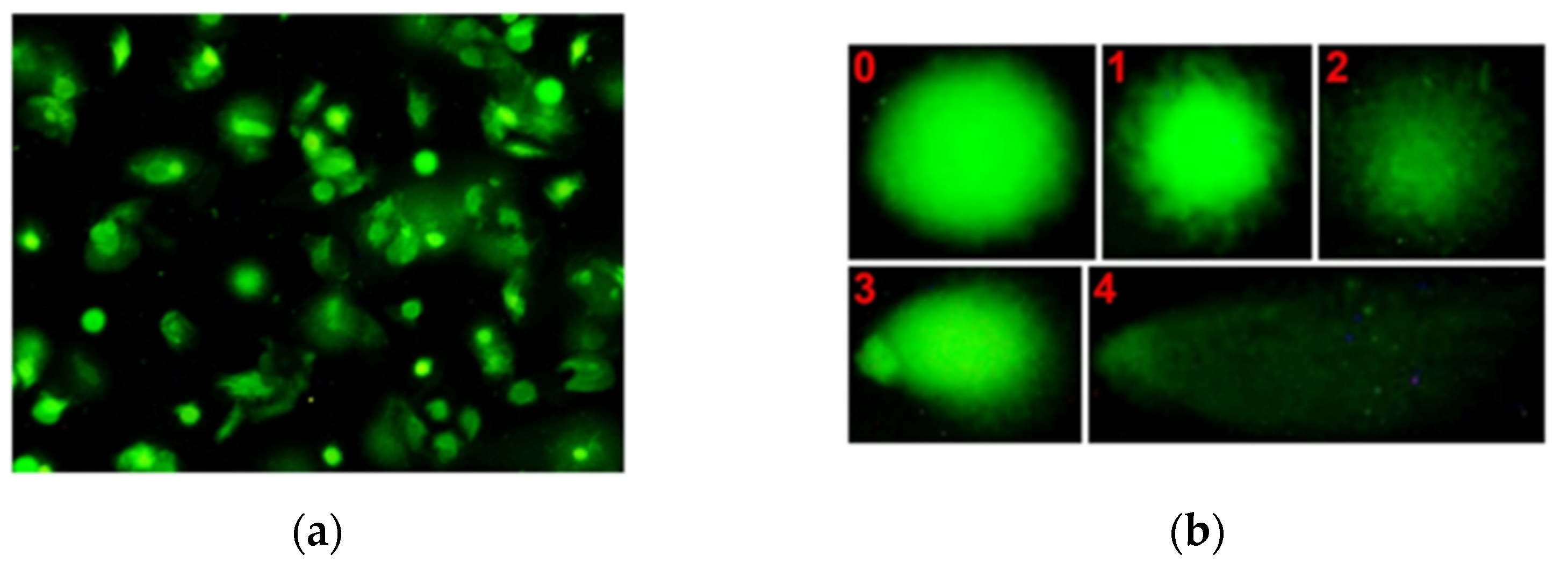
| Class | Full Set (275 Images) | Training Set (193 Images) | Validation Set (82 Images) |
|---|---|---|---|
| 0 | 127 comets | 88 comets | 39 comets |
| 1 | 197 comets | 143 comets | 54 comets |
| 2 | 128 comets | 90 comets | 38 comets |
| 3 | 48 comets | 31 comets | 17 comets |
| 4 | 19 comets | 13 comets | 6 comets |
| Total | 519 comets | 365 comets | 154 comets |
| Class | Training Set | Validation Set (82 Images) | |
|---|---|---|---|
| Before Augmentation (193 Images) | After Augmentation (277 Images) | ||
| 0 | 88 comets | 88 comets | 39 comets |
| 1 | 143 comets | 143 comets | 54 comets |
| 2 | 90 comets | 90 comets | 38 comets |
| 3 | 31 comets | 217 comets | 17 comets |
| 4 | 13 comets | 91 comets | 6 comets |
| Total | 365 comets | 629 comets | 154 comets |
| Class | Training Set | Validation Set (82 Images) | |
|---|---|---|---|
| Before Augmentation (193 Images) | After Augmentation (579 Images) | ||
| 0 | 88 comets | 264 comets | 39 comets |
| 1 | 143 comets | 429 comets | 54 comets |
| 2 | 90 comets | 270 comets | 38 comets |
| 3 | 31 comets | 93 comets | 17 comets |
| 4 | 13 comets | 39 comets | 6 comets |
| Total | 365 comets | 1095 comets | 154 comets |
| Detection | Classification | |||
|---|---|---|---|---|
| Accuracy | F1-Score | Accuracy | F1-Score | |
| Faster R-CNN-ResNet50 | 93.66% | 62.24% | 41.56% | 60.18% |
| Faster R-CNN-ResNet50-COCO | 95.49% | 76.54% | 62.99% | 57.42% |
| Faster R-CNN-ResNet101 | N/A | N/A | N/A | N/A |
| Faster R-CNN-ResNet101-COCO | 94.51% | 70.34% | 52.60% | 54.47% |
| Detection | Classification | |||
|---|---|---|---|---|
| Accuracy | F1-Score | Accuracy | F1-Score | |
| Faster R-CNN-ResNet50-COCO | 95.49% | 76.54% | 62.99% | 57.42% |
| Faster R-CNN-ResNet50-COCO-3&4 Aug. | 95.00% | 72.31% | 55.19% | 55.78% |
| Faster R-CNN-ResNet50-COCO-All Aug. | 95.85% | 78.50% | 63.64% | 58.03% |
| Faster R-CNN-ResNet101-COCO | 94.51% | 70.34% | 52.60% | 54.47% |
| Faster R-CNN-ResNet101-COCO-3&4 Aug. | 94.45% | 71.64% | 62.34% | 59.42% |
| Faster R-CNN-ResNet101-COCO-All Aug. | 95.37% | 75.23% | 59.74% | 57.95% |
| Accuracy | F1-Score | |
|---|---|---|
| Faster R-CNN-ResNet50 | 93.66% | 62.24% |
| Faster R-CNN-ResNet50-COCO | 95.49% | 76.54% |
| Faster R-CNN-ResNet50-COCO-3&4 Aug. | 95.00% | 72.31% |
| Faster R-CNN-ResNet50-COCO-All Aug. | 95.85% | 78.50% |
| Faster R-CNN-ResNet101 | N/A | N/A |
| Faster R-CNN-ResNet101-COCO | 94.51% | 70.34% |
| Faster R-CNN-ResNet101-COCO-3&4 Aug. | 94.45% | 71.64% |
| Faster R-CNN-ResNet101-COCO-All Aug. | 95.37% | 75.23% |
| OpenComet [9] | 76.52% | 29.87% |
| PatientNo | Sample ID | Collection Date | Sex | Age (Years) | Smoking Habit |
|---|---|---|---|---|---|
| 1 | 07092018_1 | 7 September 2018 | Female | 24 | No |
| 2 | 07092018_2 | 7 September 2018 | Female | 22 | No |
| 3 | 07092018_3 | 7 September 2018 | Female | 22 | No |
| 4 | 07092018_4 | 7 September 2018 | Female | 27 | No |
| 5 | 07092018_5 | 7 September 2018 | Female | 21 | No |
| 6 | 07092018_6 | 7 September 2018 | Male | 22 | No |
| 7 | 07092018_7 | 7 September 2018 | Female | 22 | No |
| 8 | 13092018_1 | 13 September 2018 | Female | 23 | No |
| 9 | 13092018_2 | 13 September 2018 | Female | 22 | No |
| 10 | 13092018_3 | 13 September 2018 | Female | 21 | No |
| 11 | 13092018_4 | 13 September 2018 | Female | 22 | No |
| 12 | 13092018_5 | 13 September 2018 | Female | 22 | No |
| 13 | 13092018_6 | 13 September 2018 | Female | 22 | No |
| 14 | 13092018_7 | 13 September 2018 | Female | 24 | No |
| 15 | 13092018_8 | 13 September 2018 | Female | 25 | No |
| 16 | 14092018_1 | 14 September 2018 | Male | 18 | No |
| 17 | 14092018_2 | 14 September 2018 | Female | 25 | No |
| 18 | 14092018_3 | 14 September 2018 | Female | 23 | No |
| 19 | 14092018_4 | 14 September 2018 | Male | 23 | Yes |
| 20 | 14092018_5 | 14 September 2018 | Male | 24 | Yes |
| 21 | 14092018_6 | 14 September 2018 | Male | 25 | Yes |
| 22 | 14092018_7 | 14 September 2018 | Male | 24 | Yes |
| 23 | 14092018_8 | 14 September 2018 | Male | 20 | Yes |
| 24 | 14092018_9 | 14 September 2018 | Male | 23 | Yes |
| Class | Testing Dataset (43 Images) |
|---|---|
| 0 | 12 comets |
| 1 | 15 comets |
| 2 | 11 comets |
| 3 | 25 comets |
| 4 | 10 comets |
| Total | 73 comets |
| Accuracy | ||
|---|---|---|
| Detection | Classification | |
| GamaComet | 81.34% | 66.67% |
| OpenComet [9] | 11.5% | - |
Publisher’s Note: MDPI stays neutral with regard to jurisdictional claims in published maps and institutional affiliations. |
© 2022 by the authors. Licensee MDPI, Basel, Switzerland. This article is an open access article distributed under the terms and conditions of the Creative Commons Attribution (CC BY) license (https://creativecommons.org/licenses/by/4.0/).
Share and Cite
Afiahayati; Anarossi, E.; Yanuaryska, R.D.; Mulyana, S. GamaComet: A Deep Learning-Based Tool for the Detection and Classification of DNA Damage from Buccal Mucosa Comet Assay Images. Diagnostics 2022, 12, 2002. https://doi.org/10.3390/diagnostics12082002
Afiahayati, Anarossi E, Yanuaryska RD, Mulyana S. GamaComet: A Deep Learning-Based Tool for the Detection and Classification of DNA Damage from Buccal Mucosa Comet Assay Images. Diagnostics. 2022; 12(8):2002. https://doi.org/10.3390/diagnostics12082002
Chicago/Turabian StyleAfiahayati, Edgar Anarossi, Ryna Dwi Yanuaryska, and Sri Mulyana. 2022. "GamaComet: A Deep Learning-Based Tool for the Detection and Classification of DNA Damage from Buccal Mucosa Comet Assay Images" Diagnostics 12, no. 8: 2002. https://doi.org/10.3390/diagnostics12082002