Author Contributions
Conceptualization, S.N.; Funding acquisition, J.G.E. and L.G.S.; Investigation, S.N.; Methodology, S.N. and B.L.; Resources, M.M., S.K., C.J.M., O.H.C. and J.G.E.; Software, S.N. and W.W.; Supervision, J.G.E. and L.G.S.; Validation, S.N.; Writing—original draft, S.N.; Writing—review & editing, L.G.S. All authors have read and agreed to the published version of the manuscript.
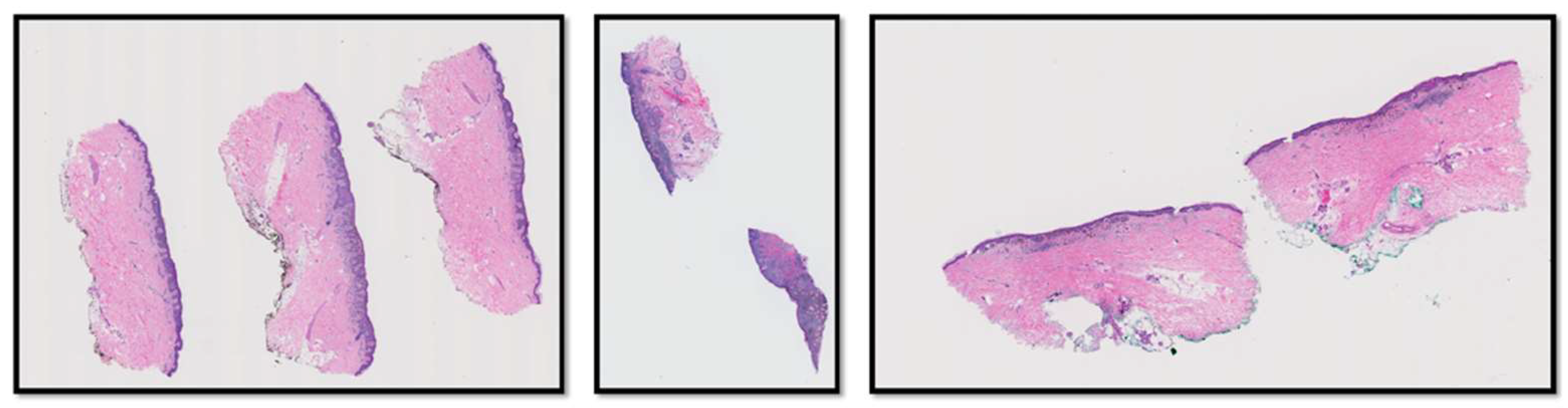
Figure 1.
Three examples of WSIs in the M-Path dataset. The left image is a case with class IV diagnosis (invasive melanoma stage T1a), the middle image is a case with class V diagnosis (invasive melanoma stage ≥ T1b), and the right image is a case with class IV diagnosis (invasive melanoma stage T1a).
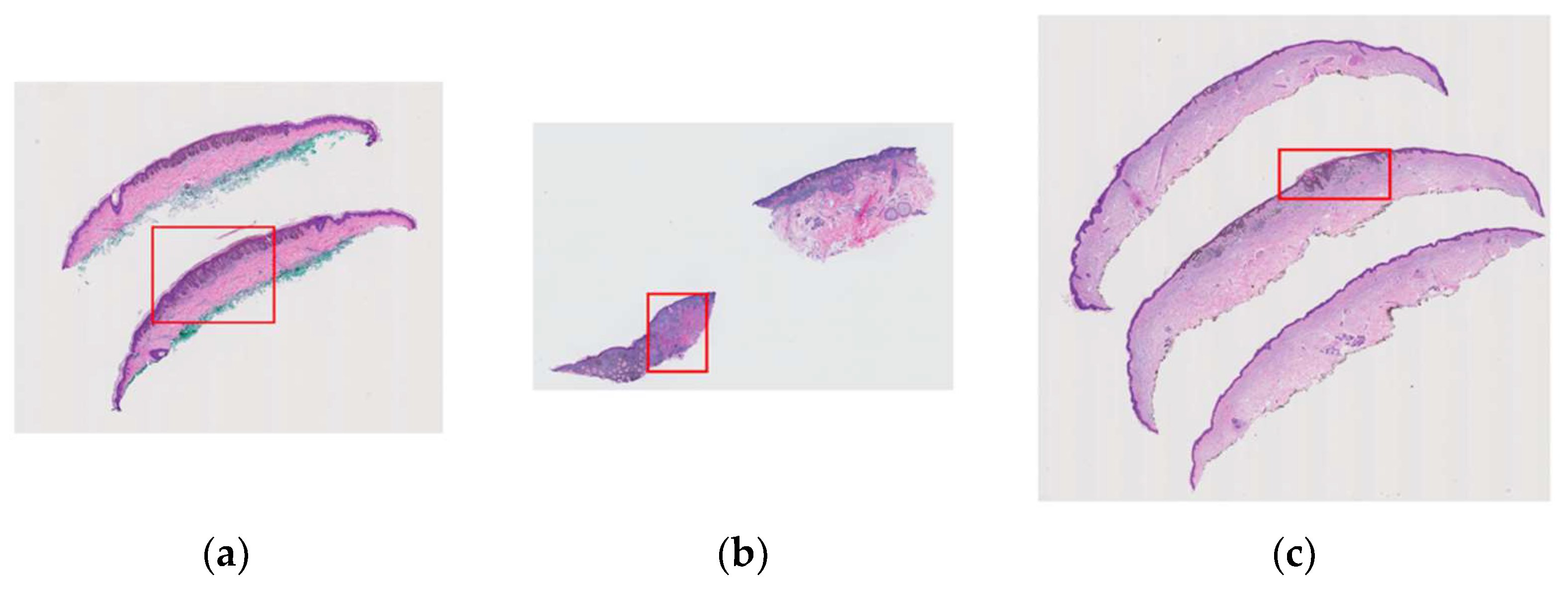
Figure 2.
Examples of variable-sized region of interests (ROI) assigned by pathologists that contain important diagnostic information are shown in red boxes: (a) a case with class II diagnosis (moderately dysplastic nevus), (b) a case with class V diagnosis (invasive melanoma stage ≥ T1b), (c) a case with class IV diagnosis (invasive melanoma stage T1a).
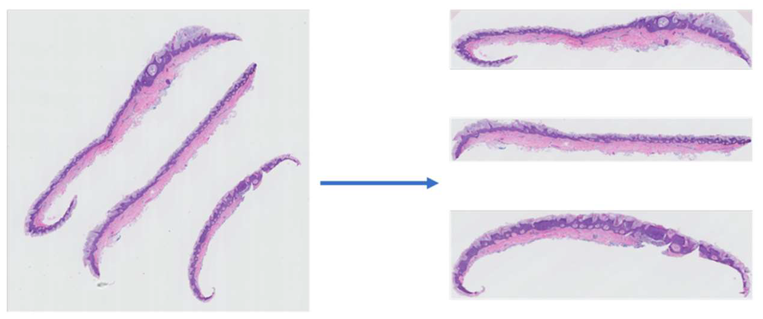
Figure 3.
An example of a WSI (left) and its corresponding slice extraction (right).
Figure 3.
An example of a WSI (left) and its corresponding slice extraction (right).
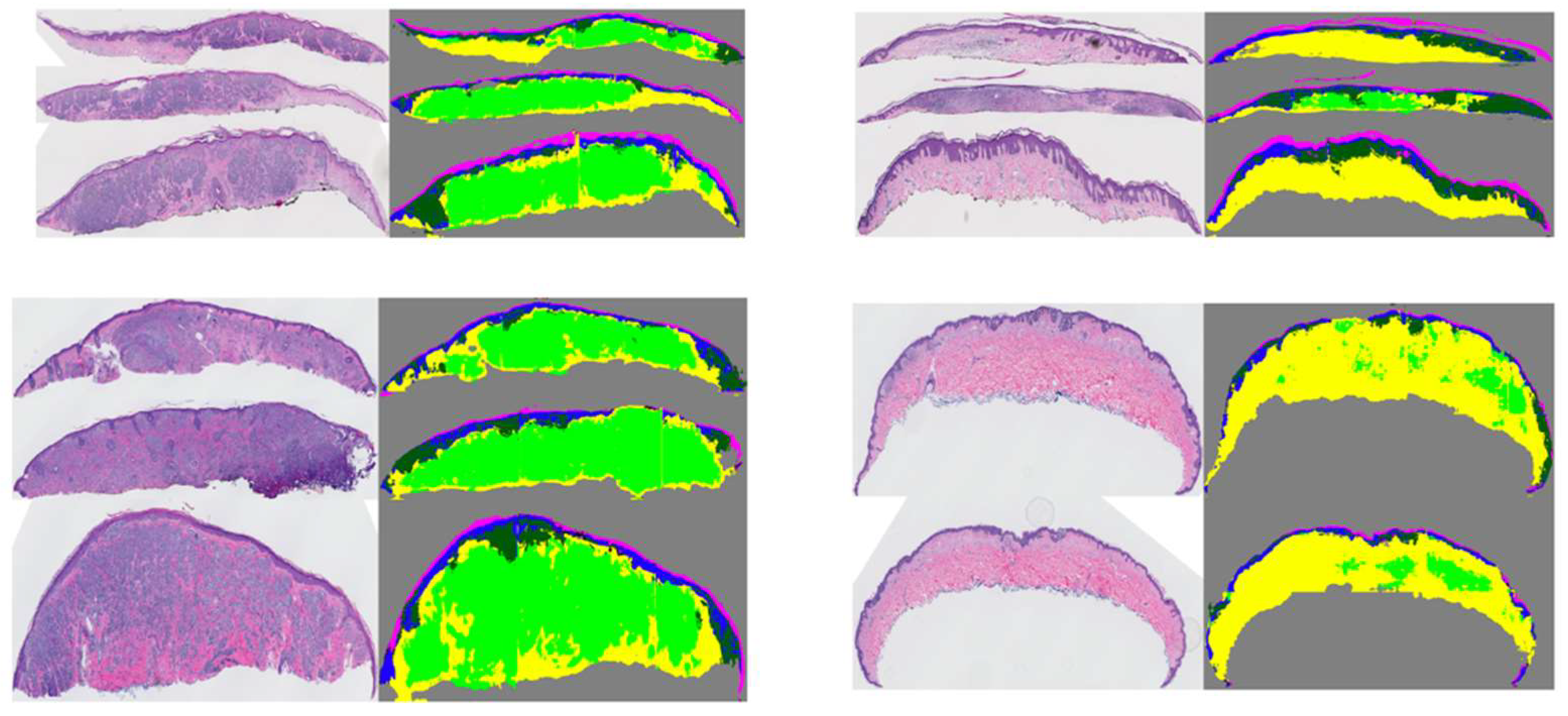
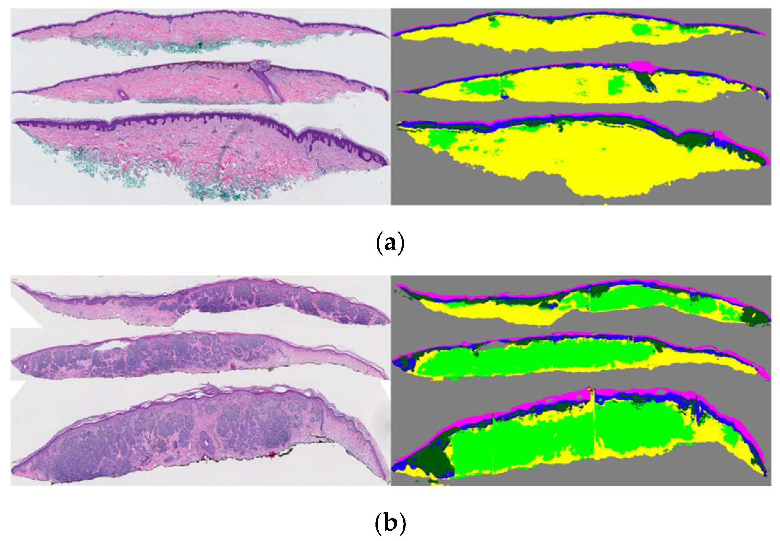
Figure 4.
Examples of original WSIs and their corresponding segmentation mask. The segmentation images contain the dermis, epidermis, stratum corneum, background, dermal, and epidermal nests. The model was trained on coarse and sparse annotations.
Figure 4.
Examples of original WSIs and their corresponding segmentation mask. The segmentation images contain the dermis, epidermis, stratum corneum, background, dermal, and epidermal nests. The model was trained on coarse and sparse annotations.
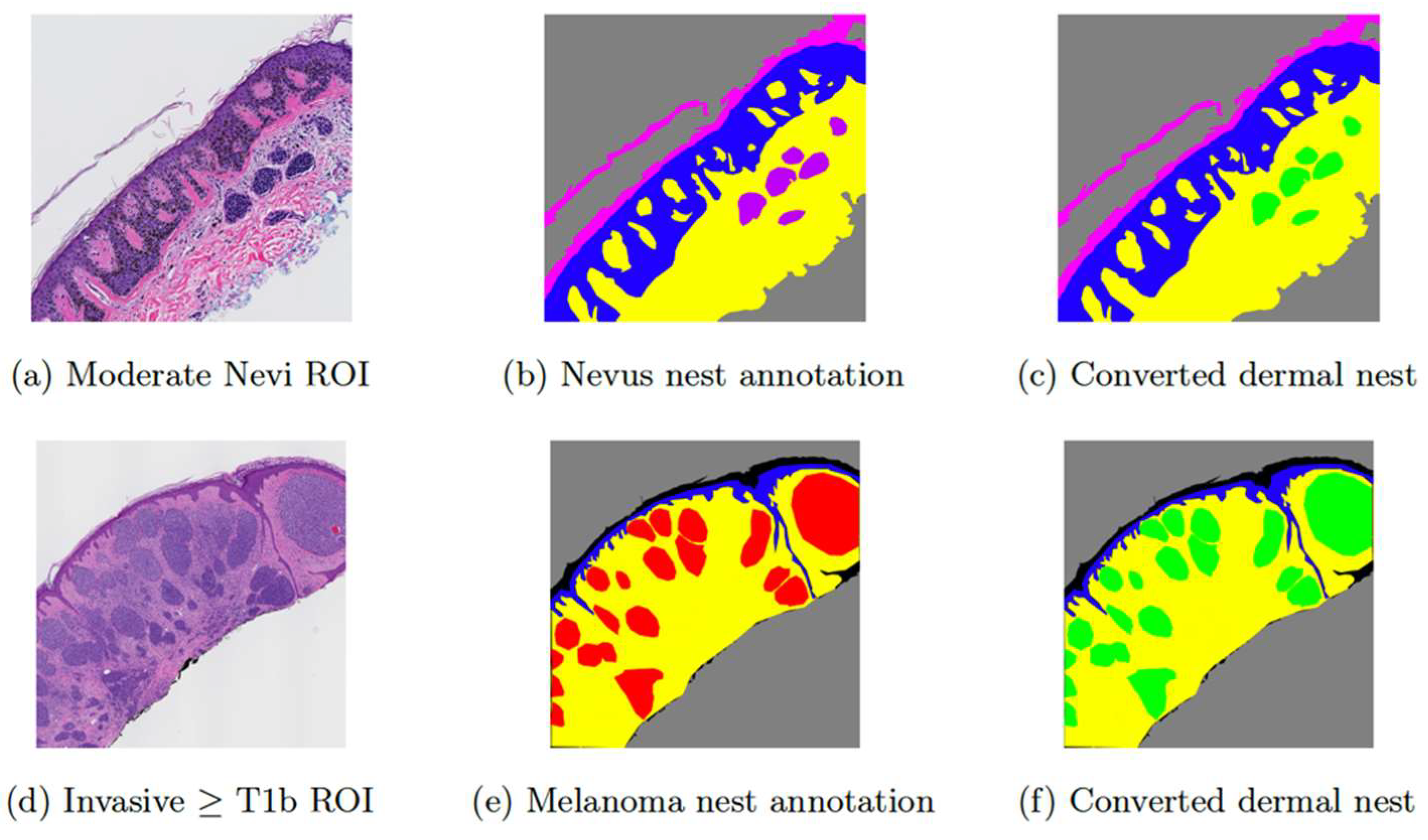
Figure 5.
Examples of input ROI images and their corresponding annotations. (a) shows a moderate Nevi ROI image, (b) shows the original Nevus dermal nest annotation in purple, (c) is the converted version of (b) in which purple annotations of nevus dermal nests (DMN-N) are converted to green markings of dermal nest (DMN), (d) shows an invasive melanoma stage ≥ T1b ROI image, (e) shows the original melanoma nests annotation in red, (f) is the converted version of (e) in which red annotation of melanoma dermal nests (DMN-M) are converted to green markings of dermal nest (DMN).
Figure 6.
Example of dermal nest segmentation (in light green) on WSI: (a) a moderate nevi case; all the dermal nests are nevi type. (b) An invasive melanoma stage ≥ T1b case; the segmented dermal nests might contain both nevi and melanoma dermal nests.
Figure 6.
Example of dermal nest segmentation (in light green) on WSI: (a) a moderate nevi case; all the dermal nests are nevi type. (b) An invasive melanoma stage ≥ T1b case; the segmented dermal nests might contain both nevi and melanoma dermal nests.
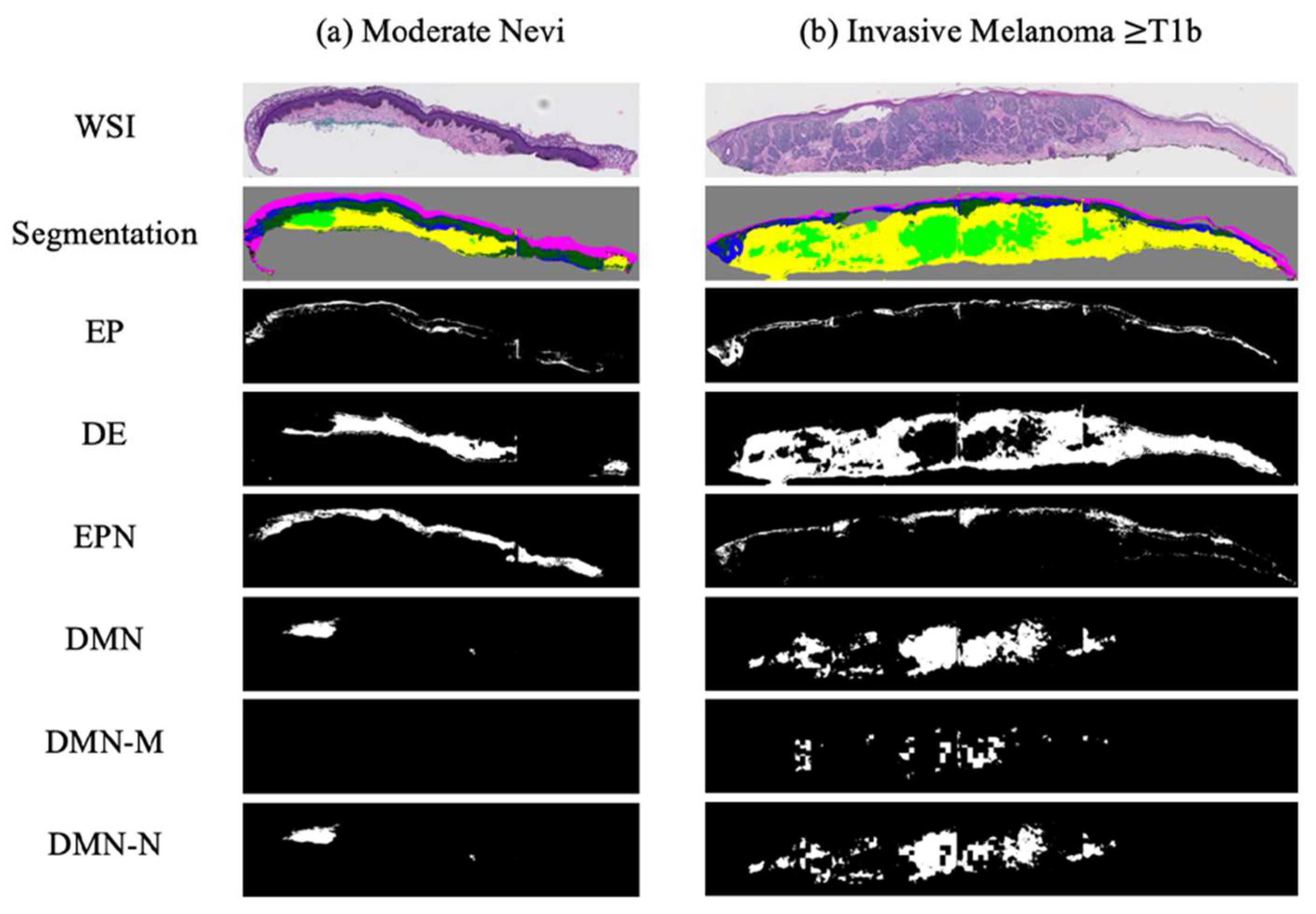
Figure 7.
Examples of binarized segmentation masks: (a) a moderate nevi case; (b) an invasive melanoma stage ≥ T1b. From top to bottom, one extracted slice from a WSI, all segmentation masks in one mask (containing EP, DE, EPN, and DMN), binary Epidermis (EP) mask, binary dermis (DE) mask, binary epidermal nest (EPN) mask, binary dermal nest (DMN) mask, binary melanoma dermal nest (DMN-M), and binary nevus dermal nest (DMN-N) mask are shown.
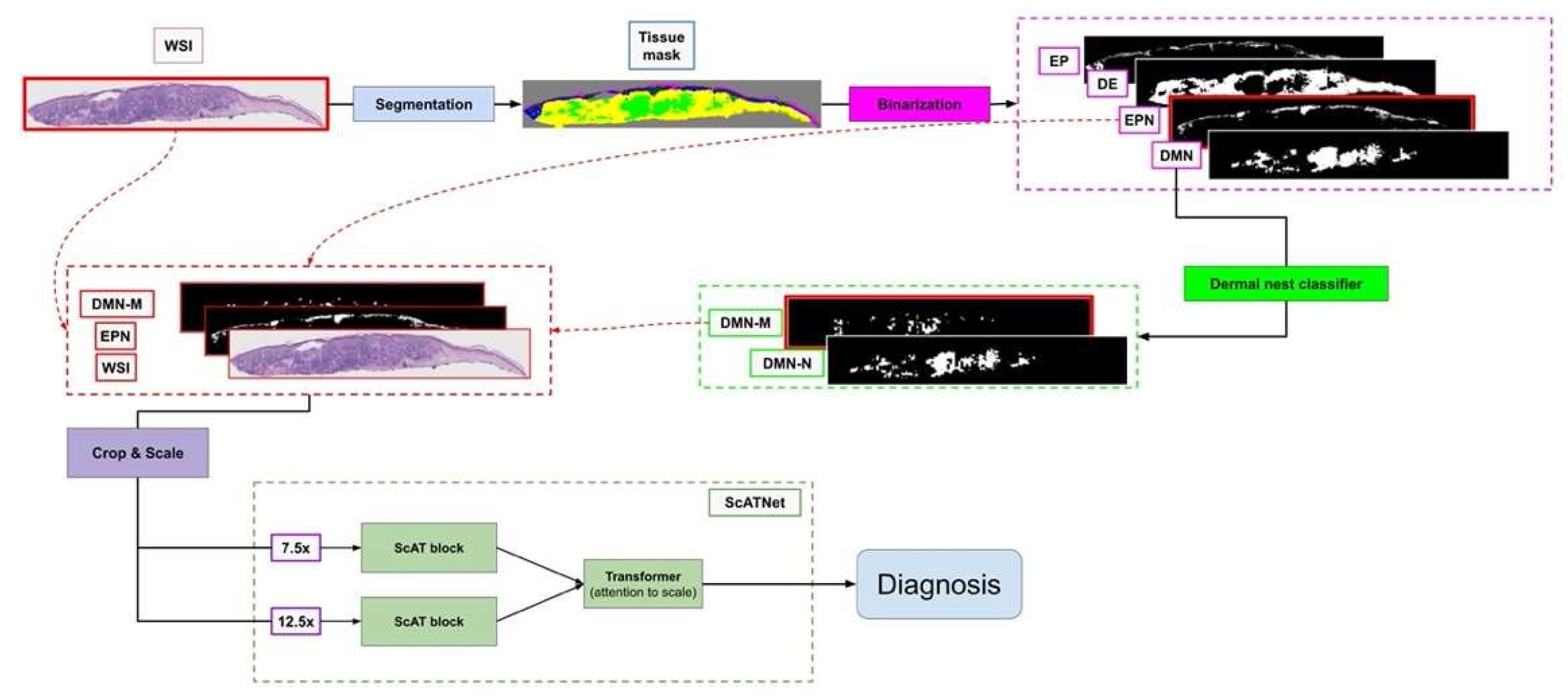
Figure 8.
Overview of our diagnosis pipeline. The WSI goes to the segmentation pipeline to generate a tissue segmentation mask. Then, four clinically important tissue structures: epidermis (EP), dermis (DE), epidermal nest (EPN), and dermal nest (DMN) will be extracted into four corresponding binary masks. Extracted Dermal Nests will go through a dermal nests classification step to generate two sub-categories of melanoma dermal nest (DMN-M) and nevus dermal nest (DMN-N). Then, the selected tissue masks based on the experiment will be concatenated to the RGB channels of the WSI image. Each image will be cropped into smaller patches afterward. The patches go through the ScATNet pipeline that extracts patch embeddings, then, using contextualized patch-embedding and scale-aware embedding across available scales, chooses the diagnostic class of the case from mild and moderate dysplastic nevi (MMD), melanoma in situ and severely dysplastic nevi (MIS), invasive melanoma T1a (T1a) and melanoma invasive ≥ T1b (T1b). Note that the concatenated masks to the WSI (DMN-M and EPN) and ScATNet scales (7.5× and 12.5×) shown in this figure are just one example of our multiple experimental studies.
![Diagnostics 12 01713 g008]()
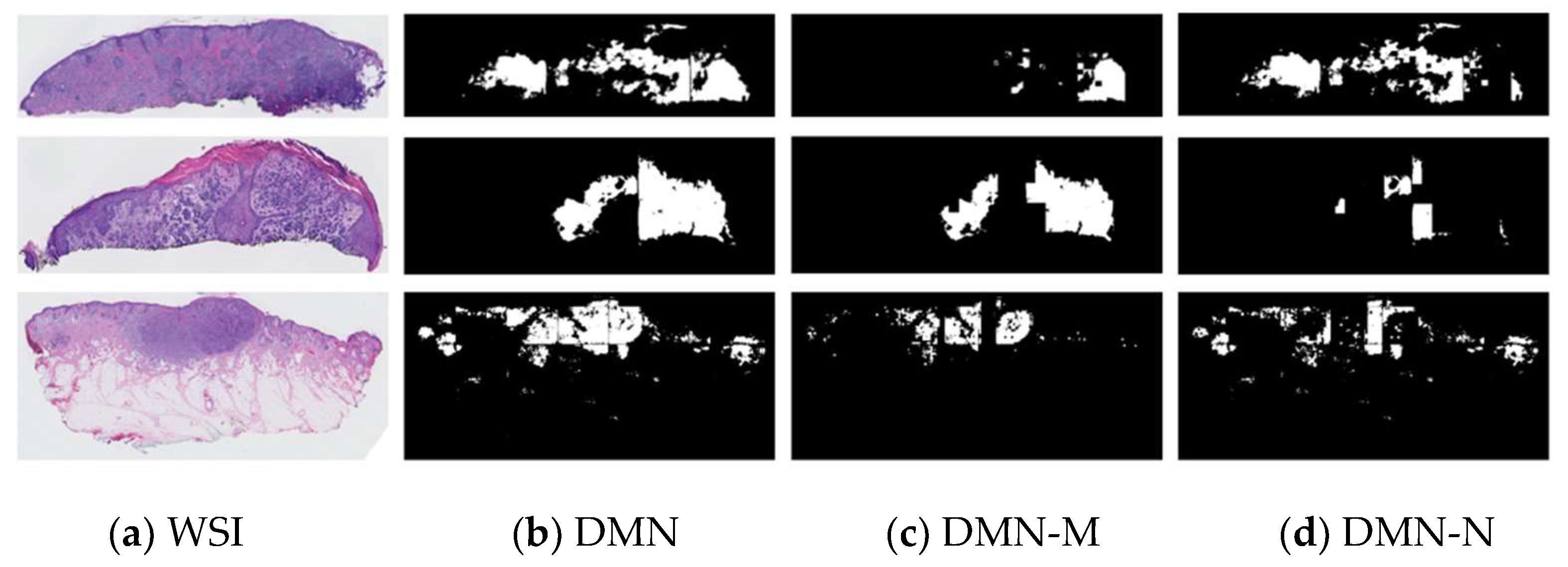
Figure 9.
Examples of our best nest classifier, ResNet’s results on WSI: (a) extracted slices of invasive melanoma WSIs; (b) dermal nest results of segmentation model; (c) melanoma dermal nest (DMN-M) portion of DMN; (d) nevus dermal nest (DMN-N) portion of DMN.
Figure 9.
Examples of our best nest classifier, ResNet’s results on WSI: (a) extracted slices of invasive melanoma WSIs; (b) dermal nest results of segmentation model; (c) melanoma dermal nest (DMN-M) portion of DMN; (d) nevus dermal nest (DMN-N) portion of DMN.
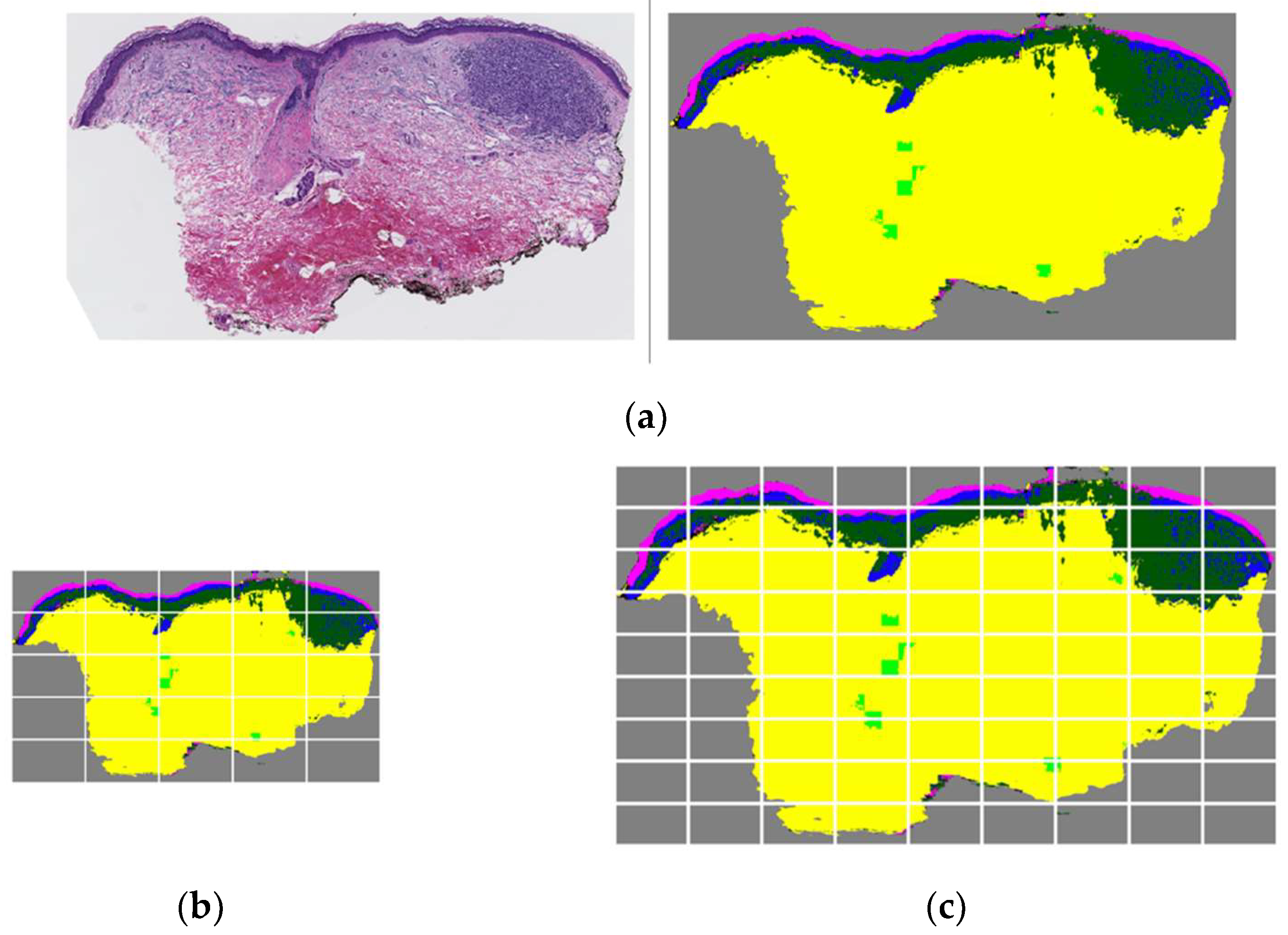
Figure 10.
Low-resolution vs. high-resolution patching when there is an inaccurate segmentation mask in the testing case. (a) A WSI and corresponding segmentation mask that includes dermis, epidermis, melanoma dermal nest, epidermal nest, corneum, and background. In this example case, epidermal nests are inaccurately segmented and over-labeled. (b) The segmentation mask in 7.5× scale divided into 25 crops as input patches for ScATNet. (c) The segmentation mask in 12.5× scale divided into 81 crops as input patches for ScATNet. There is a higher number of patches with inaccurate and noisy segmentation on the 12.5× scale compared to the 7.5× scale, which possibly led to a false prediction on the 12.5× scale using ScATNet.
Table 1.
Distribution of diagnostic categories in M-Path data.
Table 1.
Distribution of diagnostic categories in M-Path data.
| Diagnostic Category | Number of Cases |
|---|
| Class I (e.g., Mildly Dysplastic Nevi) | 25 |
| Class II (e.g., Moderately Dysplastic Nevi) | 36 |
| Class III (e.g., Melanoma in Situ) | 60 |
| Class IV (e.g., Invasive Melanoma Stage T1a) | 72 |
| Class V (e.g., Invasive Melanoma Stage ≥ T1b) | 47 |
| Total | 240 |
Table 2.
Quantitative nest classification results on ROIs-CNN models.
Table 2.
Quantitative nest classification results on ROIs-CNN models.
| Method | F-Score | Precision | Sensitivity | Specificity |
|---|
| DenseNet | 0.88 | 0.87 | 0.89 | 0.82 |
| ShuffleNet | 0.78 | 0.80 | 0.76 | 0.74 |
| ResNet | 0.96 | 0.95 | 0.97 | 0.93 |
Table 3.
Experimental results of WSI diagnosis along with segmentation masks.
Table 3.
Experimental results of WSI diagnosis along with segmentation masks.
| Experiments | F-Score * | Sensitivity ** | Specificity ** |
|---|
| Average | Min | Max | Median |
|---|
| WSI + EPN + DMN-M | 0.60 | 0.58 | 0.63 | 0.59 | 0.60 | 0.87 |
| WSI + EPN + DMN | 0.57 | 0.54 | 0.61 | 0.56 | 0.57 | 0.85 |
| WSI + EPN + DMN-M + DMN-N | 0.56 | 0.53 | 0.60 | 0.55 | 0.56 | 0.85 |
| WSI + EP + DE + EPN + DMN | 0.55 | 0.53 | 0.59 | 0.54 | 0.55 | 0.85 |
| WSI | 0.54 | 0.53 | 0.58 | 0.54 | 0.54 | 0.85 |
| WSI + EPN | 0.54 | 0.52 | 0.58 | 0.53 | 0.54 | 0.85 |
| WSI + DMN | 0.54 | 0.51 | 0.56 | 0.54 | 0.54 | 0.85 |
| WSI + DMN-M + DMN-N | 0.54 | 0.52 | 0.55 | 0.54 | 0.54 | 0.86 |
| WSI + DMN-M | 0.52 | 0.50 | 0.55 | 0.51 | 0.52 | 0.84 |
Table 4.
Comparison of two confusion matrices. Rows are defined by expert consensus and columns are by model predictions. (a) An example experiment with only WSI and no segmentation mask. (b) An example experiment of WSI + EPN + DMN-M.
Table 4.
Comparison of two confusion matrices. Rows are defined by expert consensus and columns are by model predictions. (a) An example experiment with only WSI and no segmentation mask. (b) An example experiment of WSI + EPN + DMN-M.
| | MMD | MIS | T1a | T1b | | | MMD | MIS | T1a | T1b |
|---|
| MMD | 17 | 8 | 4 | 0 | | MMD | 17 | 9 | 3 | 0 |
| MIS | 7 | 12 | 9 | 2 | | MIS | 3 | 16 | 10 | 1 |
| T1a | 0 | 9 | 18 | 4 | | T1a | 5 | 2 | 18 | 4 |
| T1b | 0 | 2 | 9 | 12 | | T1b | 0 | 0 | 8 | 15 |
| (a) WSI | | (b) WSI + EPN + DMN-M |
Table 5.
Comparison of F-score results of raw WSI and tissue experiment (WSI + EPN + DMN-M) on single-scale experiments and multi-scale experiments.
Table 5.
Comparison of F-score results of raw WSI and tissue experiment (WSI + EPN + DMN-M) on single-scale experiments and multi-scale experiments.
| Scale | WSI | WSI + EPN + DMN-M |
|---|
| 7.5× | 0.54 | 0.60 |
| 12.5× | 0.56 | 0.57 |
| 7.5× & 12.5× | 0.57 | 0.56 |
| 7.5× & 10× & 12.5× | 0.57 | 0.55 |
Table 6.
Comparison of class-based F-score, sensitivity, and specificity of 187 US pathologists and our best model (WSI + EPN + DMN-M) on the same testing set.
Table 6.
Comparison of class-based F-score, sensitivity, and specificity of 187 US pathologists and our best model (WSI + EPN + DMN-M) on the same testing set.
| Class | F-Score | Sensitivity | Specificity |
|---|
| Pathologists | Ours | Pathologists | Ours | Pathologists | Ours |
|---|
| MMD | 0.71 | 0.67 | 0.92 | 0.76 | 0.76 | 0.81 |
| MIS | 0.49 | 0.50 | 0.46 | 0.44 | 0.85 | 0.89 |
| T1a | 0.62 | 0.57 | 0.51 | 0.64 | 0.95 | 0.79 |
| T1b | 0.72 | 0.67 | 0.78 | 0.57 | 0.97 | 0.96 |
Table 7.
Comparison of baseline methods with our best model (WSI + EPN + DMN-M).
Table 7.
Comparison of baseline methods with our best model (WSI + EPN + DMN-M).
| Method | F-Score | Sensitivity | Specificity |
|---|
| penultimate-weighted [9] | 0.44 | 0.44 | 0.81 |
| hypercolumn-weighted [9] | 0.43 | 0.43 | 0.81 |
| DSMIL [10] | 0.50 | 0.50 | 0.83 |
| ChikonMIL [11] | 0.56 | 0.56 | 0.85 |
| Ours * | 0.60 | 0.60 | 0.87 |


 ,
, 


