
Analysis of Risk Factors in Patients with Subclinical Atherosclerosis and Increased Cardiovascular Risk Using Factor Analysis


Abstract
:1. Introduction
2. Related Work
3. Background of the Data Collection, Overview of Data and Data Preprocessing
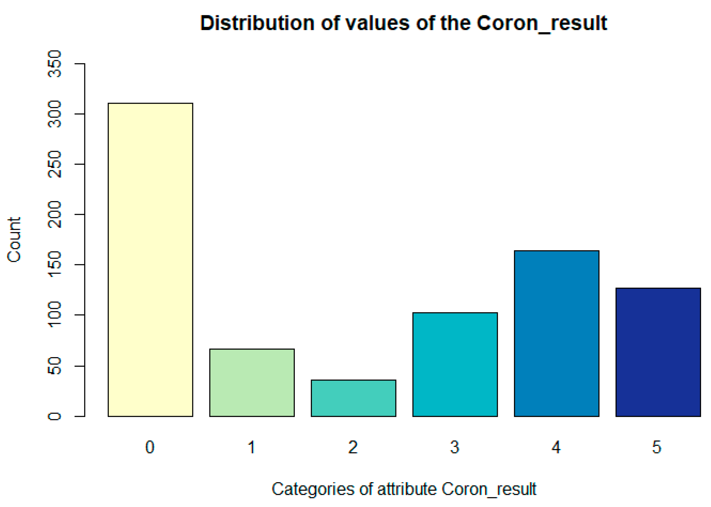
- 0—no finding;
- 1—at least one branch contains 10% narrowing;
- 2—any branch, except the RIA basin, has 20 to 50% stenosis;
- 3—RIA branches have 20 to 50% narrowing, the other 50 to 70% narrowing;
- 4—RIA branches have a maximum of 70% narrowing (50–70%), the other 70–100%;
- 5—at least one of the RIA branches has more than 70%.
Data Preprocessing
4. Methods—Factor Analysis
- Reduction of the number of attributes to reduce the computational time in data processing;
- Detection of the structure of connections hidden in the data.
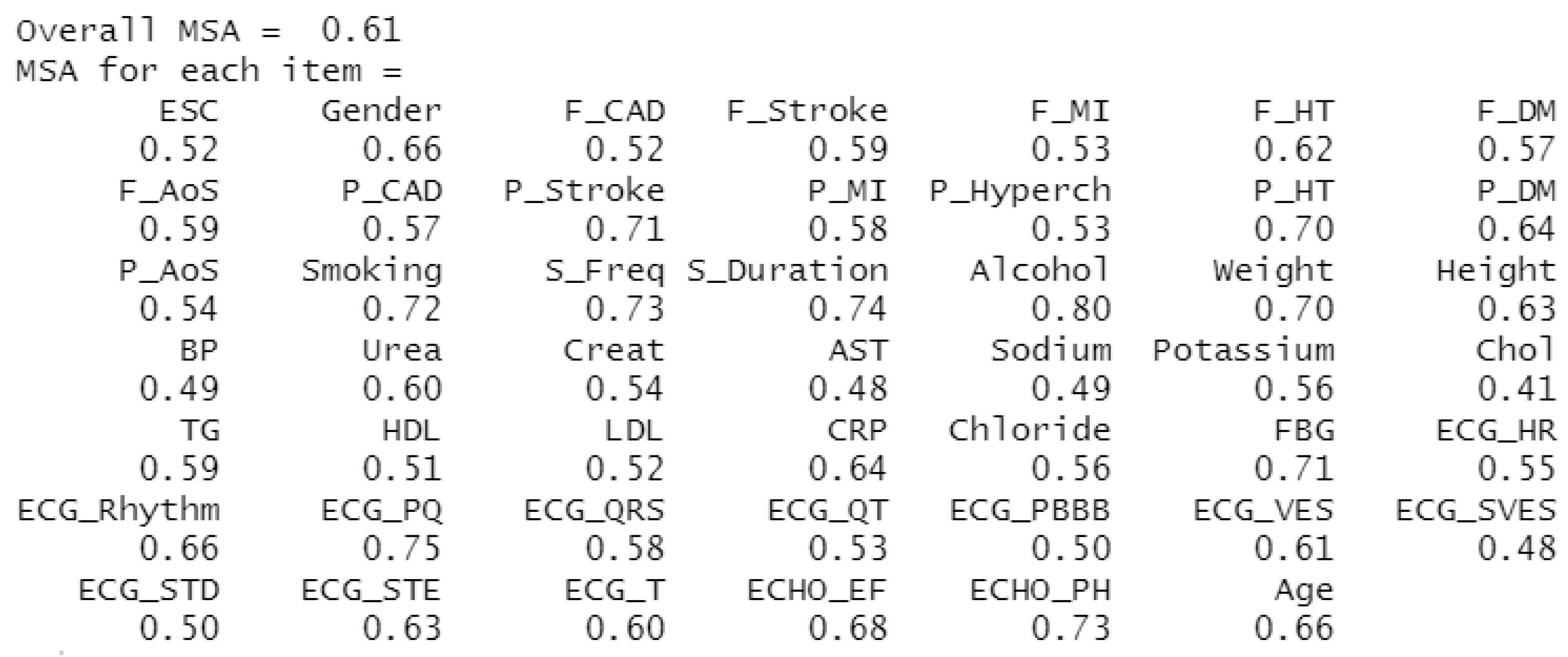
4.1. Evaluation of the Suitability of Using FA on a Selected Dataset
4.2. Determination of the Approximate Number of Factors
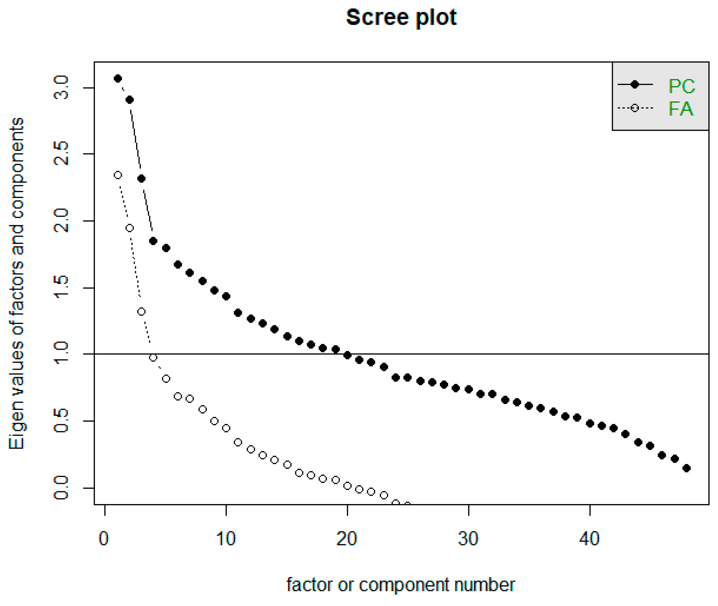
4.2.1. Scree Test
4.2.2. Kaiser Criterion
- Empirical Kaiser Criterion suggests 23 factors.
- Traditional Kaiser Criterion suggests 19 factors.
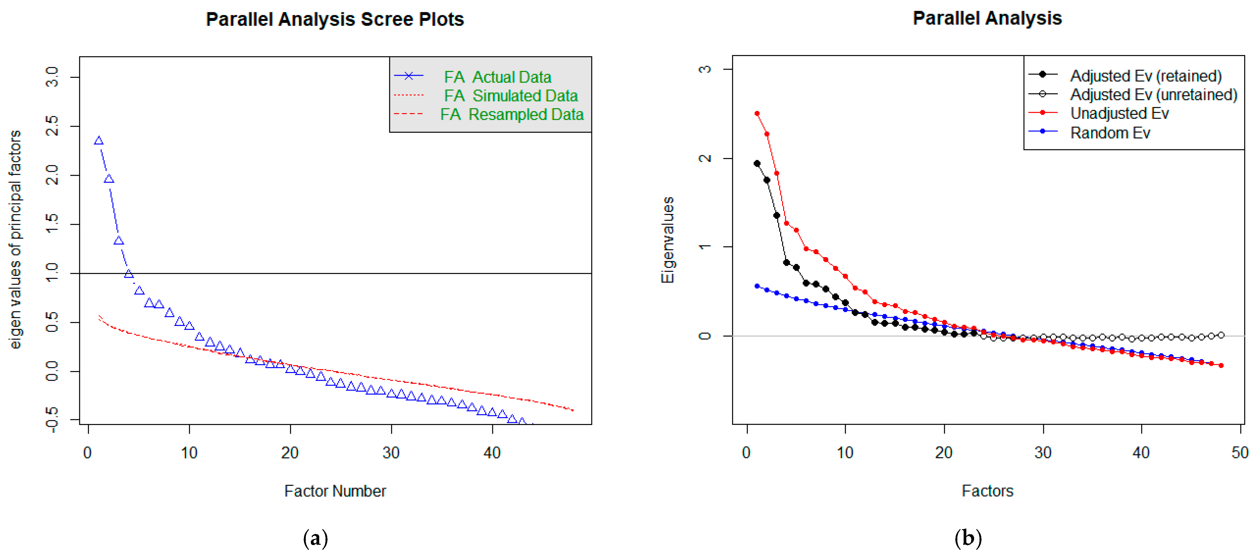
4.2.3. Parallel Analysis
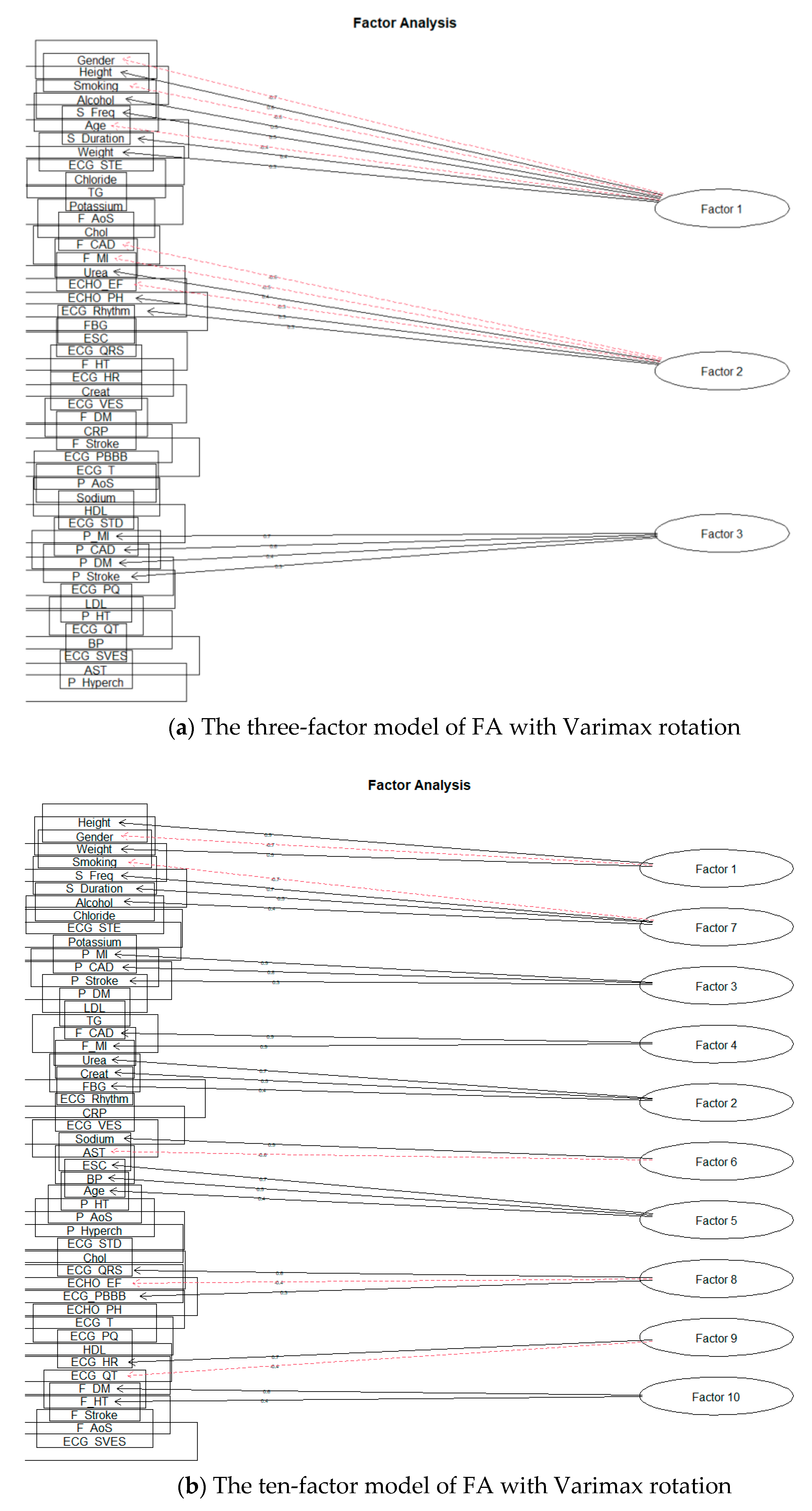
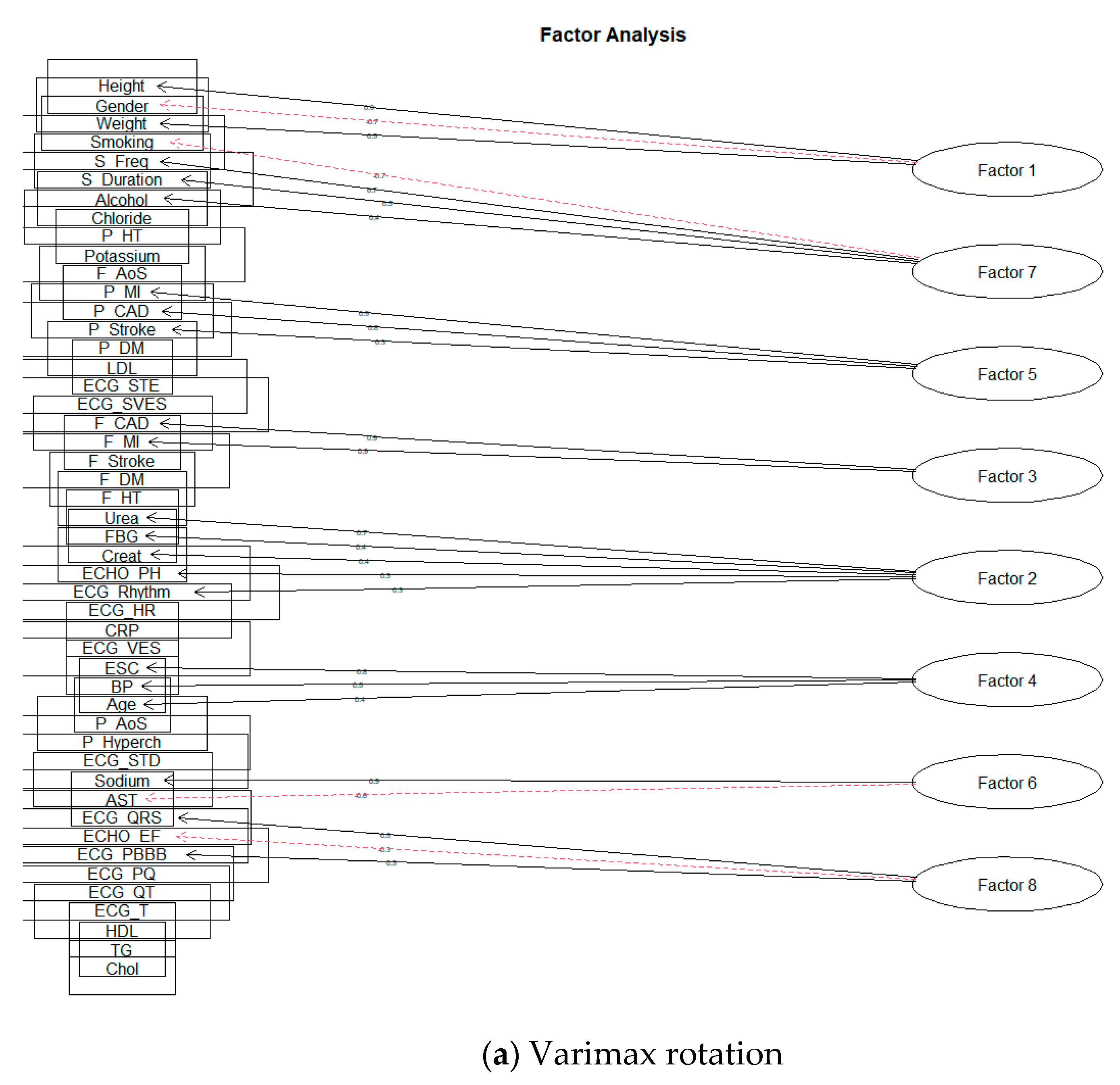
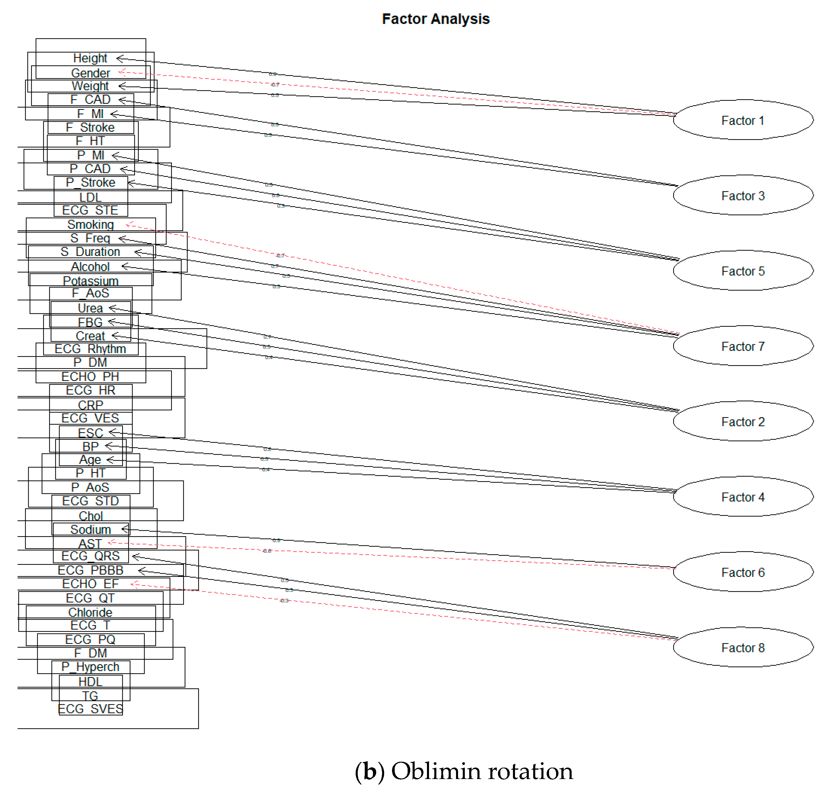
4.3. Factor Rotation
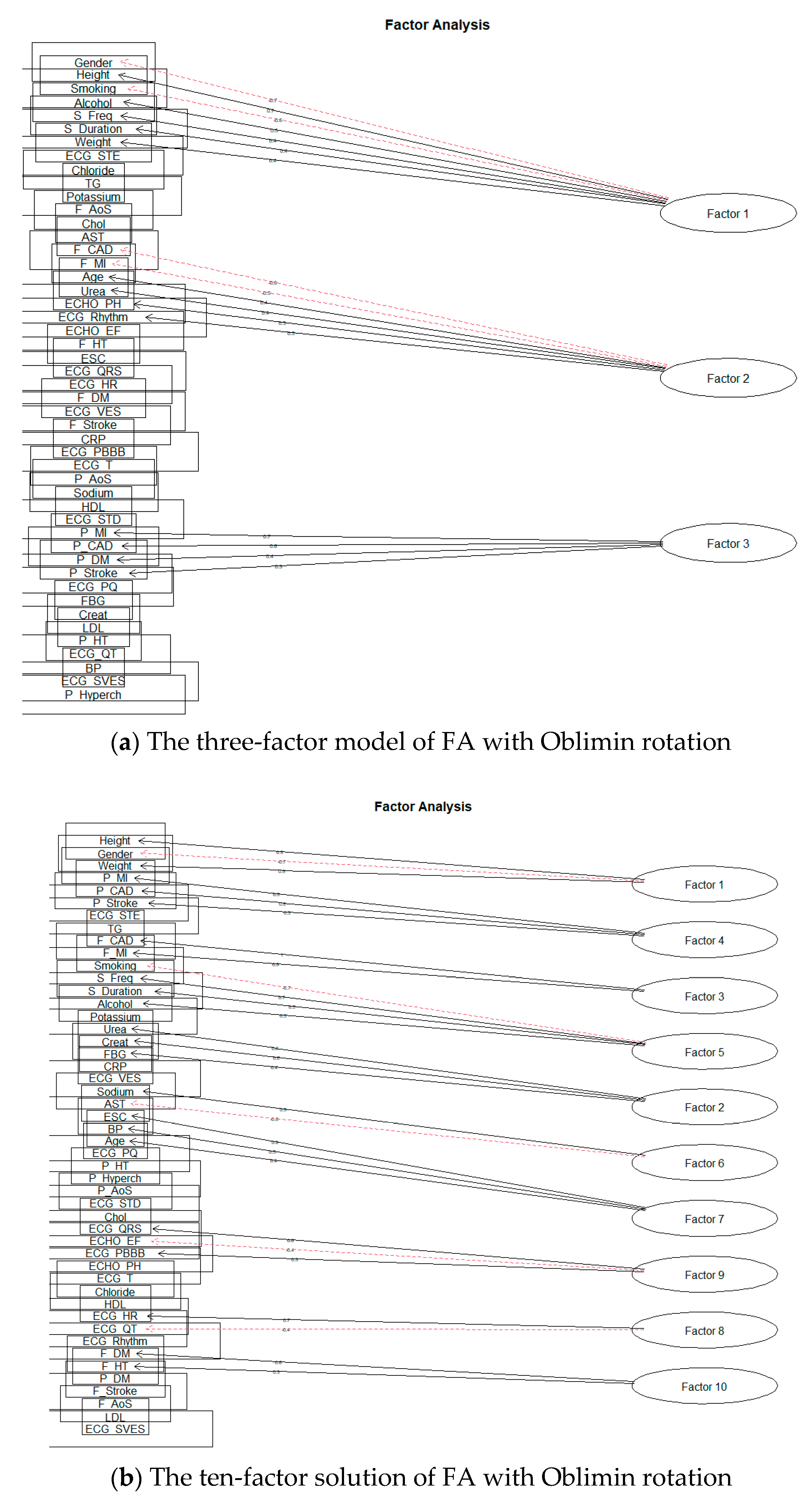
4.4. Factor Analysis Modeling
- Scree plot: 3 factors;
- Kaiser criterion: 17 factors;
- Parallel analysis: 11 factors.
4.5. Interpretation of Factor Analysis Results
4.6. Limitations of Our Study
5. Discussion
6. Conclusions
Author Contributions
Funding
Institutional Review Board Statement
Informed Consent Statement
Data Availability Statement
Conflicts of Interest
References
- De Backer, G.; Jankowski, P.; Kotseva, K.; Mirrakhimov, E.; Reiner, Ž.; Rydén, L.; Tokgözoğlu, L.; Wood, D.; De Bacquer, D.; De Backer, G.; et al. Management of dyslipidemia in patients with coronary heart disease: Results from the ESC-EORP EU-ROASPIRE V survey in 27 countries. Atherosclerosis 2019, 285, 135–146. [Google Scholar] [CrossRef] [PubMed] [Green Version]
- NCD Risk Factor Collaboration (NCD-RisC). Worldwide trends in diabetes since 1980: A pooled analysis of 751 population-based studies with 4.4 million participants. Lancet 2016, 387, 1513–1530. [Google Scholar] [CrossRef] [Green Version]
- Nolte, K.; Herrmann-Lingen, C.; Platschek, L.; Holzendorf, V.; Pilz, S.; Tomaschitz, A.; Düngen, H.D.; Angermann, C.E.; Hasenfuß, G.; Pieske, B.; et al. Vitamin D deficiency in patients with diastolic dysfunction or heart failure with preserved ejection fraction. ESC Heart Fail. 2019, 6, 262–270. [Google Scholar] [CrossRef]
- Knapik, P.; Knapik, M.; Trejnowska, E.; Kłaczek, B.; Śmietanka, K.; Cieśla, D.; Krzych Łukasz, J.; Kucewicz, E.M. Should we admit more patients not requiring invasive ventilation to reduce excess mortality in Polish intensive care units? Data from the Silesian ICU Registry. Arch. Med. Sci. 2019, 15, 1313–1320. [Google Scholar] [CrossRef]
- Pella, Z.; Milkovič, P.; Paralič, J. Application for Text Processing of Cardiology Medical Records. In Proceedings of the World Symposium on Digital Intelligence for Systems and Machines (DISA), Košice, Slovakia, 23–25 August 2018; IEEE: Danver, CO, USA, 2018; pp. 169–174. [Google Scholar]
- Dramburg, S.; Fernández, M.M.; Potapova, E.; Matricardi, P.M. The Potential of Clinical Decision Support Systems for Prevention, Diagnosis, and Monitoring of Allergic Diseases. Front. Immunol. 2020, 11, 2116. [Google Scholar] [CrossRef] [PubMed]
- Gurupur, V.; Wan, T.T.H. Inherent Bias in Artificial Intelligence-Based Decision Support Systems for Healthcare. Medicina 2020, 56, 141–154. [Google Scholar] [CrossRef] [PubMed] [Green Version]
- Tsai, T.Y.; Hsu, P.-F.; Lin, C.C.; Wang, Y.J.; Ding, Y.Z.; Liou, T.L.; Wang, Y.W.; Huang, S.S.; Chan, W.L.; Lin, S.J.; et al. Factor analysis for the clustering of cardiometabolic risk factors and sedentary behavior, a cross-sectional study. PLoS ONE 2020, 15, e242365. [Google Scholar]
- Tsai, C.H.; Li, T.C.; Lin, C.C.; Tsay, H.S. Factor analysis of modifiable cardiovascular risk factors and prevalence of metabolic syndrome in adult Taiwanese. Endocrine 2011, 40, 256–264. [Google Scholar] [CrossRef] [PubMed]
- Stoner, L.; Weatherall, M.; Skidmore, P.; Castro, N.; Lark, S.; Faulkner, J.; Williams, M.A. Cardiometabolic Risk Variables in Preadolescent Children: A Factor Analysis. JAHA 2017, 6, E007071. [Google Scholar] [CrossRef] [PubMed]
- Kaku, H.; Funakoshi, K.; Ide, T.; Fujino, T.; Matsushima, S.; Ohtani, K.; Higo, T.; Nakai, M.; Sumita, Y.; Nishimura, K.; et al. Impact of Hospital Practice Factors on Mortality in Patients Hospitalized for Heart Failure in Japan—An Analysis of a Large Number of Health Records From a Nationwide Claims-Based Database, the JROAD-DPC. Circulation 2020, 84, 742–753. [Google Scholar] [CrossRef] [PubMed]
- Pella, D.; Toth, S.; Paralic, J.; Gonsorcik, J.; Fedacko, J.; Jarcuska, P.; Pella, D.; Pella, Z.; Sabol, F.; Jankajova, M.; et al. The possible role of machine learning in detection of increased cardiovascular risk patients–KSC MR Study (design). Arch. Med. Sci. 2020. [Google Scholar] [CrossRef]
- Rousan, T.A.; Thadani, U. Stable Angina Medical Therapy Management Guidelines: A Critical Review of Guidelines from the European Society of Cardiology and National Institute for Health and Care Excellence. Eur. Cardiol. 2019, 14, 18–22. [Google Scholar] [CrossRef] [PubMed] [Green Version]
- Yadav, M.L.; Roychoudhury, B. Handling missing values: A study of popular imputation packages in R. Knowl. Based Syst. 2018, 160, 104–118. [Google Scholar] [CrossRef]
- Holzinger, K.J.; Harman, H.H. Chapter XIII: Factor Analysis. Rev. Educ. Res. 1939, 9, 528–531. [Google Scholar] [CrossRef]
- Gorunescu, F. Data Mining: Concepts, Models and Techniques; Intelligent Systems Reference Library; Springer: Berlin/Heidelberg, Germany, 2011; Volume 12, pp. 130–133. [Google Scholar]
- Olson, D.L.; Lauhoff, G. Descriptive Data Mining, 2nd ed.; Springer Nature Singapore Pte Ltd.: Singapore, 2019; p. 78. [Google Scholar]
- Wang, H.-F.; Kuo, C.-Y. Factor Analysis in Data Mining. Comput. Math. Appl. 2004, 48, 1765–1778. [Google Scholar] [CrossRef]
- Meloun, M.; Militký, J.; Hill, M. Statistická Analýza Vícerozměrných dat v Příkladech, 1st ed.; Univerzita Karlova-Karolinum: Praha, Czech Republic, 2017; pp. 110–160. [Google Scholar]
- Stankovičová, I.; Vojtková, M. Viacrozmerné Štatistické Metódy s Aplikáciami; Iura Edition: Bratislava, Slovakia, 2007. [Google Scholar]
- Coussement, K.; Demoulin, N.; Charry, K. Marketing Research with SAS Enterprise Guide, 1st ed.; Routledge: Milton Park, Abingdon, Oxfordshire, UK, 2011; pp. 69–95. [Google Scholar]
- Williams, B.; Brown, T.; Onsman, A. Exploratory factor analysis: A five-step guide for novice. JEPHC 2010, 8, 1–14. [Google Scholar] [CrossRef] [Green Version]
- Smyth, R.; Johnson, A. Factor Analysis. Western University, Faculty of Health Sciences, Test Construction. Available online: https://www.uwo.ca/fhs/tc/labs/10.FactorAnalysis.pdf (accessed on 21 May 2021).
- Kaiser, H.F. The Application of Electronic Computers to Factor Analysis. Educ. Psychol. Meas. 1960, 20, 141–151. [Google Scholar] [CrossRef]
- Goldberg, L.R.; Velicer, W.F. Principles of Exploratory Factor Analysis. In Differentiating Normal and Abnormal Personality, 2nd ed.; Strack, S., Ed.; Springer Publishing Company: New York, NY, USA, 2006; pp. 209–237. [Google Scholar]
- Osborne, J.W. What is Rotating in Exploratory Factor Analysis? PARE 2015, 20, 2. [Google Scholar]
- IBM. SPSS Statistics: Factor Analysis Rotation. Available online: https://www.ibm.com/docs/en/spss-statistics/24.0.0?topic=analysis-factor-rotation (accessed on 21 May 2021).
- Kim, J.O.; Mueller, C.W. Introduction to Factor Analysis: What It Is and How to Do It; Sage: Beverly Hills, CA, USA, 1978; p. 5. [Google Scholar]
- Kline, P. An Easy Guide to Factor Analysis, 1st ed.; Routledge: London, UK, 2002; pp. 52–53. [Google Scholar]
- Ford, C. Getting Started with Factor Analysis; University of Virginia Library: Charlottesville, VA, USA, 2016; Available online: https://data.library.virginia.edu/getting-started-with-factor-analysis/ (accessed on 23 May 2021).
- Pieters, M.; Wolberg, A.S. Fibrinogen and fibrin: An illustrated review. RPTH 2019, 3, 161–172. [Google Scholar] [CrossRef] [Green Version]
- D’Agostino, R.B., Sr.; Vasan, R.S.; Pencina, M.J.; Wolf, P.A.; Cobain, M.; Massaro, J.M.; Kannel, W.B. General cardiovascular risk profile for use in primary care: The Framingham Heart Study. Circulation 2008, 117, 743–753. [Google Scholar] [CrossRef] [PubMed] [Green Version]
- McClelland, R.L.; Chung, H.; Detrano, R.; Post, W.; Kronmal, R.A. Distribution of coronary artery calcium by race, gender, and age: Results from the Multi-Ethnic Study of Atherosclerosis (MESA). Circulation 2006, 113, 30–37. [Google Scholar] [CrossRef] [Green Version]
- Vikram, N.K.; Pandey, R.M.; Misra, A.; Goel, K.; Gupta, N. Factor analysis of the metabolic syndrome components in urban Asian Indian adolescents. Asia Pac. J. Clin. Nutr. 2009, 18, 293–300. [Google Scholar] [PubMed]
- Hobkirk, J.P.; King, R.F.; Gately, P.; Pemberton, P.; Smith, A.; Barth, J.H.; Carroll, S. Longitudinal factor analysis reveals a distinct clustering of cardiometabolic improvements during intensive, short-term dietary and exercise intervention in obese children and adolescents. Metab. Syndr. Relat. Disord. 2012, 10, 20–25. [Google Scholar] [CrossRef]
- Lafortuna, C.L.; Adorni, F.; Agosti, F.; Sartorio, A. Factor analysis of metabolic syndrome components in obese woman. Nutr. Metab. Cardiovasc Dis. 2008, 18, 233–241. [Google Scholar] [CrossRef] [PubMed]
- Gupta, J.; Mitra, N.; Kanetsky, P.A.; Devaney, J.; Wing, M.R.; Reilly, M.; Shah, V.O.; Balakrishnan, V.S.; Guzman, N.J.; Girndt, M.; et al. Association between albuminuria, kidney function, and inflammatory biomarker profile in CKD in CRIC. Clin. J. Am. Soc. Nephrol. 2012, 7, 1938–1946. [Google Scholar] [CrossRef] [Green Version]
- Marušič, A. Factor analysis of risk for coronary heart disease: An independent replication. Int. J. Cardiol. 2000, 75, 233–238. [Google Scholar] [CrossRef]
- Goodman, E.; Dolan, L.M.; Morrison, J.A.; Daniels, S.R. Factor analysis of clustered cardiovascular risks in adolescence: Obesity is the predominant correlate of risk among youth. Circulation 2005, 111, 1970–1977. [Google Scholar] [CrossRef] [PubMed] [Green Version]
- Collingwood, T.R.; Bernstein, I.H.; Blair, S.N. The Interrelation of Coronary Heart Disease Risk Factors: A Factor Analysis of 23 Variables. J. Cardiopulm. Rehabil. 1987, 7, 234–238. [Google Scholar] [CrossRef]
- Mayer-Davis, E.J.; Ma, B.; Lawson, A.; D’Agostino, R.B.; Liese, A.D.; Bell, R.A.; Dabelea, D.; Dolan, L.; Pettitt, D.J.; Rodriguez, B.L.; et al. Cardiovascular disease risk factors in youth with type 1 and type 2 diabetes: Implications of a factor analysis of clustering. Metab. Syndr. Relat. Disord. 2009, 7, 89–95. [Google Scholar] [CrossRef] [PubMed] [Green Version]
- Pedrosa, R.B.S.; Rodrigues, R.C.M.; Padilha, K.M.; Gallani, M.C.B.J.; Alexandre, N.M.C. Factor analysis of an instrument to measure the impact of disease on daily life. Rev. Bras. Enferm. 2016, 69, 650–657. [Google Scholar]
- Hagan, R.D.; Parrish, G.; Licciardone, J.C. Physical Fitness Is Inversely Related to Heart Disease Risk: A Factor Analytical Study. Am. J. Prev. Med. 1991, 7, 237–243. [Google Scholar] [CrossRef]
- Piotrowski, G.; Szymański, P.; Banach, M.; Piotrowska, A.; Gawor, R.; Rysz, J.; Gawor, Z. Left atrial and left atrial appendage systolic function in patients with post-myocardial distal blocks. Arch. Med. Sci. 2010, 6, 895–899. [Google Scholar] [CrossRef] [PubMed]


| Attribute | Type | Description | Values |
|---|---|---|---|
| Identifying attributes | |||
| Id | numeric | according to a medical report | - |
| BN | text | encrypted birth number | - |
| Year | numeric | year of birth of the patient | min: 1930; mean: 1952.06; sd: 9.36; median: 1952; max: 1982; IQR: 13 |
| Gender | binary | patient’s gender | 0 (male): 460; 1 (female): 348 |
| Symptomatic attributes | |||
| P_CAD | binary | personal ischemic heart disease | FALSE: 478; TRUE: 329; NA: 1 |
| P_Stroke | binary | personal stroke | FALSE: 703; TRUE: 104; NA: 1 |
| P_MI | binary | personal infarct myocardium | FALSE: 591; TRUE: 216; NA: 1 |
| P_Hyperch | binary | personal disease associated with high-level cholesterol | FALSE: 748; TRUE: 59; NA: 1 |
| P_HT | binary | personal high blood pressure | FALSE: 264; TRUE: 543; NA: 1 |
| P_DM | binary | personal type 2 diabetes | FALSE: 570; TRUE: 237; NA: 1 |
| P_AoS | binary | personal aortic stenosis | FALSE: 738; TRUE: 69; NA: 1 |
| F_CAD | binary | ischemic heart disease—occurrence in family | FALSE: 616; TRUE: 185; NA: 7 |
| F_Stroke | binary | stroke—occurrence in family | FALSE: 702; TRUE: 104; NA: 7 |
| F_MI | binary | infarct myocardium—occurrence in family | FALSE: 655; TRUE: 146; NA: 7 |
| F_Hyperch | binary | disease associated with high-level cholesterol—occurrence in family | FALSE: 801; NA: 7 |
| F_HT | binary | high blood pressure—occurrence in family | FALSE: 735; TRUE: 66; NA: 7 |
| F_DM | binary | type 2 diabetes—occurrence in family | FALSE: 570; TRUE: 237; NA: 7 |
| F_AoS | binary | aortic stenosis—occurrence in family | FALSE: 800; TRUE: 1; NA: 7 |
| Smoking | categorical | type of smoker | 1 (smoker): 100; 2 (ex-smoker): 140; 3 (non-smoker): 489; NA: 79 |
| S_Duration | numeric | number of years of smoking | min: 0; mean: 2.79; sd: 8.43; median: 0; max: 60; IQR: 0; NA: 79 |
| S_Freq | numeric | number of daily smoked cigarettes | min: 0; mean: 2.21; sd: 6.24; median: 0; max: 60; IQR: 0; NA: 79 |
| Alcohol | binary | alcohol consumption | FALSE: 488; TRUE: 127, NA: 193 |
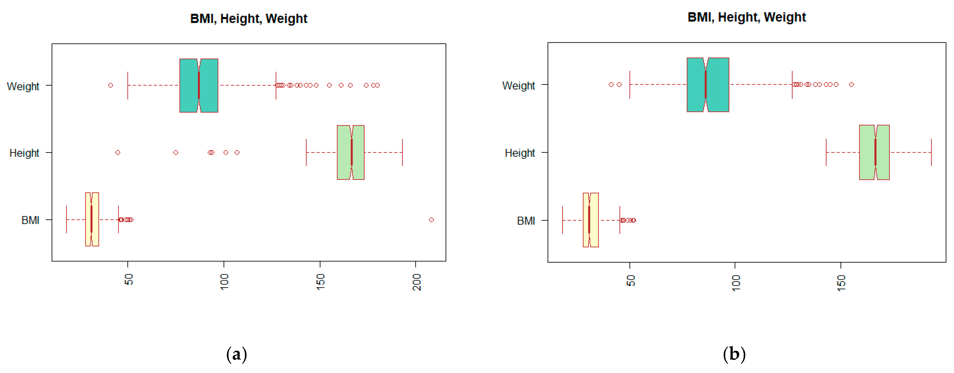
| Weight | numeric | patient weight | min: 41; mean: 88; sd: 17.96; median: 88; max: 180; IQR: 20; NA: 27 |
| Height | numeric | patient height | min: 45; mean: 165.74; sd: 11.65; median: 166; max: 193; IQR: 14; NA: 27 |
| BMI | numeric | body mass index | min: 18.22; mean: 31.84; sd: 8.3; median: 31; max: 208.12; IQR: 7; NA: 27 |
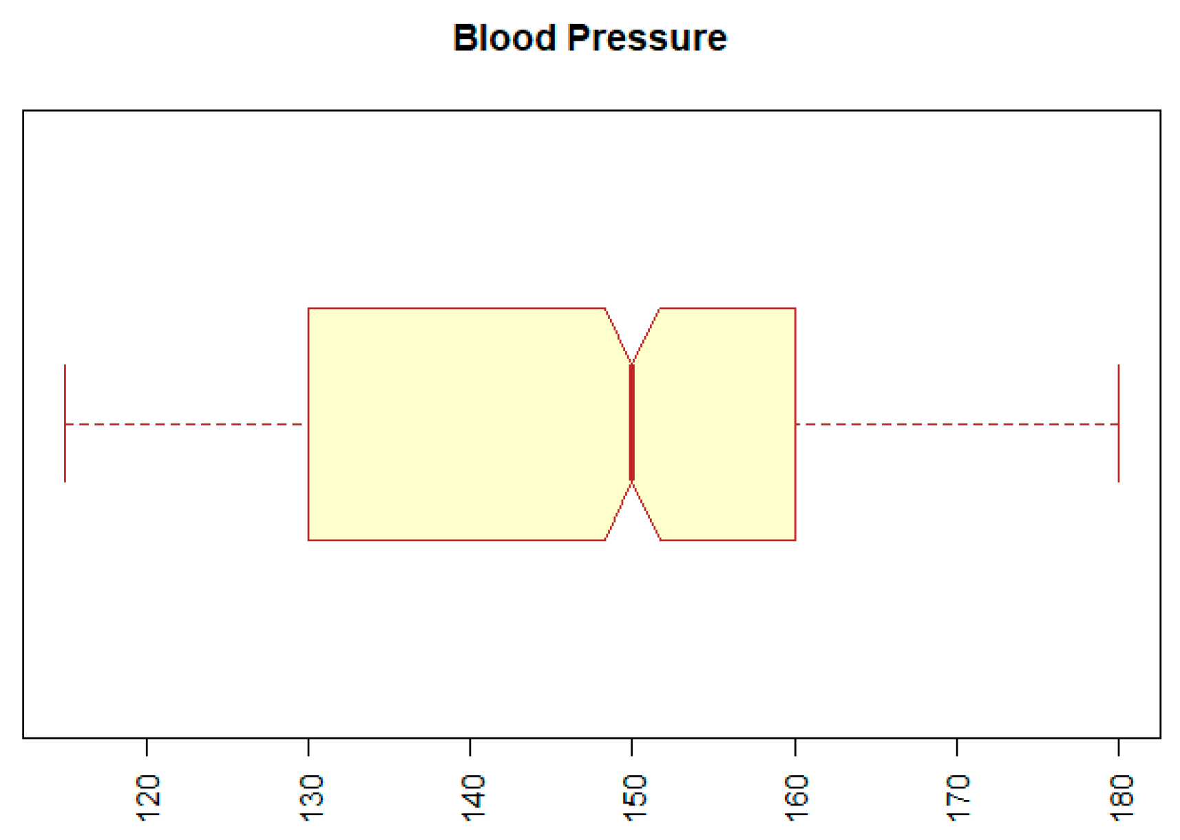
| BP | numeric | blood pressure | min: 12; mean: 167.91; sd: 510.18; median: 150; max: 14090; IQR: 30; NA: 54 |
| Urea | numeric | blood urea level | min: 2.29; mean: 6.29; sd: 2.66; median: 5.69; max: 27.13; IQR: 2.42; NA: 26 |
| Creat | numeric | blood creatinine level | min: 6.6; mean: 87.83; sd: 50.17; median: 80.4; max: 735.2; IQR: 25.53; NA: 14 |
| AST | numeric | the level of enzyme secreted by the liver | min: 0.08; mean: 0.73; sd: 6.27; median: 0.38; max: 141; IQR: 0.16; NA: 303 |
| Sodium | numeric | blood sodium level | min: 4.4; mean: 138.8; sd: 8.56; median: 139; max: 169.7; IQR: 3.75; NA: 7 |
| Potassium | numeric | blood potassium level | min: 2.9; mean: 4.33; sd: 1.99; median: 4.26; max: 58.45; IQR: 0.70; NA: 18 |
| Chol | numeric | total cholesterol | min: 0.82; mean: 5.78; sd: 22.03; median: 4.81; max: 614; IQR: 1.67; NA: 39 |
| TG | numeric | level of triacylglycerols | min: 0.46; mean: 1.79; sd: 1.72; median: 1.41; max: 30.01; IQR: 0.91; NA: 59 |
| HDL | numeric | high-density lipoprotein level | min: 0.51; mean: 1.47; sd: 3.93; median: 1.27; max: 108; IQR: 0.45; NA: 62 |
| LDL | numeric | low-density lipoprotein level | min: 0.89; mean: 3.07; sd: 1.06; median: 2.94; max: 9.6; IQR: 1.42; NA: 84 |
| CRP | numeric | C-reactive protein level | min: 0.1; mean: 5.86; sd: 10.88; median: 3.21; max: 130.4; IQR: 5.15; NA: 401 |
| Chloride | numeric | blood chloride level | min: 91.8; mean: 103.5; sd: 3.38; median: 103.6; max: 111.2; IQR: 3.9; NA: 695 |
| FBG | numeric | fibrinogen levels | min: 2.1; mean: 3.91; sd: 1.06; median: 3.7; max: 7.4; IQR: 1.25; NA: 661 |
| HIV | binary | the presence of HIV | FALSE: 627; NA: 181 |
| HBsAG | binary | the presence of an antigen evoking the presence of jaundice type B | FALSE: 626; NA: 182 |
| ECG_HR | numeric | heart rate for minute | min: 45; mean: 69.54; sd: 12.23; median: 68; max: 130; IQR: 14; NA: 56 |
| ECG_Rhythm | binary | type of heart rhythm | 0 (SR): 704; 1(Fib): 60; NA: 44 |
| ECG_PQ | numeric | the length of the interval from the beginning of the P wave to the beginning of the ventricular complex in milliseconds | min: 14; mean: 170.2; sd: 33.08; median: 160; max: 360; IQR: 30; NA: 170 |
| ECG_QRS | numeric | heart ventricular depolarization time in milliseconds | min: 60; mean: 95.8; sd: 19.57; median: 90; max: 180; IQR: 20; NA: 117 |
| ECG_QT | numeric | time from the beginning of the QRS to the end of the T wave in milliseconds | min: 40; mean: 386.4; sd: 43.57; median: 380; max: 518; IQR: 40; NA: 249 |
| ECG_LBBB | binary | the presence of a blockage of the left Tawar arm | FALSE: 764; NA: 44 |
| ECG_RBBB | binary | the presence of a blockage of the right Tawar arm | FALSE: 696; TRUE: 68; NA: 44 |
| ECG_VES | binary | presence of ventricular extrasystoles | FALSE: 721; TRUE: 43; NA: 44 |
| ECG_SVES | binary | presence of supraventricular (atrial) extrasystoles | FALSE: 739; TRUE: 25; NA: 44 |
| ECG_STD | binary | the presence of depression in the ST segment | FALSE: 643; TRUE: 121; NA: 44 |
| ECG_STE | binary | presence of elevations in the ST section | FALSE: 529; TRUE: 235; NA: 44 |
| ECG_T | binary | ventricular myocardial repolarization | FALSE: 163; TRUE: 604; NA: 44 |
| ECHO_EF | numeric | left ventricular ejection fraction | min: 15; mean: 52.72; sd: 9.93; median: 55; max: 75; IQR: 12; NA: 39 |
| ECHO_PH | categorical | degree of pulmonary hypertension | 0: 629; 1: 78; 2: 44; 3: 56; NA: 1 |
| Resulting attributes | |||
| Muscle_bridge | binary | the presence of a muscle bridge in one of the branches | FALSE: 802; TRUE: 5; NA: 1 |
| ACS | numeric | percentage narrowing of the branch of Arteria coronaria sinistra | min: 0; mean: 6.35; sd: 19.44; median: 0; max: 100; IQR: 0; NA:1 |
| RIA | numeric | percentage narrowing of the Ramus interventricularis anterior branch | min: 0; mean: 21.73; sd: 33.18; median: 0; max: 100; IQR: 0; NA: 1 |
| RD1 | numeric | percentage narrowing of branch RD1, part of RIA | min: 0; mean: 4.83; sd: 18.35; median: 0; max: 100; IQR: 0; NA: 1 |
| RD2 | numeric | percentage narrowing of branch RD2, part of RIA | min: 0; mean: 1.24; sd: 9.35; median: 0; max: 100; IQR: 0; NA: 1 |
| RCX | numeric | percentage narrowing of the ramus circumflex artery branch | min: 0; mean: 17.18; sd: 30.86; median: 0; max: 100; IQR: 10; NA: 1 |
| RIM | numeric | percentage narrowing of the RIM branch, part of the RCX | min: 0; mean: 2.55; sd: 12.69; median: 0; max: 100; IQR: 0; NA: 1 |
| RMS1 | numeric | percentage narrowing of the RMS1 branch, part of the RCX | min: 0; mean: 5.16; sd: 18.20; median: 0; max: 100; IQR: 0; NA: 1 |
| RMS2 | numeric | percentage narrowing of the RMS2 branch, part of the RCX | min: 0; mean: 2.08; sd: 12.09; median: 0; max: 100; IQR: 0; NA: 1 |
| ACD | numeric | percentage narrowing of the Arteria coronaria dextra branch | min: 0; mean: 23.62; sd: 35.66; median: 0; max: 100; IQR: 50; NA: 1 |
| RIP | numeric | percentage narrowing of the Ramus interventricularis posterior branch | min: 0; mean: 2.78; sd: 13.58; median: 0; max: 100; IQR: 0; NA: 1 |
| Coron_result | categorical | the degree of severity of the finding | 0: 310; 1: 67; 2: 36; 3: 103; 4: 164; 5: 126 |
| Value of KMO | The Adequacy of the Observed Data Set |
|---|---|
| ≥0.9 | Excellent |
| <0.8; 0.9) | Commendable |
| <0.7; 0.8) | Moderately useful |
| <0.6; 0.7) | Average |
| <0.5; 0.6) | Weak |
| <0.5 | Not enough |
| Factors | Factor Loadings |
|---|---|
| The three-factor solution for Varimax rotation | |
| Factor 1 | Gender; Height; Smoking; Alcohol; S_Freq; Age; S_Duration |
| Factor 2 | F_CAD; F_MI; Urea; ECHO_EF; ECHO_PH; ECG_Rhythm |
| Factor 3 | P_MI; P_CAD; P_DM; P_Stroke |
| The ten-factor solution for Varimax rotation | |
| Factor 1 | Height; Gender; Weight |
| Factor 2 | Urea; Creat; FBG |
| Factor 3 | P_MI; P_CAD; P_Stroke |
| Factor 4 | F_CAD; F_MI |
| Factor 5 | ESC; BP; Age |
| Factor 6 | Sodium; AST |
| Factor 7 | Smoking; S_Freq; S_Duration; Alcohol |
| Factor 8 | ECG_QRS; ECHO_EF; ECG_RBBB; ECHO_PH |
| Factor 9 | ECG_HR; ECG_QT |
| Factor 10 | F_DM; F_HT |
| The three-factor solution for Oblimin rotation | |
| Factor 1 | Gender; Height; Smoking; Alcohol; S_Freq; S_Duration; Weight |
| Factor 2 | F_CAD; F_MI; Age; Urea; ECHO_PH; ECG_Rhythm; ECHO_EF |
| Factor 3 | P_MI; P_CAD; P_DM; P_Stroke |
| The ten-factor solution for Oblimin rotation | |
| Factor 1 | Height; Gender; Weight |
| Factor 2 | Urea; Creat; FBG |
| Factor 3 | F_CAD; F_MI |
| Factor 4 | P_MI; P_CAD; P_Stroke |
| Factor 5 | Smoking; S_Freq; S_Duration; Alcohol |
| Factor 6 | Sodium; AST |
| Factor 7 | ESC; BP; Age |
| Factor 8 | ECG_HR; ECG_QT |
| Factor 9 | ECG_QRS; ECHO_EF; ECG_RBBB |
| Factor 10 | F_DM; F_HT |
| Factors | SS Loadings | Factors | SS Loading |
|---|---|---|---|
| Factor rotation ‘Varimax’ | Factor rotation ‘Oblimin’ | ||
| The three-factor solution | |||
| Factor 1 | 2.37 | Factor 1 | 2.36 |
| Factor 2 | 1.88 | Factor 2 | 1.89 |
| Factor 3 | 1.86 | Factor 3 | 1.86 |
| The ten-factor solution | |||
| Factor 1 | 1.89 | Factor 1 | 1.96 |
| Factor 2 | 1.56 | Factor 2 | 1.49 |
| Factor 3 | 1.77 | Factor 3 | 1.75 |
| Factor 4 | 1.71 | Factor 4 | 1.77 |
| Factor 5 | 1.22 | Factor 5 | 1.76 |
| Factor 6 | 1.23 | Factor 6 | 1.23 |
| Factor 7 | 1.81 | Factor 7 | 1.23 |
| Factor 8 | 1.2 | Factor 8 | 0.98 * |
| Factor 9 | 0.96 * | Factor 9 | 1.20 |
| Factor 10 | 0.93 * | Factor 10 | 0.98 * |
| Factors | SS Loadings | Factor Loadings |
|---|---|---|
| Factor rotation ‘Varimax’ | ||
| Factor 1 | 1.87 | Height; Gender; Weight |
| Factor 2 | 1.65 | Urea; FBG; Creat; ECHO_PH; ECG_Rhythm |
| Factor 3 | 1.76 | F_CAD; F_MI |
| Factor 4 | 1.24 | ESC; BP; Age |
| Factor 5 | 1.77 | P_MI; P_CAD; P_Stroke |
| Factor 6 | 1.22 | Sodium; AST |
| Factor 7 | 1.84 | Smoking; S_Freq; S_Duration; Alcohol |
| Factor 8 | 1.10 | ECG_QRS; ECHO_EF; ECG_RBBB |
| Factor rotation ‘Oblimin’ | ||
| Factor 1 | 1.97 | Height; Gender; Weight |
| Factor 2 | 1.57 | Urea; FBG; Creat |
| Factor 3 | 1.77 | F_CAD; F_MI |
| Factor 4 | 1.25 | ESC; BP; Age |
| Factor 5 | 1.77 | P_MI; P_CAD; P_Stroke |
| Factor 6 | 1.23 | Sodium; AST |
| Factor 7 | 1.78 | Smoking; S_Freq; S_Duration; Alcohol |
| Factor 8 | 1.12 | ECG_QRS; ECG_RBBB; ECHO_EF |
| Model | Cumulative Variance |
|---|---|
| Factor rotation Varimax | |
| The three-factor solution | 13% |
| The eight-factor solution | 26% |
| Factor rotation Oblimin | |
| The three-factor solution | 13% |
| The eight-factor solution | 26% |
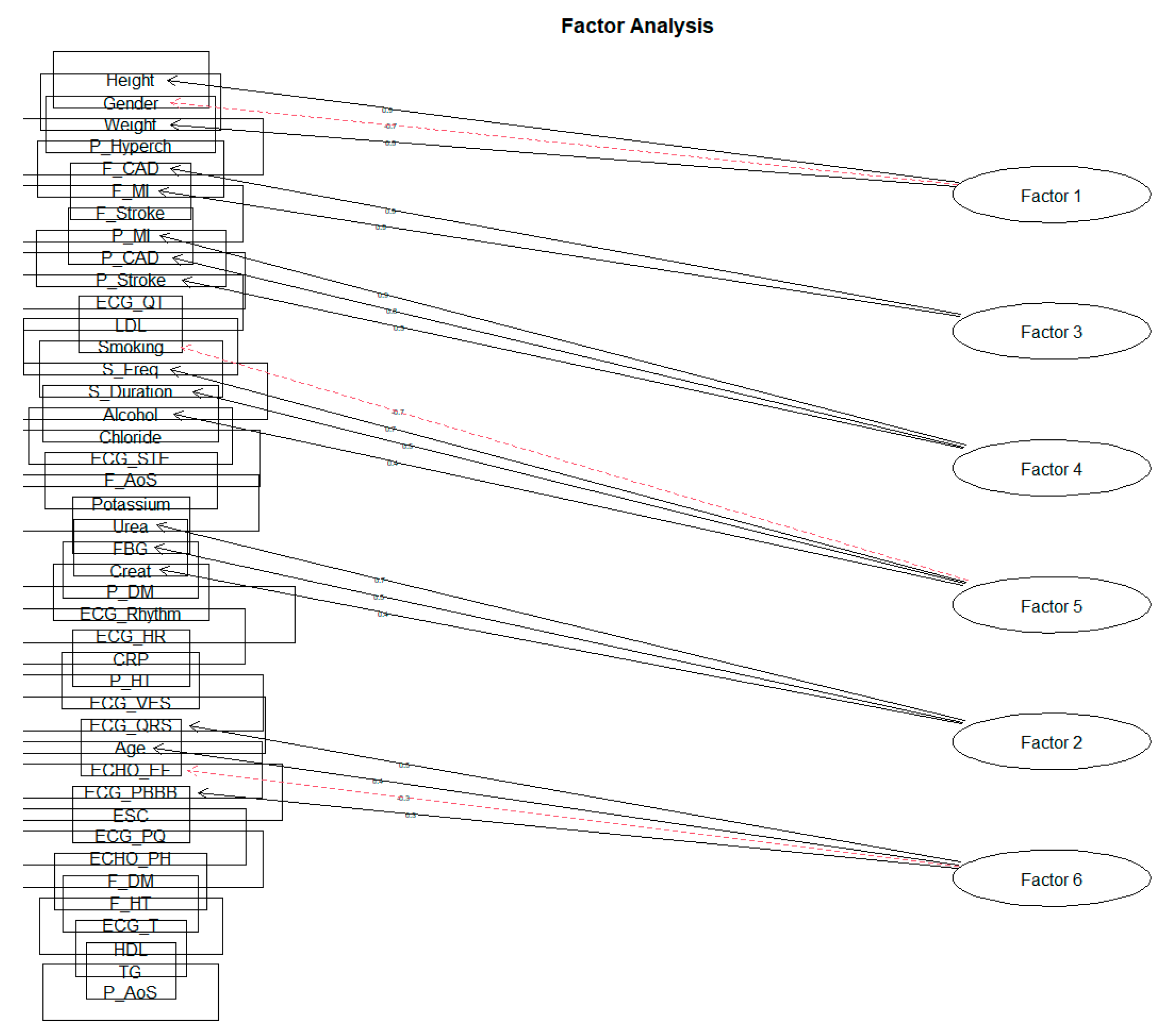
| Factors | SS Loadings | Factor Loadings |
|---|---|---|
| Factor 1 | 1.97 | Height; Gender; Weight |
| Factor 2 | 1.50 | Urea; FBG; Creat |
| Factor 3 | 1.77 | F_CAD; F_MI |
| Factor 4 | 1.75 | P_MI; P_CAD; P_Stroke |
| Factor 5 | 1.76 | Smoking; S_Freq; S_Duration; Alcohol |
| Factor 6 | 1.23 | ECG_QRS; Age; ECHO_EF; ECKG_PBBB |
| Factor 1 | Factor 2 | Factor 3 | Factor 4 | Factor 5 | Factor 6 | |
|---|---|---|---|---|---|---|
| Height | 0.890 * | −0.023 | −0.006 | −0.035 | −0.036 | −0.034 |
| Gender | −0.702 * | −0.030 | 0.013 | −0.041 | −0.166 | −0.156 |
| Weight | 0.510 * | 0.193 | −0.042 | 0.076 | −0.082 | −0.085 |
| Urea | 0.010 | 0.684 * | 0.007 | −0.044 | −0.057 | 0.028 |
| FBG | −0.012 | 0.463 * | −0.034 | 0.097 | 0.260 | −0.033 |
| Creat | 0.103 | 0.436 * | 0.027 | 0.006 | −0.037 | −0.046 |
| F_CAD | −0.015 | −0.002 | 0.912 * | −0.014 | −0.009 | 0.003 |
| F_MI | 0.004 | 0.009 | 0.896 * | 0.016 | −0.009 | 0.008 |
| P_MI | 0.016 | −0.017 | 0.027 | 0.869 * | 0.007 | 0.009 |
| P_CAD | −0.036 | −0.006 | −0.033 | 0.772 * | −0.015 | −0.007 |
| P_Stroke | −0.022 | 0.062 | −0.044 | 0.329 * | −0.007 | 0.025 |
| Smoking | −0.049 | 0.073 | 0.027 | −0.057 | −0.738 * | 0.019 |
| S_Freq | −0.029 | 0.038 | 0.014 | −0.054 | 0.652 * | −0.079 |
| S_Duration | −0.024 | 0.091 | 0.058 | −0.060 | 0.536 * | 0.075 |
| Alcohol | 0.201 | −0.062 | 0.042 | −0.079 | 0.361 * | 0.039 |
| ECG_QRS | 0.153 | −0.074 | 0.042 | 0.006 | −0.086 | 0.530 * |
| Age | −0.372 | 0.207 | −0.061 | 0.014 | −0.092 | 0.414 * |
| ECHO_EF | −0.270 | −0.162 | 0.016 | −0.092 | −0.033 | −0.309 * |
| ECG_RBBB | 0.012 | −0.046 | 0.019 | −0.041 | −0.009 | 0.309 * |
| SS loading | 1.965 | 1.499 | 1.771 | 1.753 | 1.755 | 1.230 |
| Proportion Variance | 0.047 | 0.036 | 0.042 | 0.042 | 0.042 | 0.029 |
| Cumulative Variance | 0.047 | 0.083 | 0.125 | 0.167 | 0.209 | 0.238 |
Publisher’s Note: MDPI stays neutral with regard to jurisdictional claims in published maps and institutional affiliations. |
© 2021 by the authors. Licensee MDPI, Basel, Switzerland. This article is an open access article distributed under the terms and conditions of the Creative Commons Attribution (CC BY) license (https://creativecommons.org/licenses/by/4.0/).
Share and Cite
Pella, Z.; Pella, D.; Paralič, J.; Vanko, J.I.; Fedačko, J. Analysis of Risk Factors in Patients with Subclinical Atherosclerosis and Increased Cardiovascular Risk Using Factor Analysis. Diagnostics 2021, 11, 1284. https://doi.org/10.3390/diagnostics11071284
Pella Z, Pella D, Paralič J, Vanko JI, Fedačko J. Analysis of Risk Factors in Patients with Subclinical Atherosclerosis and Increased Cardiovascular Risk Using Factor Analysis. Diagnostics. 2021; 11(7):1284. https://doi.org/10.3390/diagnostics11071284
Chicago/Turabian StylePella, Zuzana, Dominik Pella, Ján Paralič, Jakub Ivan Vanko, and Ján Fedačko. 2021. "Analysis of Risk Factors in Patients with Subclinical Atherosclerosis and Increased Cardiovascular Risk Using Factor Analysis" Diagnostics 11, no. 7: 1284. https://doi.org/10.3390/diagnostics11071284