
Conventional Machine Learning versus Deep Learning for Magnification Dependent Histopathological Breast Cancer Image Classification: A Comparative Study with Visual Explanation

 , , ,
, , ,  , ,
, ,
Abstract
:1. Introduction
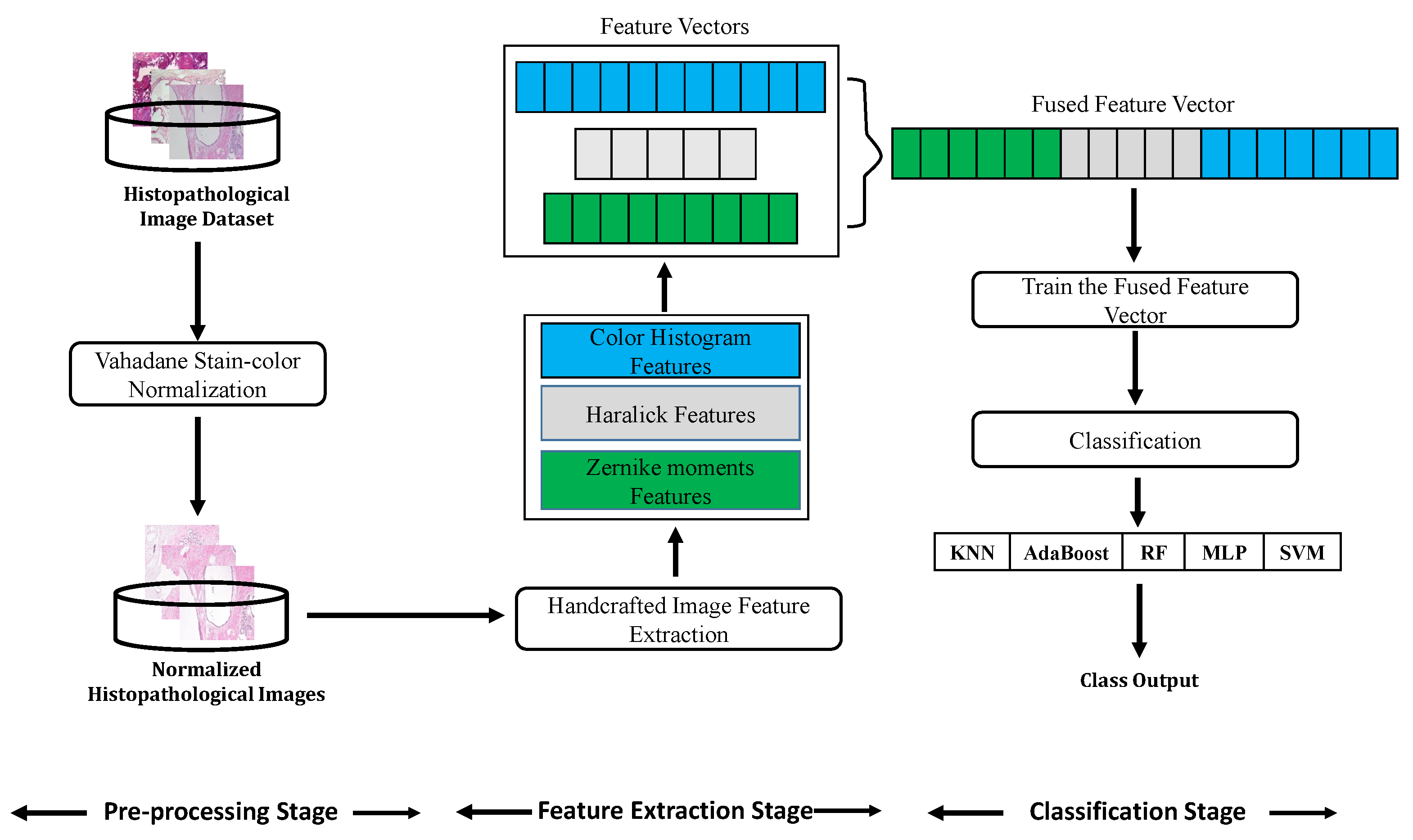
- We apply different feature extractors and classifiers to the task of histopathological BC image classification to make a full comparison. We extract handcrafted features using three feature extractor techniques (Zernike moments, Haralick, and color histogram), and the extracted feature vectors are then fused. The obtained feature vector is subsequently classified using five classical classifiers: KNN, random forest (RF), multi-layer perceptron (MLP), Adaptive Boosting (AdaBoost), and SVM.
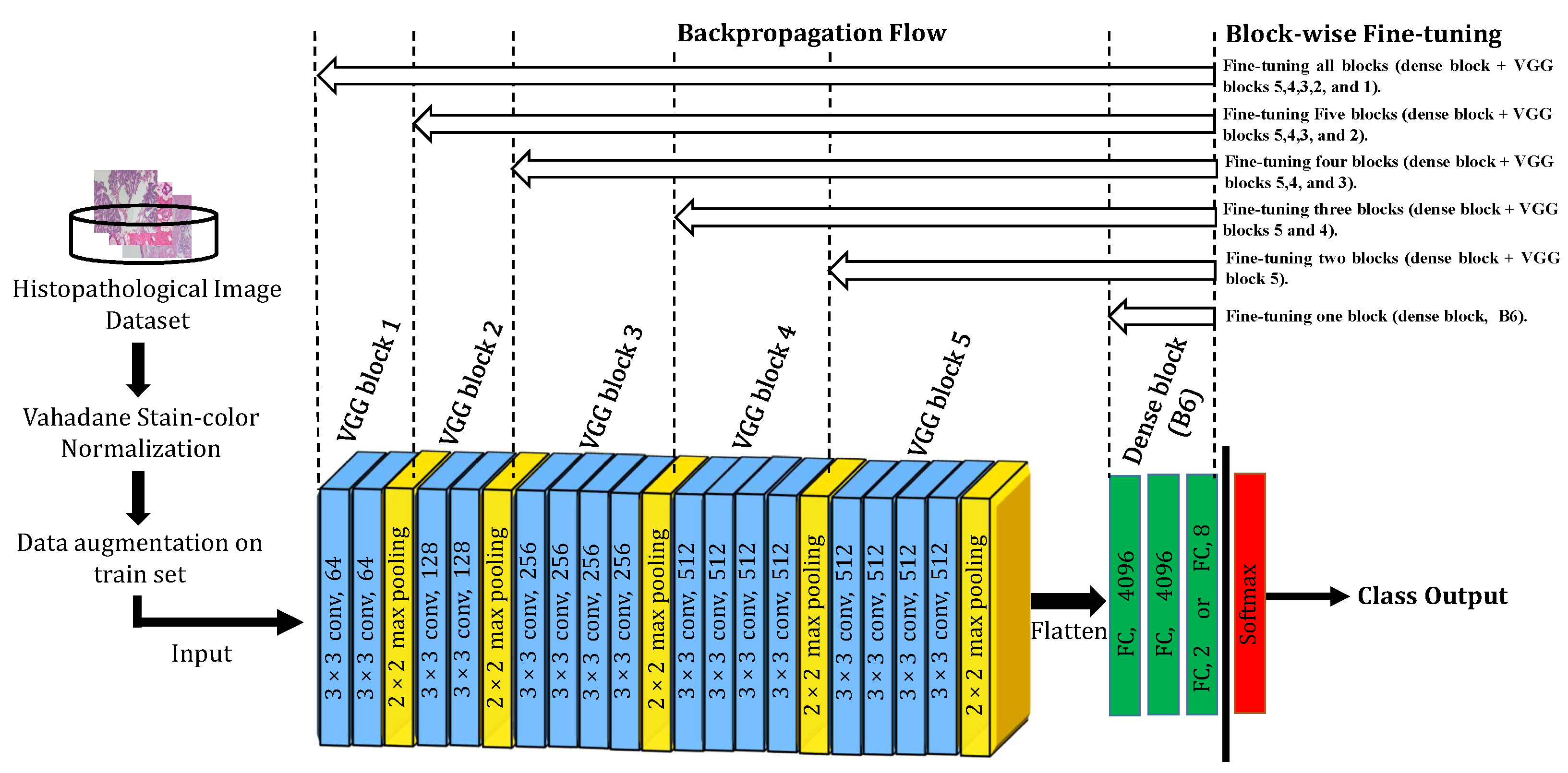
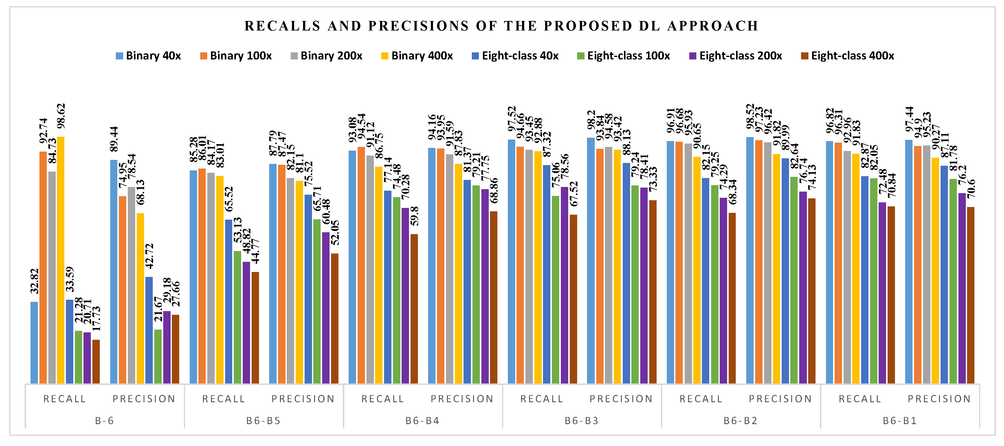
- Based on our previous work [21] where two fine-tuned residual blocks from the ImageNet pre-trained ResNet-18 model were sufficient to achieve recent state-of-the-art results for magnification dependent classification, we are motivated to investigate the block-wise fine-tuning strategy on another deep CNN architecture, VGG-19 [22]. We extend our previous work by fine-tuning VGG-19 block-by-block aiming to figure out the best proportion of blocks to fine-tune when classifying breast histopathological images with respect to their magnification factors while examining and discussing the impact of block-wise fine-tuning on the classification results.
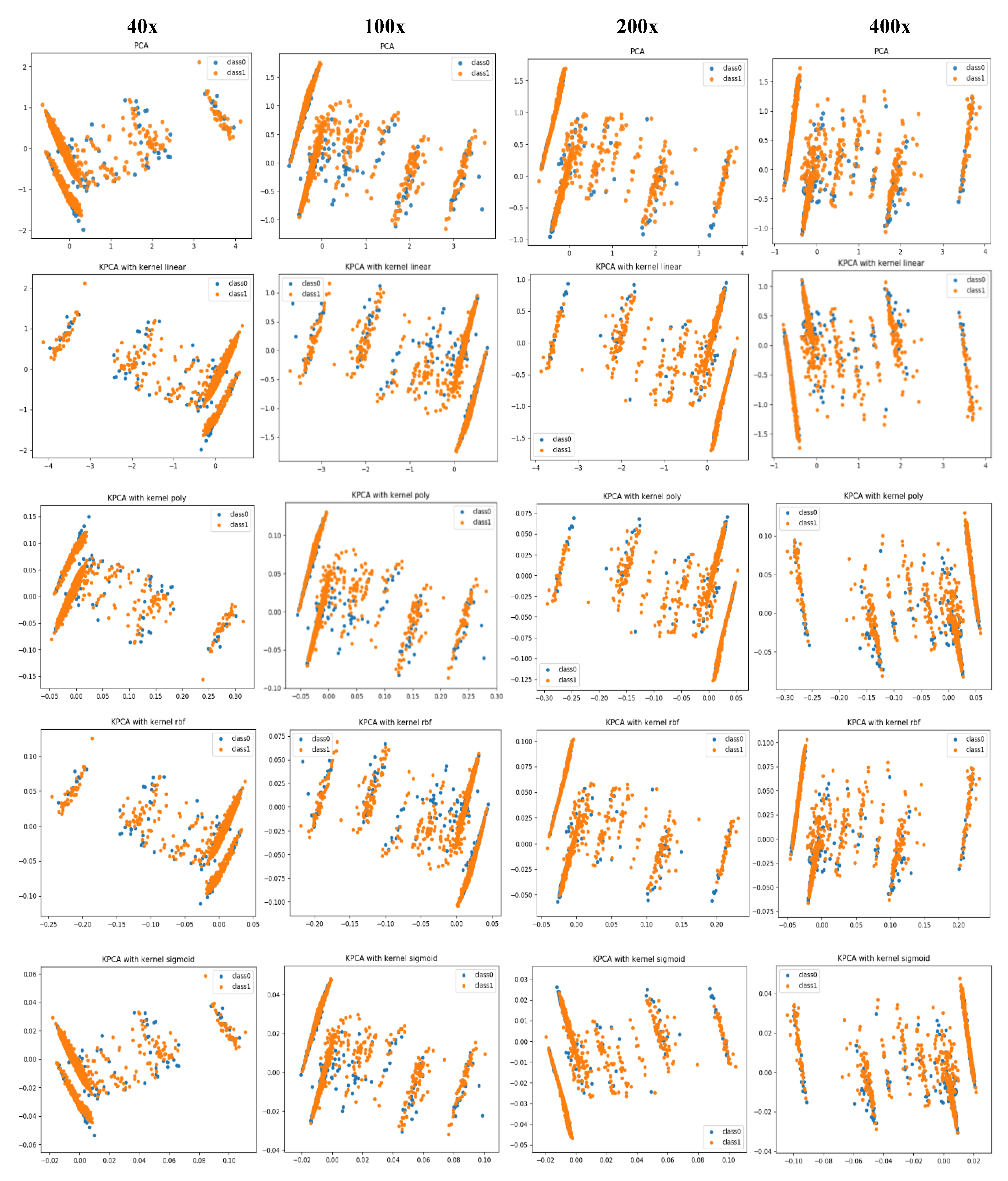
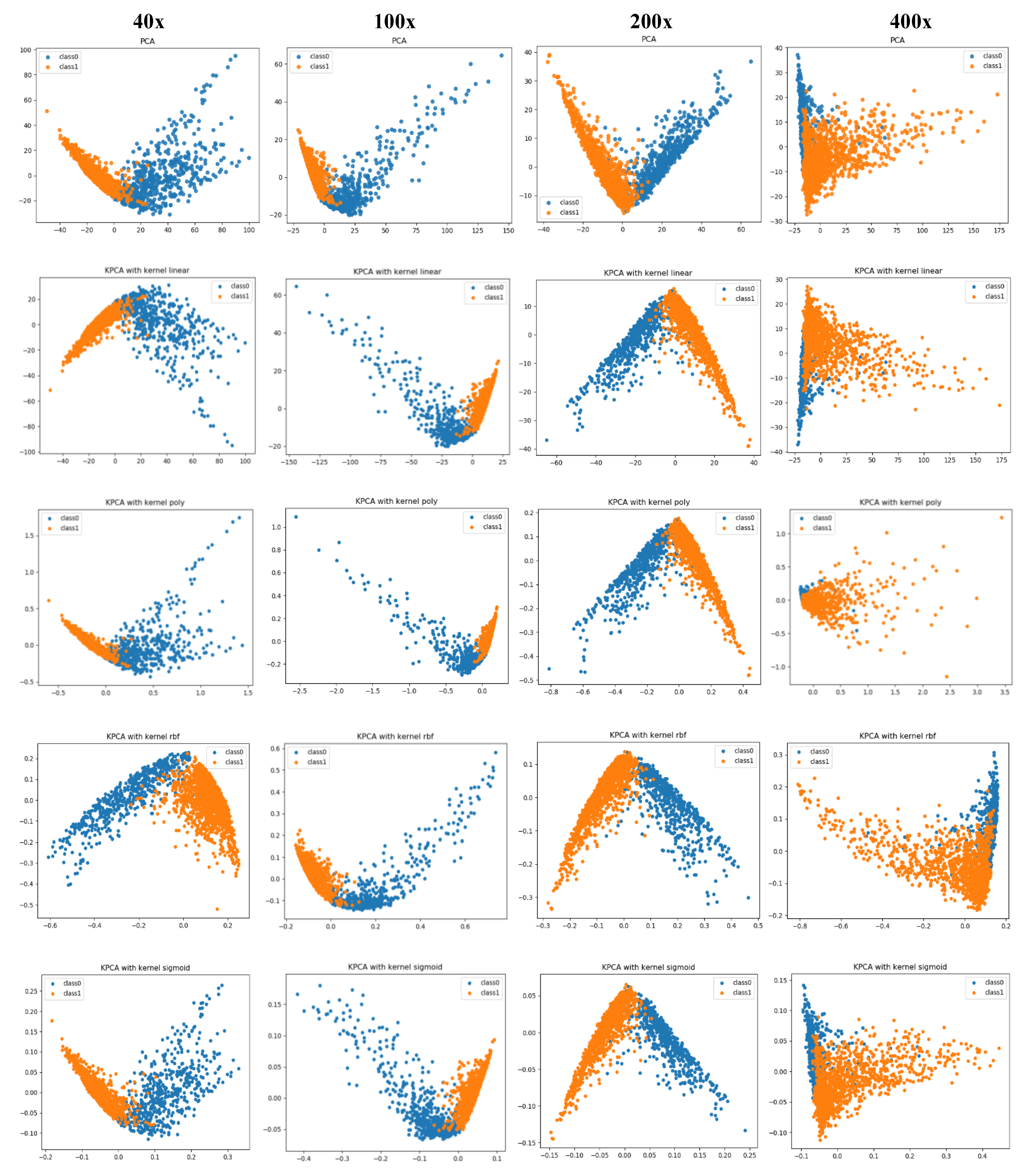
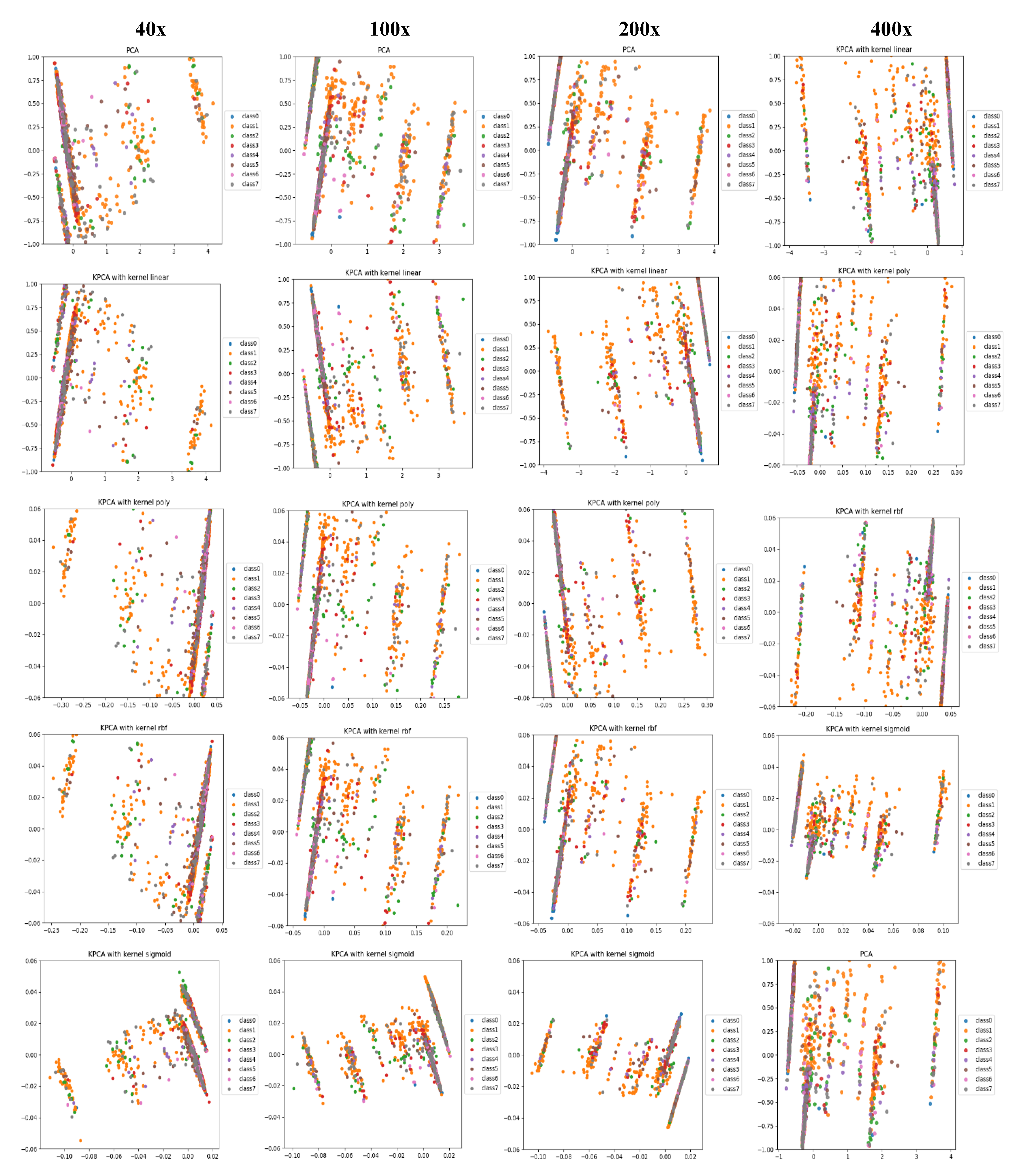
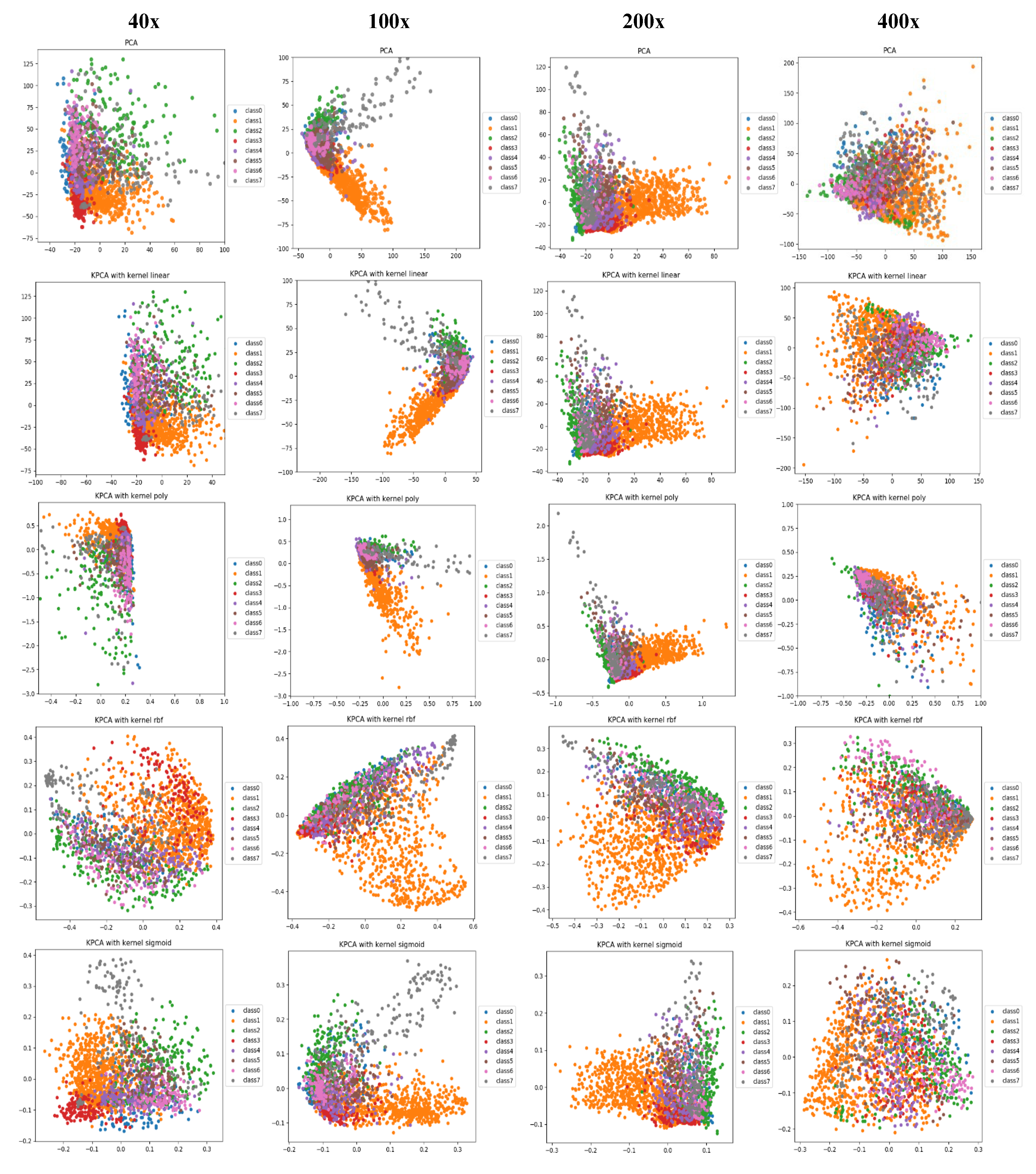
- Along with the comparison of classification performance, we provide a visual interpretation for the compared approaches. We use principal component analysis (PCA) and kernel-PCA (KPCA) to reduce the deep features and handcrafted features to 2D space and then visualize/compare them intuitively. Through the comparison of the visualization results, the difference in classification performance between CML and DL methods can be explained.
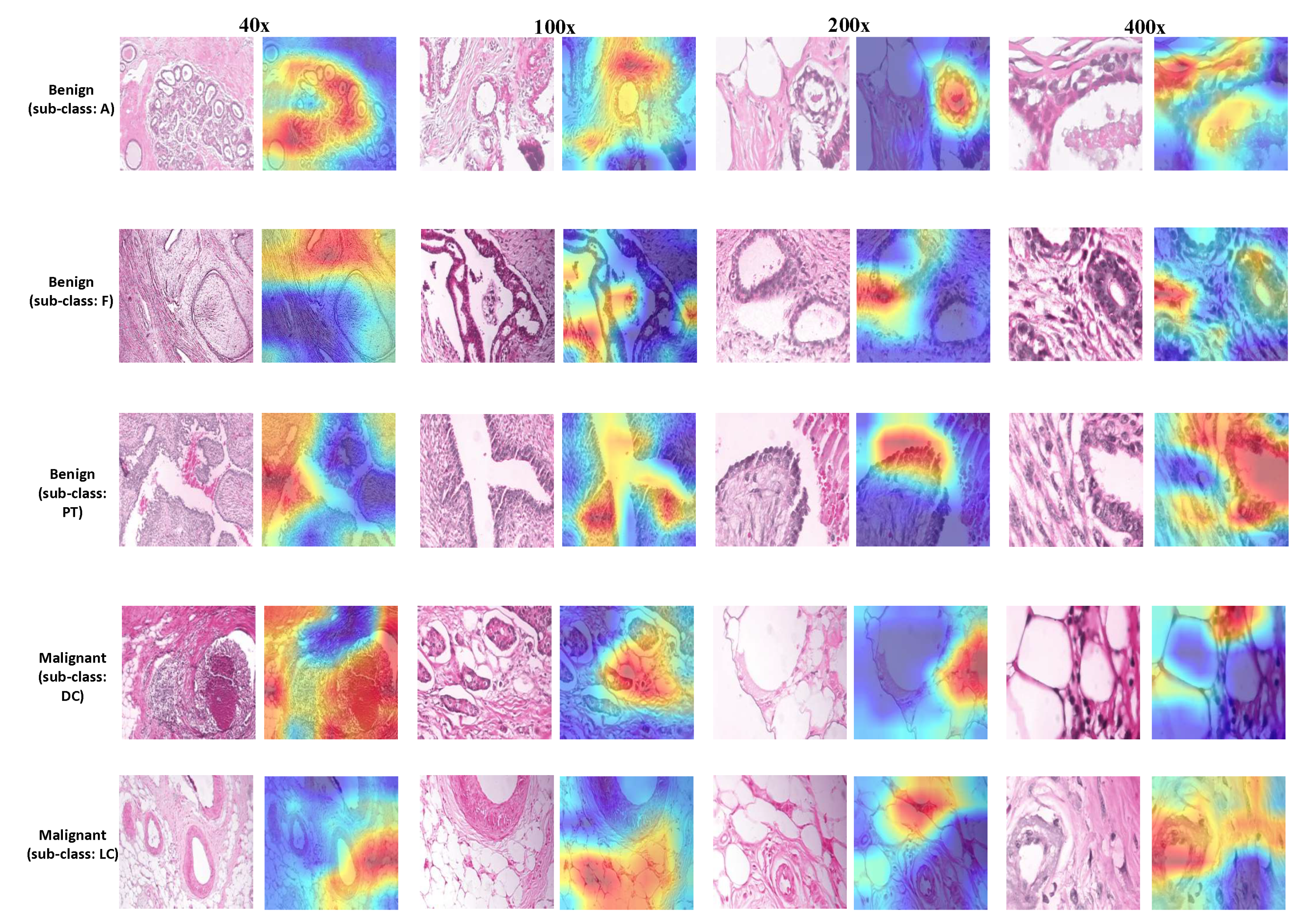
- We further explore the explanation of the diagnosis decision of the DL method. We obtain the activation map of the last convolutional layer from the DL model by Grad-CAM, and then visualize it using a heatmap, showing where in the input image (key areas), the DL models are looking to settle on a certain class output. Through the explanation, we can provide the diagnosis decision and the reasons for making such a decision simultaneously, which inherently helps to improve the pathologist’s trust in automated DL methods.
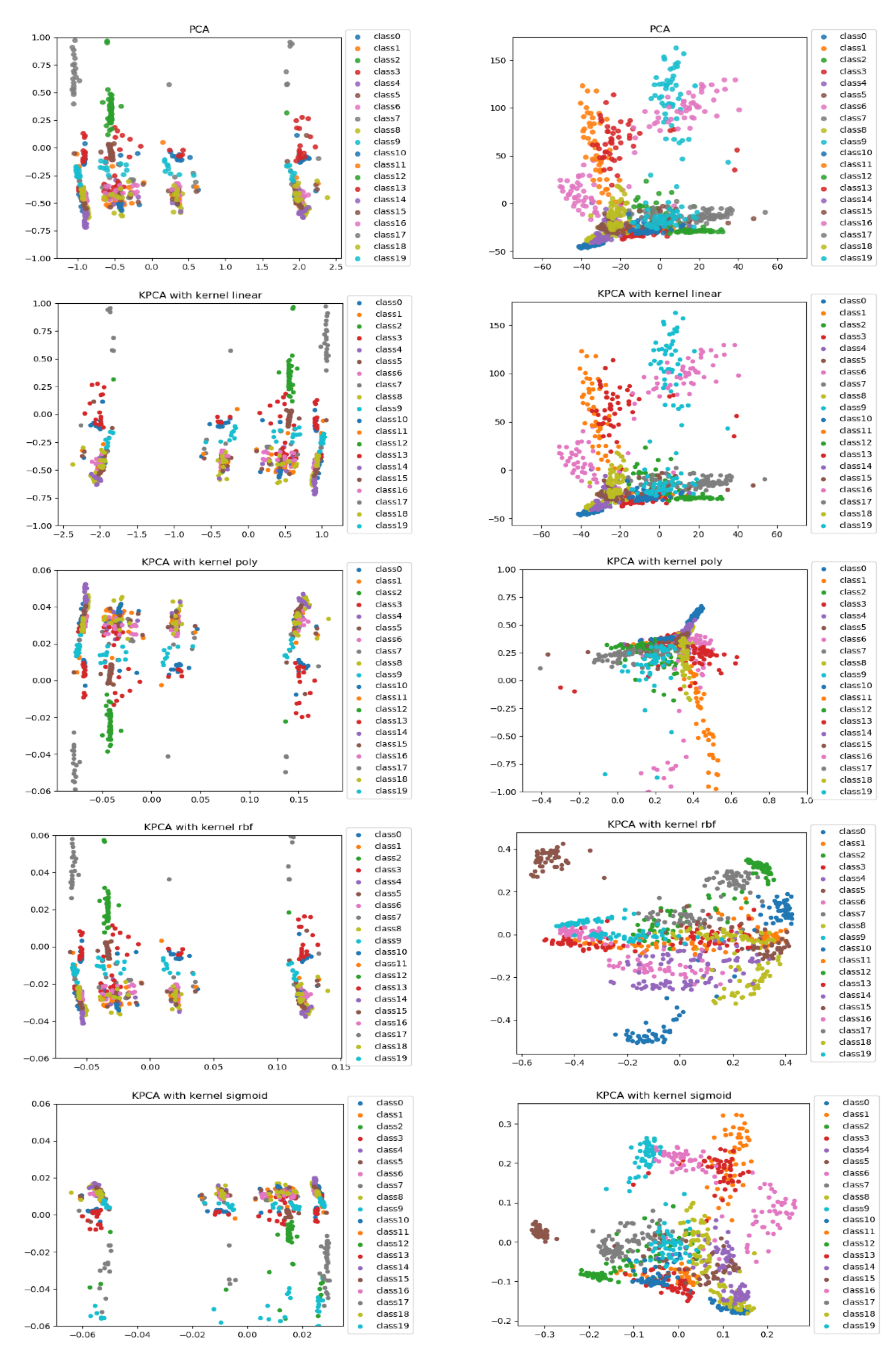
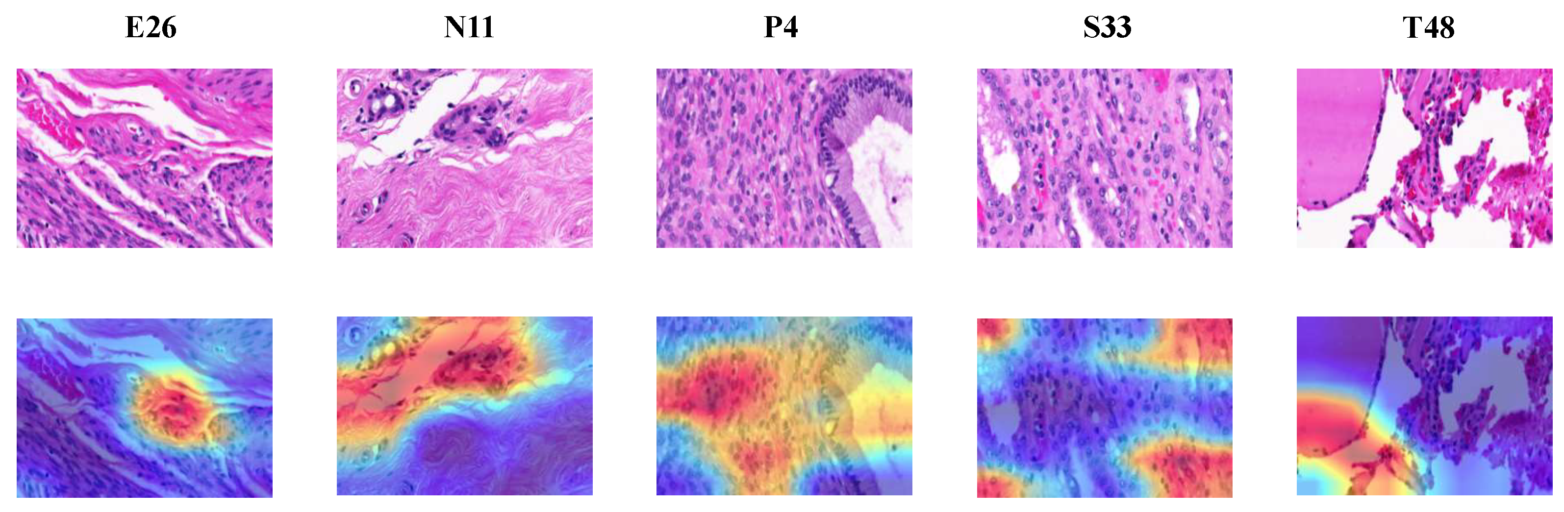
- To further test the adaptability and generalizability of the proposed methods, we interestingly validate them on KIMIA Path960, a more challenging and magnification-free histopathological image dataset. To our best knowledge, we are the first to provide such an explainable comparison based on different machine learning methods using two distinct histopathological datasets. The validation on the KIMIA Path960 dataset proves the good generalizability of the classification and visualization methods. Such visual validation on another histopathology dataset can further consolidate clinical trust in the proposed methods.
2. Related Works
3. Methods
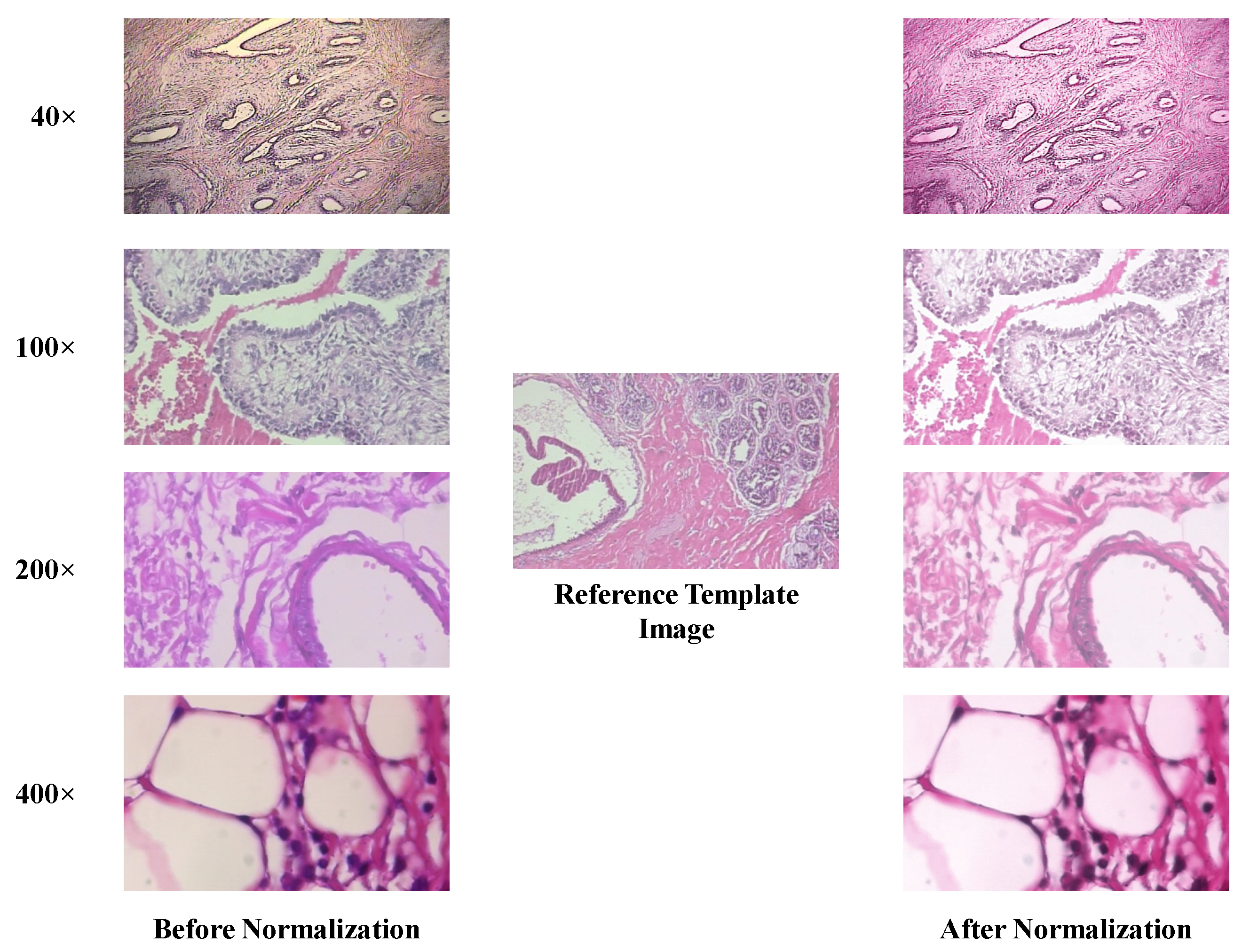
3.1. Image Pre-Processing
3.2. Conventional Machine Learning (CML) Approaches
3.2.1. Feature Extraction-Based CML Approaches
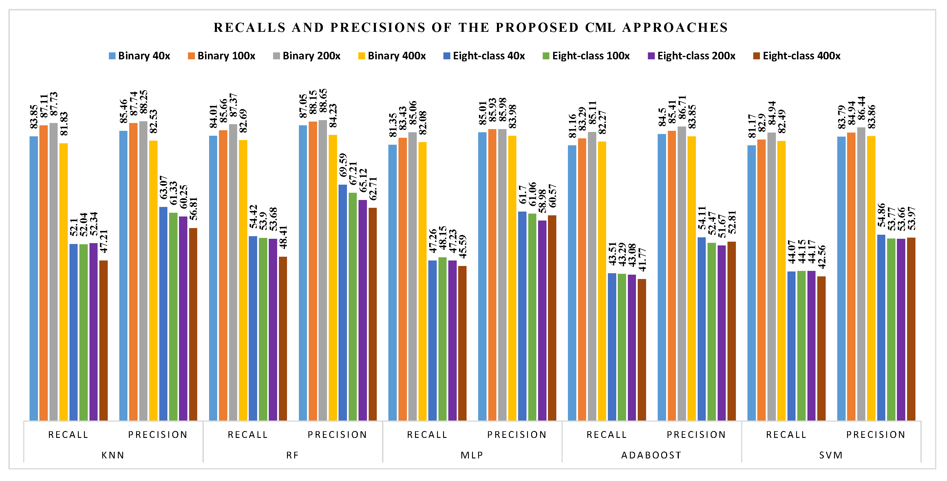
3.2.2. Classification-Based CML Approaches
3.3. Deep Learning (DL)-Based Approach
4. Performance Comparison and Visual Explanation
4.1. Setup
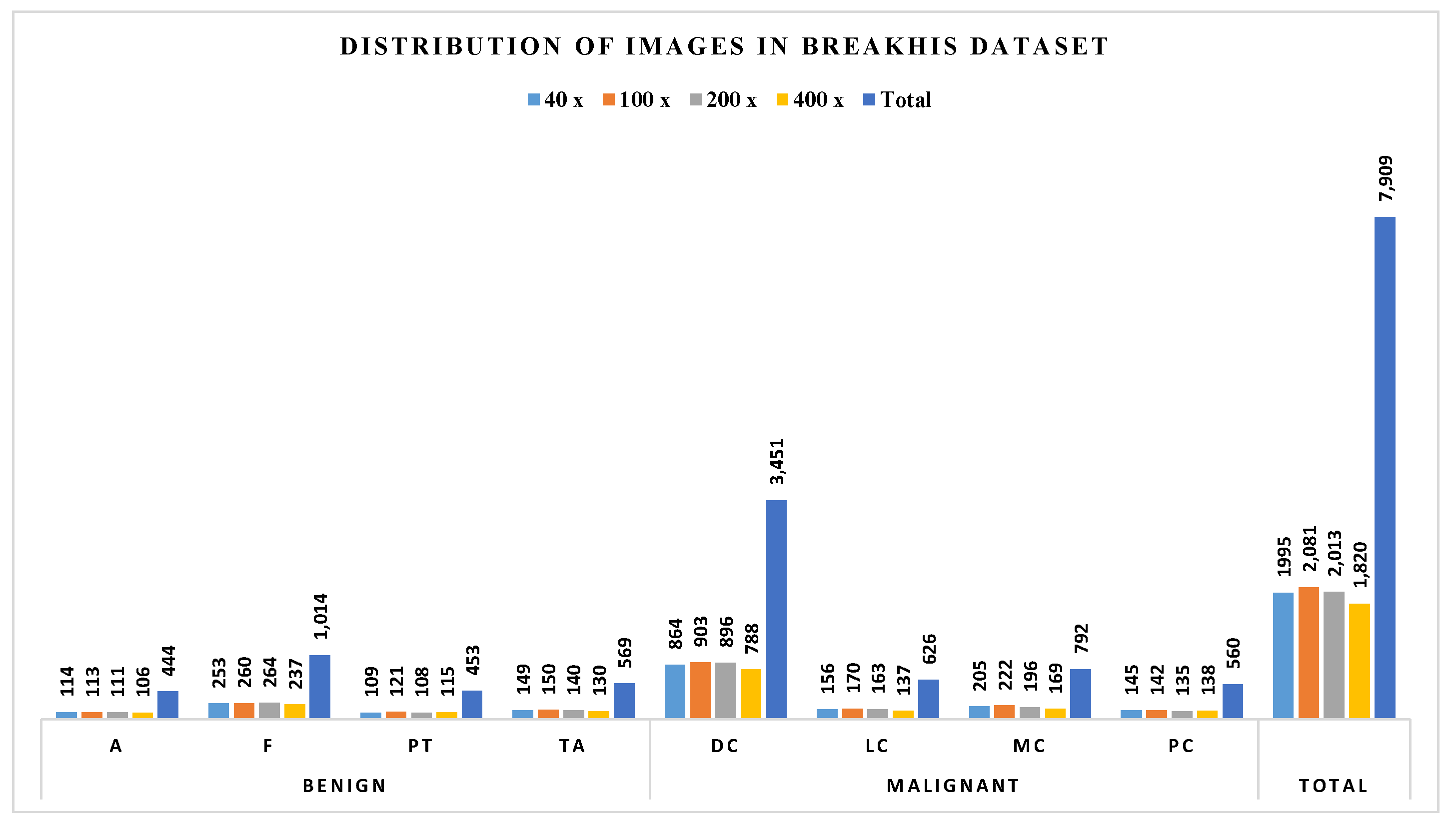
4.1.1. Datasets
4.1.2. Parameter Setting
4.1.3. Evaluation Criteria
4.2. Classification Performance Results
4.2.1. Comparison on BreaKHis Dataset
4.2.2. Validation and Comparison on the KIMIA Path960 Dataset
4.3. Visual Explanation
4.3.1. Classification Performance Explanation
4.3.2. Classification Decision Explanation of the DL Approach
4.4. Classification Comparison with Other State-of-the-Art Methods
5. Conclusions
Author Contributions
Funding
Institutional Review Board Statement
Informed Consent Statement
Data Availability Statement
Conflicts of Interest
References
- World Health Organization. Breast Cancer. 2018. Available online: http://www.who.int/cancer/prevention/diagnosis-screening/breast-cancer/en/ (accessed on 8 September 2020).
- Royal College of Pathologists. Meeting Pathology Demand. Histopathology Workforce Census. R. Coll. Pathol. 2018, 1–14. [Google Scholar]
- National Breast Cancer Foundation (NBCF). How Does Breast Cancer Start & Spread? 2021. Available online: https://nbcf.org.au/about-national-breast-cancer-foundation/about-breast-cancer/what-you-need-to-know/breast-anatomy-cancer-starts/ (accessed on 26 December 2020).
- Gurcan, M.N.; Boucheron, L.E.; Can, A.; Madabhushi, A.; Rajpoot, N.M.; Yener, B. Histopathological image analysis: A review. IEEE Rev. Biomed. Eng. 2009, 2, 147–171. [Google Scholar] [CrossRef] [Green Version]
- Zemouri, R.; Devalland, C.; Valmary-Degano, S.; Zerhouni, N. Intelligence artificielle: Quel avenir en anatomie pathologique? In Annales de Pathologie; Elsevier, 2019; Volume 39, pp. 119–129. [Google Scholar]
- Brook, A.; El-Yaniv, R.; Isler, E.; Kimmel, R.; Meir, R.; Peleg, D. Breast Cancer Diagnosis from Biopsy Images Using Generic Features and SVMs; Technical Report; Computer Science Department, Technion, 2008. [Google Scholar]
- Belsare, A.; Mushrif, M.; Pangarkar, M.; Meshram, N. Classification of breast cancer histopathology images using texture feature analysis. In Proceedings of the TENCON 2015—2015 IEEE Region 10 Conference, Macao, China, 1–4 November 2015; pp. 1–5. [Google Scholar]
- Spanhol, F.A.; Oliveira, L.S.; Petitjean, C.; Heutte, L. A dataset for breast cancer histopathological image classification. IEEE Trans. Biomed. Eng. 2015, 63, 1455–1462. [Google Scholar] [CrossRef]
- Sanchez-Morillo, D.; González, J.; García-Rojo, M.; Ortega, J. Classification of breast cancer histopathological images using KAZE features. In International Conference on Bioinformatics and Biomedical Engineering; Springer: Granada, Spain, 2018; pp. 276–286. [Google Scholar]
- Giger, M.L. Medical imaging and computers in the diagnosis of breast cancer. In Photonic Innovations and Solutions for Complex Environments and Systems (PISCES) II; International Society for Optics and Photonics: San Diego, CA, USA, 2014; Volume 9189, p. 918908. [Google Scholar]
- Zeiler, M.D.; Taylor, G.W.; Fergus, R. Adaptive deconvolutional networks for mid and high level feature learning. In Proceedings of the 2011 International Conference on Computer Vision, Barcelona, Spain, 6–13 November 2011; pp. 2018–2025. [Google Scholar]
- MIT-Technology-Review. 10 Breakthrough Technologies in 2013. 2020. Available online: https://www.technologyreview.com/10-breakthrough-technologies/2013/ (accessed on 26 December 2020).
- Zemouri, R.; Zerhouni, N.; Racoceanu, D. Deep learning in the biomedical applications: Recent and future status. Appl. Sci. 2019, 9, 1526. [Google Scholar] [CrossRef] [Green Version]
- Pan, S.J.; Yang, Q. A survey on transfer learning. IEEE Trans. Knowl. Data Eng. 2009, 22, 1345–1359. [Google Scholar] [CrossRef]
- Oquab, M.; Bottou, L.; Laptev, I.; Sivic, J. Learning and transferring mid-level image representations using convolutional neural networks. In Proceedings of the IEEE Conference on Computer Vision and Pattern Recognition, Columbus, OH, USA, 23–28 June 2014; pp. 1717–1724. [Google Scholar]
- Deng, J.; Dong, W.; Socher, R.; Li, L.J.; Li, K.; Fei-Fei, L. Imagenet: A large-scale hierarchical image database. In Proceedings of the 2009 IEEE Conference on Computer Vision and Pattern Recognition, Miami, FL, USA, 20–25 June 2009; pp. 248–255. [Google Scholar]
- Kornblith, S.; Shlens, J.; Le, Q.V. Do better imagenet models transfer better? In Proceedings of the IEEE/CVF Conference on Computer Vision and Pattern Recognition, Long Beach, CA, USA, 16–20 June 2019; pp. 2661–2671. [Google Scholar]
- Chakraborty, S.; Tomsett, R.; Raghavendra, R.; Harborne, D.; Alzantot, M.; Cerutti, F.; Srivastava, M.; Preece, A.; Julier, S.; Rao, R.M.; et al. Interpretability of deep learning models: A survey of results. In Proceedings of the 2017 IEEE Smartworld, Ubiquitous Intelligence & Computing, Advanced & Trusted Computed, Scalable Computing & Communications, Cloud & Big Data Computing, Internet of People and Smart City Innovation (smartworld/SCALCOM/UIC/ATC/CBDcom/IOP/SCI), San Francisco, CA, USA, 4–8 August 2017; pp. 1–6. [Google Scholar]
- Graziani, M.; Andrearczyk, V.; Marchand-Maillet, S.; Müller, H. Concept attribution: Explaining CNN decisions to physicians. Comput. Biol. Med. 2020, 123, 103865. [Google Scholar]
- Selvaraju, R.R.; Cogswell, M.; Das, A.; Vedantam, R.; Parikh, D.; Batra, D. Grad-cam: Visual explanations from deep networks via gradient-based localization. In Proceedings of the IEEE International Conference on Computer Vision, Venice, Italy, 22–29 October 2017; pp. 618–626. [Google Scholar]
- Boumaraf, S.; Liu, X.; Zheng, Z.; Ma, X.; Ferkous, C. A new transfer learning based approach to magnification dependent and independent classification of breast cancer in histopathological images. Biomed. Signal Process. Control 2021, 63, 102192. [Google Scholar] [CrossRef]
- Simonyan, K.; Zisserman, A. Very deep convolutional networks for large-scale image recognition. arXiv 2014, arXiv:1409.1556. [Google Scholar]
- Bardou, D.; Zhang, K.; Ahmad, S.M. Classification of breast cancer based on histology images using convolutional neural networks. IEEE Access 2018, 6, 24680–24693. [Google Scholar] [CrossRef]
- Bayramoglu, N.; Kannala, J.; Heikkilä, J. Deep learning for magnification independent breast cancer histopathology image classification. In Proceedings of the 2016 23rd International Conference on Pattern Recognition (ICPR), Cancun, Mexico, 4–8 December 2016; pp. 2440–2445. [Google Scholar]
- Spanhol, F.A.; Oliveira, L.S.; Petitjean, C.; Heutte, L. Breast cancer histopathological image classification using convolutional neural networks. In Proceedings of the 2016 International Joint Conference on Neural Networks (IJCNN), Vancouver, BC, Canada, 24–29 July 2016; pp. 2560–2567. [Google Scholar]
- Krizhevsky, A.; Sutskever, I.; Hinton, G.E. Imagenet classification with deep convolutional neural networks. Adv. Neural Inf. Process. Syst. 2012, 25, 1097–1105. [Google Scholar] [CrossRef]
- Nejad, E.M.; Affendey, L.S.; Latip, R.B.; Bin Ishak, I. Classification of histopathology images of breast into benign and malignant using a single-layer convolutional neural network. In Proceedings of the International Conference on Imaging, Signal Processing and Communication, Penang, Malaysia, 26–28 July 2017; pp. 50–53. [Google Scholar]
- Li, Q.; Li, W. Using Deep Learning for Breast Cancer Diagnosis; The Chinese University of Hong Kong: Hong Kong, China, 2017. [Google Scholar]
- Nahid, A.A.; Mikaelian, A.; Kong, Y. Histopathological breast-image classification with restricted Boltzmann machine along with backpropagation. Biomed. Res. 2018, 29, 2068–2077. [Google Scholar] [CrossRef] [Green Version]
- Nahid, A.A.; Mehrabi, M.A.; Kong, Y. Histopathological breast cancer image classification by deep neural network techniques guided by local clustering. BioMed Res. Int. 2018, 2018, 2362108. [Google Scholar] [CrossRef]
- Nahid, A.A.; Kong, Y. Histopathological breast-image classification using local and frequency domains by convolutional neural network. Information 2018, 9, 19. [Google Scholar] [CrossRef] [Green Version]
- Baltres, A.; Al Masry, Z.; Zemouri, R.; Valmary-Degano, S.; Arnould, L.; Zerhouni, N.; Devalland, C. Prediction of Oncotype DX recurrence score using deep multi-layer perceptrons in estrogen receptor-positive, HER2-negative breast cancer. Breast Cancer 2020, 27, 1007–1016. [Google Scholar] [CrossRef]
- Zemouri, R.; Omri, N.; Devalland, C.; Arnould, L.; Morello, B.; Zerhouni, N.; Fnaiech, F. Breast cancer diagnosis based on joint variable selection and constructive deep neural network. In Proceedings of the 2018 IEEE 4th Middle East Conference on Biomedical Engineering (MECBME), Tunis, Tunisia, 28–30 March 2018; pp. 159–164. [Google Scholar]
- Zemouri, R.; Omri, N.; Morello, B.; Devalland, C.; Arnould, L.; Zerhouni, N.; Fnaiech, F. Constructive deep neural network for breast cancer diagnosis. IFAC-PapersOnLine 2018, 51, 98–103. [Google Scholar] [CrossRef]
- Thuy, M.B.H.; Hoang, V.T. Fusing of deep learning, transfer learning and gan for breast cancer histopathological image classification. In International Conference on Computer Science, Applied Mathematics and Applications; Springer: Hanoi, Vietnam, 2019; pp. 255–266. [Google Scholar]
- Song, Y.; Zou, J.J.; Chang, H.; Cai, W. Adapting fisher vectors for histopathology image classification. In Proceedings of the 2017 IEEE 14th International Symposium on Biomedical Imaging (ISBI 2017), Melbourne, VIC, Australia, 18–21 April 2017; pp. 600–603. [Google Scholar]
- Zhi, W.; Yueng, H.W.F.; Chen, Z.; Zandavi, S.M.; Lu, Z.; Chung, Y.Y. Using transfer learning with convolutional neural networks to diagnose breast cancer from histopathological images. In International Conference on Neural Information Processing; Springer: Guangzhou, China, 2017; pp. 669–676. [Google Scholar]
- de Matos, J.; Britto, A.d.S.; Oliveira, L.E.; Koerich, A.L. Double transfer learning for breast cancer histopathologic image classification. In Proceedings of the 2019 International Joint Conference on Neural Networks (IJCNN), Budapest, Hungary, 14–19 July 2019; pp. 1–8. [Google Scholar]
- Mehra, R. Breast cancer histology images classification: Training from scratch or transfer learning? ICT Express 2018, 4, 247–254. [Google Scholar]
- Saxena, S.; Shukla, S.; Gyanchandani, M. Pre-trained convolutional neural networks as feature extractors for diagnosis of breast cancer using histopathology. Int. J. Imaging Syst. Technol. 2020, 30, 577–591. [Google Scholar] [CrossRef]
- Gour, M.; Jain, S.; Sunil Kumar, T. Residual learning based CNN for breast cancer histopathological image classification. Int. J. Imaging Syst. Technol. 2020, 30, 621–635. [Google Scholar] [CrossRef]
- He, K.; Zhang, X.; Ren, S.; Sun, J. Deep residual learning for image recognition. In Proceedings of the IEEE Conference on Computer Vision and Pattern Recognition, Las Vegas, NV, USA, 27–30 June 2016; pp. 770–778. [Google Scholar]
- Holzinger, A.; Biemann, C.; Pattichis, C.S.; Kell, D.B. What do we need to build explainable AI systems for the medical domain? arXiv 2017, arXiv:1712.09923. [Google Scholar]
- Chen, C.; Li, O.; Tao, C.; Barnett, A.J.; Su, J.; Rudin, C. This looks like that: Deep learning for interpretable image recognition. arXiv 2018, arXiv:1806.10574. [Google Scholar]
- Samek, W.; Wiegand, T.; Müller, K.R. Explainable artificial intelligence: Understanding, visualizing and interpreting deep learning models. arXiv 2017, arXiv:1708.08296. [Google Scholar]
- Tellez, D.; Litjens, G.; van der Laak, J.; Ciompi, F. Neural image compression for gigapixel histopathology image analysis. IEEE Trans. Pattern Anal. Mach. Intell. 2019, 43, 567–578. [Google Scholar] [CrossRef] [PubMed] [Green Version]
- Weng, W.H.; Cai, Y.; Lin, A.; Tan, F.; Chen, P.H.C. Multimodal multitask representation learning for pathology biobank metadata prediction. arXiv 2019, arXiv:1909.07846. [Google Scholar]
- Zhang, Z.; Chen, P.; McGough, M.; Xing, F.; Wang, C.; Bui, M.; Xie, Y.; Sapkota, M.; Cui, L.; Dhillon, J.; et al. Pathologist-level interpretable whole-slide cancer diagnosis with deep learning. Nat. Mach. Intell. 2019, 1, 236–245. [Google Scholar] [CrossRef]
- Huang, Y.; Chung, A.C. Evidence localization for pathology images using weakly supervised learning. In International Conference on Medical Image Computing and Computer-Assisted Intervention; Springer: Shenzhen, China, 2019; pp. 613–621. [Google Scholar]
- BenTaieb, A.; Hamarneh, G. Predicting cancer with a recurrent visual attention model for histopathology images. In International Conference on Medical Image Computing and Computer-Assisted Intervention; Springer: Granada, Spain, 2018; pp. 129–137. [Google Scholar]
- Vahadane, A.; Peng, T.; Sethi, A.; Albarqouni, S.; Wang, L.; Baust, M.; Steiger, K.; Schlitter, A.M.; Esposito, I.; Navab, N. Structure-preserving color normalization and sparse stain separation for histological images. IEEE Trans. Med Imaging 2016, 35, 1962–1971. [Google Scholar] [CrossRef] [PubMed]
- Teague, M.R. Image analysis via the general theory of moments. JOSA 1980, 70, 920–930. [Google Scholar] [CrossRef]
- Khotanzad, A.; Hong, Y.H. Invariant image recognition by Zernike moments. IEEE Trans. Pattern Anal. Mach. Intell. 1990, 12, 489–497. [Google Scholar] [CrossRef] [Green Version]
- Wang, W.; Mottershead, J.E.; Mares, C. Mode-shape recognition and finite element model updating using the Zernike moment descriptor. Mech. Syst. Signal Process. 2009, 23, 2088–2112. [Google Scholar] [CrossRef]
- Hosny, K.M. Fast computation of accurate Zernike moments. J. Real-Time Image Process. 2008, 3, 97–107. [Google Scholar] [CrossRef]
- Tahmasbi, A.; Saki, F.; Shokouhi, S.B. Classification of benign and malignant masses based on Zernike moments. Comput. Biol. Med. 2011, 41, 726–735. [Google Scholar] [CrossRef]
- Haralick, R.M.; Shanmugam, K.; Dinstein, I.H. Textural features for image classification. IEEE Trans. Syst. Man. Cybern. 1973, 610–621. [Google Scholar] [CrossRef] [Green Version]
- Boumaraf, S.; Liu, X.; Ferkous, C.; Ma, X. A new computer-aided diagnosis system with modified genetic feature selection for bi-RADS classification of breast masses in mammograms. BioMed Res. Int. 2020, 7695207. [Google Scholar] [CrossRef]
- Ferkous, C.; Merouani, H.F. Mammographic mass classification according to Bi-RADS lexicon. IET Computer Vision 2016, 11, 189–198. [Google Scholar]
- Swati, Z.N.K.; Zhao, Q.; Kabir, M.; Ali, F.; Ali, Z.; Ahmed, S.; Lu, J. Brain tumor classification for MR images using transfer learning and fine-tuning. Comput. Med Imaging Graph. 2019, 75, 34–46. [Google Scholar] [CrossRef] [PubMed]
- Kumar, M.D.; Babaie, M.; Zhu, S.; Kalra, S.; Tizhoosh, H.R. A comparative study of CNN, BoVW and LBP for classification of histopathological images. In Proceedings of the 2017 IEEE Symposium Series on Computational Intelligence (SSCI), Honolulu, HI, USA, 27 November–1 December 2017; pp. 1–7. [Google Scholar]
- Kingma, D.P.; Ba, J. Adam: A method for stochastic optimization. arXiv 2014, arXiv:1412.6980. [Google Scholar]
- Jolliffe, I.T.; Cadima, J. Principal component analysis: A review and recent developments. Philos. Trans. R. Soc. A Math. Phys. Eng. Sci. 2016, 374, 20150202. [Google Scholar] [CrossRef]
- Schölkopf, B.; Smola, A.; Müller, K.R. Nonlinear component analysis as a kernel eigenvalue problem. Neural Comput. 1998, 10, 1299–1319. [Google Scholar] [CrossRef] [Green Version]
- Dif, N.; Elberrichi, Z. A New Intra Fine-Tuning Method Between Histopathological Datasets in Deep Learning. Int. J. Serv. Sci. Manag. Eng. Technol. (IJSSMET) 2020, 11, 16–40. [Google Scholar] [CrossRef]


| Classification Scheme | Magnification Factor | KNN | RF | MLP | AdaBoost | SVM |
|---|---|---|---|---|---|---|
| Binary | 40× | 87.04 | 87.69 | 85.85 | 85.67 | 85.26 |
| 100× | 89.32 | 88.94 | 87.18 | 86.86 | 86.51 | |
| 200× | 89.75 | 89.82 | 88.26 | 88.16 | 87.97 | |
| 400× | 84.53 | 85.65 | 85.31 | 85.31 | 85.38 | |
| Eight-class | 40× | 65.28 | 68.44 | 64.41 | 56.98 | 58.16 |
| 100× | 65.59 | 68.17 | 65.08 | 56.90 | 58.37 | |
| 200× | 67.02 | 69.69 | 66.42 | 59.02 | 60.44 | |
| 400× | 60.40 | 63.55 | 62.28 | 55.10 | 56.46 |
| Classification Scheme | Magnification Factor | Accuracy Based on Block-Wise Fine-Tuning Strategy | |||||
|---|---|---|---|---|---|---|---|
| B6 | B6-B5 | B6-B4 | B6-B3 | B6-B2 | B6-B1 | ||
| Binary | 40× | 53.23 | 88.27 | 94.56 | 98.13 | 97.96 | 97.45 |
| 100× | 74.27 | 88.76 | 94.79 | 94.95 | 97.39 | 96.09 | |
| 200× | 73.74 | 85.52 | 93.10 | 94.95 | 96.63 | 94.95 | |
| 400× | 68.03 | 83.27 | 89.03 | 94.05 | 92.38 | 91.64 | |
| Eight-class | 40× | 31.80 | 74.83 | 80.95 | 88.95 | 88.27 | 85.88 |
| 100× | 44.79 | 65.96 | 79.15 | 79.80 | 83.22 | 83.71 | |
| 200× | 49.49 | 60.44 | 76.94 | 79.63 | 80.64 | 79.12 | |
| 400× | 47.03 | 56.69 | 67.29 | 76.77 | 72.49 | 76.39 | |
| Classification Algorithm | Accuracy | Recall | Precision |
|---|---|---|---|
| KNN | 88.54 | 87.25 | 88.49 |
| RF | 93.45 | 92.89 | 93.47 |
| MLP | 83.19 | 82.64 | 80.50 |
| AdaBoost | 68.34 | 68.02 | 64.77 |
| SVM | 74.37 | 74.19 | 71.62 |
| Block-Wise Fine-Tuning Strategy | Accuracy | Recall | Precision |
|---|---|---|---|
| B6 | 68.06 | 68.00 | 74.51 |
| B6-B5 | 89.58 | 90.13 | 91.17 |
| B6-B4 | 96.53 | 96.49 | 96.37 |
| B6-B3 | 98.26 | 97.96 | 98.12 |
| B6-B2 | 98.26 | 98.31 | 98.48 |
| B6-B1 | 97.92 | 98.02 | 98.23 |
| Reference | Method Used | Accuracy Performance (%) | |||
|---|---|---|---|---|---|
| 40× | 100× | 200× | 400× | ||
| Spanhol et al [8]. | Completed LBP features with SVM classifier. | 77.40 | 76.40 | 70.20 | 72.80 |
| Sanchez-Morillo et al [9]. | KAZE features combined with Bag-of-Features with binary SVM classifier. | 85.90 | 80.40 | 78.10 | 71.30 |
| Bayramoglu et al [24]. | A deep CNN model which is variant of AlexNet | 89.60 | 85.00 | 84.00 | 80.80 |
| Spanhol et al [25]. | Single task architecture based on a deep CNN model with a softmax layer on top. | 83.00 | 83.10 | 84.60 | 82.10 |
| This work | Zernike moments, Haralick, and color histogram features all fused and classified with five standalone classifiers. | 87.69 | 89.32 | 89.82 | 85.65 |
| Block-wise fine-tuned VGG-19 model with softmax classifier on top. | 98.13 | 97.39 | 96.63 | 94.05 | |
| Reference | Method Used | Accuracy Performance (%) | |||
|---|---|---|---|---|---|
| 40× | 100× | 200× | 400× | ||
| Bardou et al [23]. | SURF features encoded with bag of words (BoW) and classified with SVM. | 49.65 | 47.00 | 38.84 | 29.50 |
| SURF features encoded with locality constrained linear coding and classified with SVM. | 55.80 | 54.24 | 40.83 | 37.20 | |
| Deep CNN features (trained from scratch) with KNN classifier on top. | 70.48 | 68.00 | 70.08 | 66.38 | |
| Deep CNN features (trained from scratch) with Linear SVM classifier on top. | 72.35 | 67.68 | 66.45 | 64.95 | |
| This work | Zernike moments, Haralick, and color histogram features all fused and classified with five standalone classifiers. | 87.69 | 89.32 | 89.82 | 85.65 |
| Block-wise fine-tuned VGG-19 model with softmax classifier on top. | 98.13 | 97.39 | 96.63 | 94.05 | |
| Reference | Method Used | Accuracy Performance (%) |
|---|---|---|
| Kumar et al [61]. | LBP features with two types of distance measures (Chi-squared and Euclidean distance). | 90.62 |
| Bag of visual words (BoVW) features with histogram intersection kernel SVM classifier. | 96.50 | |
| Deep features based on pre-trained AlexNet and VGG-16 models. | 94.72 | |
| Dif and Elberrichi [65]. | Transfer learning based on Inception-v3 CNN architecture, six histopathological source datasets, and four target datasets. | 98.18 |
| This work | Zernike moments, Haralick, and color histogram features all fused and classified with five standalone classifiers. | 93.45 |
| Block-wise fine-tuned VGG-19 model with softmax classifier on top. | 98.26 |
Publisher’s Note: MDPI stays neutral with regard to jurisdictional claims in published maps and institutional affiliations. |
© 2021 by the authors. Licensee MDPI, Basel, Switzerland. This article is an open access article distributed under the terms and conditions of the Creative Commons Attribution (CC BY) license (http://creativecommons.org/licenses/by/4.0/).
Share and Cite
Boumaraf, S.; Liu, X.; Wan, Y.; Zheng, Z.; Ferkous, C.; Ma, X.; Li, Z.; Bardou, D. Conventional Machine Learning versus Deep Learning for Magnification Dependent Histopathological Breast Cancer Image Classification: A Comparative Study with Visual Explanation. Diagnostics 2021, 11, 528. https://doi.org/10.3390/diagnostics11030528
Boumaraf S, Liu X, Wan Y, Zheng Z, Ferkous C, Ma X, Li Z, Bardou D. Conventional Machine Learning versus Deep Learning for Magnification Dependent Histopathological Breast Cancer Image Classification: A Comparative Study with Visual Explanation. Diagnostics. 2021; 11(3):528. https://doi.org/10.3390/diagnostics11030528
Chicago/Turabian StyleBoumaraf, Said, Xiabi Liu, Yuchai Wan, Zhongshu Zheng, Chokri Ferkous, Xiaohong Ma, Zhuo Li, and Dalal Bardou. 2021. "Conventional Machine Learning versus Deep Learning for Magnification Dependent Histopathological Breast Cancer Image Classification: A Comparative Study with Visual Explanation" Diagnostics 11, no. 3: 528. https://doi.org/10.3390/diagnostics11030528