1. Introduction
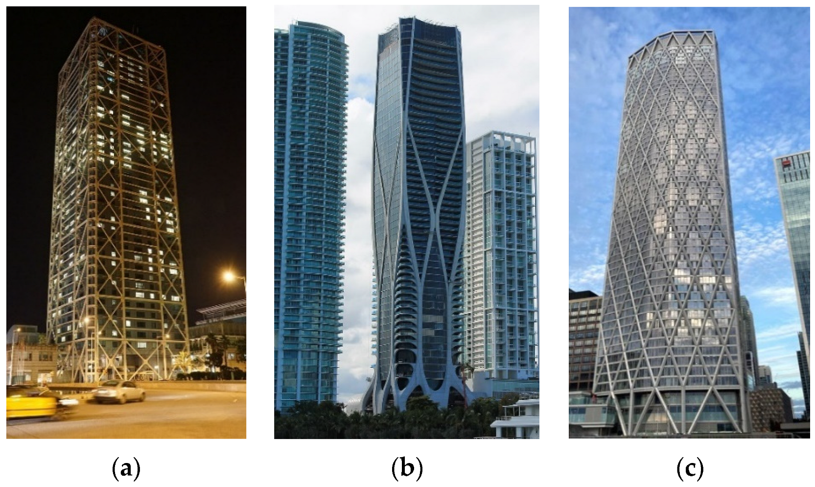
Modern high-rise buildings are often inspired by nature, and they significantly change large cities all over the world. Their atypical shape is the result of the amazing imagination of architects. Among those who were not afraid to experiment were Zaha Hadid, Roger Strik Harbour + Partners, Bruce John Graham, Richard Rogers, Norman Foster, and Horden Cherry Lee. These structures are so extraordinary (
Figure 1), that most people have a clear opinion on whether they are beautiful works or ugly structures.
Many modern structures are also interesting for tourists and for photographers. Therefore, they make the cities more famous. On the other hand, their design and the construction are financially demanding and time consuming for investors. Expensive and difficult technologies are required for their construction. Civil engineers have to determine appropriate input parameters for the design of structures, e.g., soil parameters, applied loads, wind load, and temperature load. Most of the buildings have an atypical shape, as seen in
Figure 2. Therefore, wind tunnel testing (WT) and/or computational fluid dynamics (CFD) are necessary for the determination of wind effects on the structure. The CFD is a good tool, but there are many possibilities for modelling and methods (turbulence models) for the solution. The important question is as follows: which is the exact method and which setting is correct for the solution of a structure like this? Wind tunnel testing is expensive, time-consuming, and there are some limitations with respect to the very small scale of the model. Therefore, the combination of both mentioned methods is the best solution.
High-rise buildings are more affected by wind load than lower buildings, due to their large external areas. They are exposed to high wind velocities, and they are not protected by other, higher buildings. Wind gusts during strong windstorms can be very dangerous because they can cause large vibrations [
7]. Another problem is wind-driven rain, which is dangerous for façade elements [
8]. Additionally, the places with large negative pressures are not suitable for the placement of passive ventilation devices because they work only in limited pressure range.
There are some other influences which have to be considered in the design and assessment of the structure (e.g., vibrations due to devices placed inside the structure, shrinkage and creep of the concrete, and temperature effects). The ratio of the total height of the structure to the dimensions of ground plan is large. Hence, this type of structure is similar to a cantilever beam (the bottom part is fixed to the ground and the upper part is a free end). There are many horizontal slabs which make the building stiffer and help to resist a horizontally applied load (the wind load). The most commonly used materials are reinforced concrete, steel, or their combination.
The Investigation of the Wind Effects on Tall/High-Rise Buildings and New Solutions
This paper deals with wind analysis, specifically the determination of the mean external wind pressure coefficients. There are many interesting papers dealing with the investigation of wind pressure distribution and other wind effects occurring on tall or high-rise buildings. One of the many important parts of each building is its façade. The problem of tall slender structures is their vulnerability to wind-induced vibrations. A good solution can be the use of smart façades, which are adaptive and useful for architectural and energy-saving applications. More information can be found in [
9]. In [
10], the same authors compared the wind-induced effects on a tall building with rectangular and elliptical double-skin façades. They used the optimization approach in order to minimalize the wind load applied on the structure. The evaluation was carried out using the calculation of drag coefficient.
A study dealing with the modification of the façade of a tall building by the ribs in order to reduce the wind effects is mentioned in [
11]. This study was supported by the results from wind tunnel tests obtained by the particle image velocimetry (PIV) technique. In the continuous study [
12], the authors observed that the windward face ribs and downstream sidewall ribs can affect the behavior of the separated shear layer. The upstream ribs of side wall and leeward side ribs did not have a significant effect on the flow field and aerodynamic force. However, it is better to design ribs on all sides of the building (from a practical point of view). They observed that the distance between the ribs is a very important parameter because the free space between the ribs has an influence on the modification of the flow structure and the wind load applied on the structure.
The largest value of local peak pressures on the cladding of tall building and unfavorable wind directions are determined by wind tunnel tests in [
13]. Additionally, in this case, the decrease in the local wind pressures was made by the modification of the façade of the structure and not by the changing of the total shape of the structure (contrary to our solution, where the local pressures were decreased by changing the total shape of the structure). In the next paper [
14], the same authors continued in the study. They calculated the aerodynamic forces of the high-rise building (including the mean and fluctuating base moment, layer force, power spectral densities, correction, and coherence).
Wind pressure distribution can also be changed by using the balconies on the façade of a tall cuboid building [
15]. In this analysis, two methods were used, namely CFD simulation and wind tunnel tests. Mainly, our analysis focused on the differences in the modelling and in the results obtained by two different turbulence modes—LES (large-eddy simulation) and RANS (Reynolds-averaged Navier–Stokes). Only three wind directions, namely 0°, 90°, and 180°, were considered. Another comprehensive study dealing with the influence of wind flow on different types of balconies (various positions of the balconies on the façade of the structure, density of the balconies, various depths, influence of balcony parapet walls, balconies with or without the partition walls, etc.) is presented in [
16]. These balconies were designed as continuous on two opposite sides of the building. Other two sides were smooth. Two wind directions were investigated, namely 0° and 180°. One of the important results is that the presence of the balconies on the façade of the structure can cause the increase in the mean wind pressure coefficient. The pressure coefficients were significantly smaller only in the case of five partition walls. The authors used LES with very fine mesh in combination with the wind tunnel data.
Wind pressure distribution can be modified by changing the shape of the structure. Therefore, it can be useful to know the influence of geometrical shape on the wind flow and vortex separation. This is the main topic of [
17], where the wind effects on the building are investigated in detail. Torsional effects and resultant wind forces were calculated for five different geometrical shapes of the buildings (square, triangular, rectangular, circular, and elliptic). Triangular, elliptic, and rectangular shaped buildings were identified as being especially sensitive to torsional wind effects. For the evaluation of the wind pressure distribution on the structure, the very important parameter is the Reynolds number. If the Reynolds number is not satisfied, the
cpe are influenced. More information and the importance of Reynolds number, as proved by several researchers, can be found in [
18,
19,
20].
The interference wind effects between two tall cuboid buildings with smooth surfaces in a staggered arrangement was investigated in [
21]. Two methods, CFD simulation using the LES, and the PIV technique in a wind tunnel, were used. Both buildings had the same dimensions—the height was 180 m, and the square ground-plan had edges 30 m in length. In this case, the height of the model was divided into six measured levels. In each level, 20 measuring taps were installed. In this study, the advanced methods (time-averaged mean and fluctuating streamwise and transverse velocity distribution, the large-scale coherent pattern, and in-phase synchronization of the vortex shedding from both buildings) were used. Here,
cpe were not denominated.
2. Description of the Investigated Building
The investigated structure was a slender and tall architecturally attractive multi-purpose building. The original shape was cuboid, but this was significantly changed by the architect. In the bottom part of the building, the ground plan had the shape of a square with dimensions of 30 m × 30 m. On the top of the building, the ground plan was polygon with the following dimensions: 32.4 m, 17.8, 17.8 m, and 32.4 m, as shown in
Figure 3. The total height of this 44-story high-rise building was 162 m above the ground. Another four stories were designed in the underground part of the building.
The thickness of horizontal composite slabs made of C30/37 concrete and S 235 steel was 200 mm. The vertical structural system was made of the combination of a stiffened reinforced concrete core (the thickness of the walls was 300 mm, C40/50) and a steel exoskeleton structure placed on the perimeter of the building. The cladding of the structure was made of the aluminum frame with triple insulating glass, with a thickness of 200 mm and a density equal to 300 kg/m3.
The reinforced concrete foundation plate with the thickness of 3 m was combined with reinforced concrete piles (Ø 1.2 m). The subsoil was considered as stiff without the influence of the ground water on the underground walls of the structure.
The building was divided into the following parts according to its purpose: flats, apartments, hotel, offices, and underground parking. The construction height of a typical floor was 3.6 m (the first floor and the second floor were 7.4 m high, while the last floor was 3.0 m high). The building was located in Bratislava (the capital city of Slovakia) in a uniformly built-up area. The design of the structure and all its structural elements (the foundations, horizontal slabs, the walls, and all columns) were carried out according to requirements defined in [
22,
23,
24,
25,
26]. The commercial program Scia Engineer, which uses the finite element method (FEM) for the solution of created models, was chosen for static and dynamic analysis of the structure.
Static and Dynamic Analysis of the Investigated Building
The main topic of this paper is the determination of wind effects on the façade of the investigated building. Therefore, only short information about static and dynamic analysis is mentioned here. Two requirements of the architect were obligatory. The first was that the architectural design of the building was mandatory and could not be changed. The second was that interior spaces had to be designed as open-air spaces with minimum vertical structural elements, such as walls and the columns, inside. Therefore, the design and assessment of the structural system was very difficult.
The analysis was divided into two parts. As first, the analysis was focused on the design and placement of vertical structural elements. Horizontal composite slabs and vertical stiffening walls of the reinforced concrete core were added by the main stiffening elements of an exoskeleton system and by steel columns in the corners of ground plan (Ø 914 mm/
t = 14.2 mm). Then, other vertical columns (Ø 457 mm/
t = 12.5 mm) with axial distances equal to 5 m were placed on the perimeter of the ground plan. After that, the columns were changed from vertical to diagonal. For all investigated models of the structure, static and dynamic analysis was carried out, and a serviceability limit state was advised. In the case of static analysis, the maximum vertical displacements of the top slab due to wind were compared with the limit value defined in the standards, namely
umax = H/2000 (where
H was the total height of the structure). In the case of dynamic analysis, the limit value defined in the standards was
umax = H/500. Additionally, eigenfrequencies and eigenmodes were calculated. More information can be found in [
27].
The second analysis was used for the optimization of the parameters of the exoskeleton structure (the diameter and the thickness of steel tubes). The basic criterium was the same as it was in the first analysis (the comparison of the maximum horizontal displacement with the limit value defined in the standards). More information can be found in [
28,
29].
3. Boundary Layer Wind Tunnel, Methodology of the Tests and Reduced-Scale Model
In the aforementioned static analysis, wind load was applied on the structure by using a 3D wind generator included in the program Scia Engineer. The model of the same structure was investigated in a boundary layer wind tunnel because of the better estimation of the mean external pressure coefficients.
In our case, this task was solved as stationary (without the consideration of dynamic wind effects—because of missing appropriate measuring devices). The model was static (the stiffness of the model was larger in comparison to the real structure), but the recommended Reynolds number was satisfied. Mean external pressure coefficients were estimated.
Reduced-scale models of the cuboid and the atypical structure in 1:300 are shown in
Figure 4 and
Figure 5. For this analysis, only the model of atypical structure was tested in a wind tunnel (the results are discussed in this paper). Both models were important for the follow-up analysis, namely the investigation of the wind flow around/on the building complex. The distance between both buildings was changed in a given range and the extreme values of mean external pressure coefficients, drag coefficients, and lift coefficients were determined for different wind directions. Additionally, the wind effects on pedestrians walking around the buildings were investigated.
The sampling frequency was 500 Hz, and the measurement time was 60 s. Mean external pressure coefficients were calculated from two repeated measurements. Equation (1) is as follows:
where
cpe is the mean external pressure coefficient [-],
PWT is the average value of external wind pressure measured in given point [Pa], and
Pref is the reference pressure [Pa]. Equation (2) is as follows:
where
ρ is air density [kg/m
3] defined as a function (Equation (3)) of he measured air temperature
T in [°] and the atmospheric pressure
BP in [Pa], and
vref is the reference wind velocity measured on the top of the building without the model.
The model of the atypical structure was created through a combination of 3D printing and plexiglass with a thickness of 4 mm, as seen in
Figure 4. The model of the cuboid was made of the plexiglass with the same thickness.
The measuring taps were made of very short brass tubes fixed by special methacrylate glue and vinyl tubes connected to pneumatic connector 19F460 (Scanivalve). Wind pressures were measured using 2 DSA 3217/16 16-channel pressure scanners (the measured range up to 2.5 kPa, and the device is produced by Scanivalve). A hot-wire anemometer miniCTA 54T42 (Dantec Dynamics) was used for the measurement of reference wind velocity in the height of the top of the building. The sampling frequency was 3000 Hz, and the number of samples was 300,000. A Prandtl tube located on the wall of the wind tunnel (inside the wind tunnel, not affected by wall effects) was used as a reference probe during the tests. Uniformity of wind pressures along the whole wind tunnel was controlled by 16 differential pressure sensors located under the adjustable ceiling of the wind tunnel. All parameters, e.g., the air temperature, atmospheric pressure, wind pressures, and wind velocities, were recorded by the self-developed program created in the commercial software LabView (National Instruments). Detailed information about the BLWT in Bratislava, which belongs to Slovak University of Technology in Bratislava, the dimensions of the tunnel, its utilization, measuring devices, and the accuracy of obtained results from previous research can be found in [
30,
31,
32,
33].
The dimensions of the reduced-scale models in [mm] with marked measuring taps are shown in
Figure 5. In the case of the cuboid, the perimeter was constant at all levels. In the case of an atypical structure, the perimeter at measured levels was different (level A—338 mm, level B—356 mm, level C—368 mm, and level D—388 mm).
Air temperature during the test (
Figure 6a) was 15.8 °C, and atmospheric pressure was 101,140 Pa. With regard to these conditions, the measured reference wind velocities were 8.858 m/s and 10.951 m/s (the results in this paper are presented only for this reference velocity). A terrain category between III and IV (according to [
25]) with a roughness length
z0 equal to 0.7 was considered. This was modelled using a wooden barrier with a height of 150 mm, and the plastic film FASTREADE 20. All investigated wind directions are shown in
Figure 6b.
4. CFD Simulation—Turbulence Model, Boundary Conditions, the Validation
It was confirmed by the results of previous research dealing with the simulation of wind flow around structures or in large urban areas [
34,
35,
36,
37] that the choice of the appropriate turbulence model is crucial. Different engineering problems of wind flow require the use of different turbulence models or the solutions [
38,
39,
40,
41]. Hence, an engineer has to have either theoretical knowledge and experience from previous research, or he/she should use several types of turbulence models, compare their results, and then select the best one. When considering different turbulence models, smaller or larger discrepancies in the results can be observed. For the validation of the performance of turbulence models, the method of three metrics—fractional bias (
FB), correlation coefficient (
R) and fraction of data within a factor of 1.3 (
FAC 1.3)—can be employed [
42,
43].
The following turbulence models are among the most used: the standard k-ε model (RANS), the realizable k-ε model (RANS), the renormalization group k-ε model (RANS), the standard k-ω model (RANS), the shear stress transport k-ω model (RANS), and large-eddy simulation (LES). The last-mentioned method is more sophisticated, as it requires the setting of very fine computational grid and very small time steps. Hence, a more powerful computer is essential, and the solution by this method is significantly more time-consuming. More information can be found in [
44,
45,
46,
47,
48,
49].
4.1. Computational Domain, Boundary Conditions, and Computational Grid
The results obtained by CFD simulation can be significantly affected by its settings, and also by the modelling of the structure. Geometrical simplifications, e.g., the material of the façade, small details on the structure, etc., are allowed. However, they should be considered carefully. The computational domain should be large and the computational grid should be sufficiently small. The very important issues are as follows: the selection and the application of boundary conditions, and the determination of the sand-grain roughness height.
When the CFD simulation is compared with data from wind tunnel tests, the computational domain can be modelled in two ways. The first way is when the computational domain has the same dimensions as an operating space in a wind tunnel. The investigated structure is modelled in a reduced-scale. The boundary conditions can be considered by the real material of the wind tunnel (real-material case). The second way is when a computational model is created as the real structure. The total dimensions of the computational domain are also multiplied by the geometrical scale of the model used in the wind tunnel. Applied boundary conditions can be considered by appropriate function (in a standard case).
A realizable k-ε turbulence model was selected with respect to the authors’ experiences obtained from previous studies. This type of turbulence model reached the best coincidence with data from wind tunnel tests in similar analyzed engineering problems, e.g., [
50]. The reduced-scale model was modelled. The commercial software Ansys Fluent using the finite volume method was selected for the modelling and for the analysis.
The surface roughness height was applied on the boundaries of the computational domain by using aerodynamic roughness length z0 (for a uniformly built-up area). It is defined as the height above the ground where the wind velocity drops to zero. Total dimensions of computation domain were 1.6 m × 2.6 m × 7 m, H × W × L, respectively, because of the recommendation that the ratio of the size of investigated building to the size of computational domain be less than 3%. By satisfying this recommendation, the results obtained by CFD simulation should not be affected by the boundaries of the domain. The width and height of the computational domain was equal to the dimensions of the cross-section of the rear operating space in the wind tunnel.
The computational domain was divided into three parts (
Figure 7a). The model was situated in the main part where the computational grid was very fine. The other two parts had a larger computational grid. The urban terrain was considered at the bottom of the computational domain.
The computational grid was created by using hexacore elements [
51] of various sizes (2.5 mm at the surface of the model, up to 100 mm in other parts). Approximately 600,000 elements were generated by the software. The surface of the building was smooth, with applied roughness only on the bottom of computational domain, as shown in
Figure 8.
Boundary conditions were considered as follows (
Figure 7a). On the bottom of the computational domain, five inflation layers were applied. The height of the first layer was 2 mm. In the inlet area, the vertical profiles were defined as follows (
Figure 9):
where
v(z) is mean wind velocity at the height of
z [m/s],
v* is shear velocity [m/s],
z0 = 0.7/300 = 0.002333 m (aerodynamic roughness height defined for uniformly built-up areas),
κ = 0.42 (von Karman constant), and
vref = 10.951 m/s, according to [
25,
26] (reference wind velocity on the top of the investigated building
H = 0.54 m).
Additional inputs for k-ε turbulence model were calculated by the following equations [
52]:
where
Cμ = 0.09 (the model constant). The bottom boundary was simulated as a rough wall. The sand-grain roughness height was calculated by Equation (8), where
Cs was the roughness constant (equalled to 4). It was an important parameter used in the simulation in order to determine that the exact turbulence was created.
The wind velocity profile and turbulence intensity profile considered in the wind tunnel tests and in the CFD simulation are depicted in
Figure 9. These profiles were measured in a wind tunnel. The wind flow in the urban terrain was considered according to [
26,
27] (
z0 was equal to 0.7).
The setting of the CFD simulation was pressure-based, steady, and without a production limiter or curvature correction. The SIMPLE algorithm with the second-order spatial discretisation was used. The simulations were done when scaled residuals reached the following minimal values: 10–5 in all quantities. The simulations were performed using parallel processing on a desktop computer with a single Intel Core i7-8700K 3.7 GHz processor and 64 GB DDR4 memory. Wind pressures on the surface of the model and mean external pressure coefficients cpe were determined.
More useful information about the RANS modelling using the
k-ε turbulence model can be found in [
53]. Useful information about the determination of size of the computational domain, boundary conditions, and the setting the simulation are presented in [
54,
55,
56]. The comparison of accuracy of the results obtained by various turbulence models (RANS modelling), determined by sensitivity analysis, is mentioned in [
57]. Interesting results from the comparison of LES and RANS (with five turbulence models) is presented in [
58]. In this case, LES provided the best results. The SKE was the best from the RANS. Another study, [
59], provides useful information about the setting of CFD (the size of computational domain, boundary conditions, and mesh settings). The homogenous and inhomogeneous conditions were applied to a stand-alone tall building. The impact of ABL inhomogeneity on wind load predictions was investigated.
4.2. Validation Metrics
The wind tunnel tests were used for comparison and also for the validation of the results from CFD simulation. The method of three metrics can help to understand the sensitivity of the selected turbulence model with its settings. For this validation, the values of wind pressures were used.
Fractional bias is defined as follows:
Correlation coefficient is defined as follows:
The fraction of data within a factor of 1.3 is defined as follows:
where
is the average value of wind pressures of all measured points for a given wind direction (from wind tunnel tests),
is average value of wind pressures of all measured points for considered wind direction (from CFD simulation), and
σ is the standard deviation.
The statistical performance was calculated for four selected wind directions with consideration of all 56 measuring taps (
Table 1). The main goal is to obtain the ideal values (last column in
Table 1) or very close values. If this is satisfied, the best agreement between the values from CFD simulation and values from wind tunnel tests are obtained. Otherwise, the turbulence model or its settings are not adequate, and adjustments are required.
In the case of fractional bias, it is evident that there is a large discrepancy (a wind direction of 180°) from the ideal value. However, for the other wind directions, the calculated values are closer to 0. Thus, it can be said that there was a mistake in the measured values (WT data).
All calculated correction coefficients achieved values larger than 0.94. This value is very close to the ideal one. This parameter expresses the linear relationship between the measured and calculated values. It provides an overall assessment of the performance of the selected turbulence model. For our engineering problem, the turbulence model was selected appropriately.
Validation metric
FAC 1.3 expresses the fraction of considered values, where the CFD results fall within a factor of 1.3 of the wind tunnel results. It shows randomly occurring differences between the measured and calculated values of flow parameters. The comparison of the measured pressures P
WT and calculated pressures P
CFD is shown in
Figure 10a–d.
5. Obtained Results—Atypical Structure vs. the Cuboid
The aim of this paper was to estimate the influence of shape modification of the structure on the mean values of cpe. Both investigated structures (the cuboid and the atypical structure) were calculated with the same setting of CFD simulation. Only the geometry of 3D models was different.
The comparison of wind pressure distribution on the reduced-scale models calculated for wind direction 45° is depicted in
Figure 11. It is evident that the wind pressure distribution on the windward side of the atypical structure is similar to the cuboid one. However, the values on the top are larger in the case of the cuboid, as shown in
Figure 12.
In the case of the cuboid, the values calculated by the CFD simulation were compared with the values defined in the standards [
25,
26]. A measured wind direction of 45° corresponded to a wind direction of 0° in Eurocode. Real wind pressures on the leeward side and windward side are compared in
Figure 13, with mean external pressure coefficients
cpe in
Figure 14. The side walls were divided into two areas, namely A (
cpe = −1.2) and B (
cpe = −0.8), according to the recommendations mentioned in Eurocode.
The application of the procedures defined in the standard is fast and simple, but the 3D simulation gives more realistic results. From the comparison of
Figure 12b and
Figure 13b, it is evident that the values determined by CFD are larger than those calculated according to Eurocode (for some places on the roof). The mean values of
cpe determined for the atypical structure are compared in
Figure 15,
Figure 16,
Figure 17 and
Figure 18.
6. The Real Wind Pressures
After the determination of the mean values of
cpe, the real wind pressures can be calculated. The following equation defined in [
25,
26], can be used:
where,
we is peak value of external wind pressure [Pa].
qp(
ze) is peak velocity pressure in the height
ze [m] in [Pa] calculated by using Equation (13). Additionally,
cpe is mean external pressure coefficient [-].
where
lv(
ze) is turbulence intensity [-],
ρ is air density [kg/m
3], and
νm(
ze) is mean wind velocity in the height
ze [m/s]. Turbulence intensity represents fluctuation part of wind flow and it is a function of
k1 turbulence factor,
co orography factor and
z0 roughness length. These parameters are defined in [
25,
26].
Mean wind velocity is defined by following equation:
where,
cr(
z) is roughness factor,
co(
z) is orography factor.
vb is the basic wind velocity [m/s] and it is a function of:
cdir—directional factor [-],
cseason—seasonal factor [-], and
vb,0—fundamental value of the basic wind velocity [m/s] defined in National Annex (for Slovakia [
26]).
7. Discussion
The LES with a fine grid is, in fact, the most commonly used method in CFD. However, a high-performance computer is required. In respect to our technical possibilities, the realizable k-ε turbulence model was selected. The model was created in the reduced scale of 1:300, and the computational domain was considered with the real dimensions of the wind tunnel.
The measurements were performed with a 16-channel pressure scanner DSA 3217/16 with its maximum sampling frequency of 500 Hz. The model was static without any stiffness similarity with the real structure and, therefore, the wind-induced dynamic effects on the structure were not investigated. The aim was to determine mean external pressure coefficients on the façade of structure—important parameters for the design of façade components.
Wind velocity profile and turbulence intensity profile were measured in a wind tunnel before the measurements of external pressures on the model. The same wind velocity profile was considered in the CFD simulation. The profiles satisfy the urban terrain requirements between III. and IV. (i.e., a large city, such as Bratislava, Slovakia).
The CFD simulation was verified by the results obtained by wind tunnel tests. For this validation, the method of three Metrics was used (fractional bias, correlation coefficient, and fraction of data within a factor of 1.3). The discrepancies were only found in the following two cases: FB calculated for 180° reached the value −0.276 instead of ideal value 0, and FAC 1.3 calculated for 0° was equal to 0.518 instead of the ideal value 1.0. Other calculated values (FB, CC, FAC 1.3) for investigated wind directions (0°, 45°, 67.5° and 180°) reached values very close to the ideal.
The cuboid is one of simple shapes defined in Eurocode [
25,
26]. Therefore, the values obtained by CFD simulation were compared with the values defined in the standard. The positive pressures on the façade were covered by CFD and also by the standard. However, large differences in the values of negative pressures were observed. In some places, the values were overestimated by the standard for all three investigated levels, namely A, B, and C. In other places, the negative pressures were underestimated, as in the case of level A (
Figure 14—Cuboid_CFD_45°).
The negative cpe determined by CFD for the roof of the cuboid was larger in comparison with the standard (e.g., −0.4 instead of −0.2, −1.0 instead of −0.7).
The evaluation of the pressure distribution—atypical structure vs. the cuboid—was as follows: the positive pressures were the same or half (atypical structure—wind direction 0°). Negative pressures were smaller or the same (the peaks in
Figure 15,
Figure 16,
Figure 17 and
Figure 18: e.g., −1.1 instead of −1.6 for wind direction 45°). More detailed comparison is mentioned in
Table 2. The main problems of façade components are caused by wind-driven rain in the places of negative pressures. Therefore, the negative pressures on the structure should be as small as possible.
Generally, it is difficult to say, which one of the investigated levels, namely A, B, or C, gives the largest values of mean cpe. For the design of structure, it is recommended to make an envelope of all three levels and cover the largest values of negative and also positive pressures in this way.
8. Conclusions
The influence of turbulence wind flow on the stand-alone atypically shaped high-rise building was investigated in this paper. In a case like this, the information defined in the standards was not sufficient. Therefore, mean external pressure coefficients were determined by the following procedure. First, a reduced-scale model was tested in a wind tunnel laboratory. Then, these data were used for the validation of a CFD simulation by using the method of three metrics.
From our previous studies dealing with the isolated tall/high-rise buildings or complexes of buildings, the best turbulence model seems to be the realizable k-ε model. This model provide good results and it is not as demanding as LES. Therefore, the same turbulence model was selected, verified, and used. Once again, obtained results confirmed that this model provided the results with satisfactory accuracy. All three validation metrics reached values very close to ideal. This methodology is widely-used. In our case, it helped to detect the discrepancies in the measured data.
In the case of the cuboid, good agreement between the values determined by the CFD and the values from Eurocode was achieved. Larger discrepancies were found on the roof. The modification of the total shape of the structure from the cuboid to atypical structure had the positive effect on the mean values of external pressure coefficients cpe.. These values were smaller (at some levels significantly). Mainly, this effect was noticeable on the leeward side. For wind directions of 0° and 180°, the changes of the values were relatively large. For the other two wind directions (45° and 67.5°), the values on the windward sides were similar.
The large advantage of this atypical structure is that the negative pressures on side walls and leeward side are smaller in the comparison with the cuboid. This is very useful for the fixing of façade components, where the values of negative pressures are larger than the positive pressures on the cladding in the larger heights.
The architect changed the total shape of the structure by slight modification in order to design more attractive and modern building. This change also had significant influence on the better wind pressure distribution and the calculated real wind pressures needed for design of structure.
Very useful information for the design of structures can be obtained by well-known HFPI (high frequency pressure integration) method. Then, dynamic effects of wind applied on the structure can be also analyzed. More information can be found in [
60,
61]. Therefore, our future research was inspired by the mentioned papers, and the HFPI method will be adopted in the future.
Nowadays, strong winds are occurring very often. Therefore, it is important to pay attention to this fact in the design of structures. The prices of flats and offices are very high, and comfort during their utilization is very important for us. Smaller values of wind pressures are good for a structural system, for the cladding of structure, for other elements fixed to the façade of the structure (e.g., the air-conditioning units), and also for the comfort of the people (e.g., in terms of wind-induced horizontal displacement of the building).
The lack of the knowledge in terms of the design of structures, the 3D simulation of the wind flow around the structures, and wind effects on structures can lead to significant mistakes. Therefore, it is important to use modern available methods, namely the CFD simulations and wind tunnel laboratories, for its verification. The CFD simulation can be used for different engineering problems. However, the selection of the correct turbulence model and its appropriate settings are crucial.


