Modeling the Impact of the Vehicle-to-Grid Services on the Hourly Operation of the Power Distribution Grid

Abstract

Electric Vehicles (EVs) impact on the grid could be very high. Unless we monitor and control the integration of EVs, the distribution network might experience unexpected high or low load that might exceed the system voltage limits, leading to severe stability issues. On the other hand, the available energy stored in the EVs can be utilized to free the distribution system from some of the congested load at certain times or to allow the grid to charge more EVs at any time of the day, including peak hours. This article presents dynamic simulations of the hour-to-hour operation of the distribution feeder to measure the grid’s reaction to the EV’s charging and discharging process. Four case scenarios were modeled here considering a 24-h distribution system load data on the IEEE 34 bus feeder. The results show the level of charging and discharging that were allowed on this test system, during each hour of the day, before violating the limits of the system. It also estimates the costs of charging throughout the day, utilizing time-of-use rates as well as the number of EVs to be charged on an hourly basis on each bus and provide hints on the best locations on the system to establish the charging infrastructure.

1. Introduction

Most of the utility distribution feeders are radial where power flows in one direction from the substation to the user. The introduction of storage devices like Electric Vehicles (EVs) may result in revolutionary changes to the distribution system. It could be used as voltage support, provide backup power in case of interruption, reduce losses, and defer the need for distribution system upgrades [1]. The way the distribution network is connected and operated to provide power to a load that changes every minute requires a time analysis to see the effect on the network, especially with changing household load and Electric vehicle charging and discharging timing or in other word demand response. Demand Response (DR) is a term defined by the US Department of Energy (DOE) as “changes in electric usage by end-use customers from their normal consumption patterns in response to changes in the price of electricity over time, or to incentive payments designed to induce lower electricity use at times of high wholesale market prices or when system reliability is jeopardized”. According to [2] DR is composed of incentive-based programs and price-based programs (time-of-use, critical peak pricing, dynamic pricing, and day head pricing). In addition to the popularity of the demand response programs which could trigger the interest to acquire the EVs, the environmental virtues of operating the EVs are grabbing the attention of the environmentally-concerned customers, where the level of toxic gases released to the environment will be greatly reduced as the EVs’ operation produce zero-emission, albeit this will also depend on the energy grid mix and the efficiency of the charging and discharging process. These are just a few of the factors that help in driving up the interest on the EVs, where there are over 3.2 million EVs as of 2018 worldwide, accounting for almost 2% of the current car market. This number is projected to surpass 14% of the market by the year 2030 [3]. Such high growth in the electrification of the transportation sector requires extensive research and evaluation to measure the capability of the current grid to withstand such increase. Therefore, we aim in this work is to provide dynamical modelling of various scenarios, considering real-life feeder and data information, to study the capability of the distribution feeder to welcome EVs charging and discharging over the hour without hitting the system voltage limits. The organization of this paper includes a literature review on the past work related to the area of EVs integrations, model development of our own work and simulation, testing scenarios and results, and a conclusion of our findings.

2. Literature Review

Electric Vehicles, as storage devices, may have an impact on distribution feeder voltage and regulation. As the penetration level of such devices increases, reverse power flow on the distribution feeder leads to voltage rise and hence violations of voltage boundaries defined by the American National Standards Institute (ANSI) [3,4]. Many studies have been conducted on distribution feeders to assess the performance of commonly used voltage regulation schemes under reverse power flow. The simulation results show that the power quality of the system can be improved by suitable location selection of the photovoltaic (PV) system or storage devices [4]. Reference [5,6] provides a broad overview of the impacts of EVs on the system voltage stability and frequency. The introduction of local charging and discharging EVs to balance the loads negatively influences the efficiency of short-term load forecasting modules. Electric Vehicles characteristics are broken down into vehicle characteristics, charging characteristics, and when EVs are plugged in [7]. The impacts of EVs are determined through regional grid analysis based on the number of vehicles, vehicle demand profile, and the effect that demand has on supply and demand. The study done in reference [7] does not come to any specific conclusions about optimal charging patterns or grid reliability, but it does suggest that work must be done to investigate further how EVs will impact the grid. Reference [8] provides detailed information on the distribution system modeling, which provides a valuable resource for modeling and simulating the distribution grid used in our study, the IEEE 34 bus feeder, which was released in 2003 by the IEEE power society [9]. References [10,11] study the potential of EVs in the market and the value it creates through its connection to the local electrical grid. The V2G technology could have great potential for improving the reliability of the power distribution grid, where references [12,13] provide comprehensive studies on the applications of a smart grid that could be used in this manner, of which V2G could play a pivotal part of it. Also, the idea of charging EVs, considering renewable energy sources, has been widely investigated, especially when current governmental policies, such as the 2014 Carbone Dioxide Standards of the Environmental Protection Agency (EPA), are currently forcing the power utilities to lessen their reliance on fossil fuels via adopting strict mandates such as setting a prohibited limit on the amount of gases released from their power plants [14]. For instance, in [15] the researchers analyzed the day ahead scheduling of a photovoltaic-based EV charging park connected to a micro-grid. The scheduling was based on two objectives, to minimize the percentage fading in the station’s battery capacity and simultaneously maximize the daily profit of the PV-EV owner. The dynamics of the battery model were considered in their study. Reference [16] addresses some of the technical and economic challenges during the process of designing a green recharge area for EVs with an overall goal to reduce costs and pollution connected to the charging process. Reference [17] provides modelling of a smart charging station for electric vehicles (EVs) for DC fast charging while ensuring minimum stress on the power grid. Furthermore, they analyzed a business model with that aim to provide a cost estimation for the deployment of charging facilities in a residential area. Reference [18] proposes a methodology aimed to allow the aggregated EV charging demand to be identified. Specifically, their methodology is based on an agent-based approach to calculate the EV charging demand in a given area. Their model simulates each EV driver in order to obtain the EV model characteristics, mobility needs, and charging processes required to reach its destination. Reference [19] presents EVs charging and discharging the load model based on three tiers of electricity rates to study the impact of the power flow of the distribution feeder, considering EV integration utilizing a probabilistic power flow model. Their model suggests that the operational risk of the distribution network can be estimated and quantified for proper grid operation. Reference [20] studies an optimal PEV charging control technique, taking into consideration the incorporation of the demand response (DR) signals with an overall goal to mitigate the impact of PEV charging on grid operation. The simulation of their model is verified by using GridLAB-D software, which shows that the negative impacts of PEV charging on the residential grid was successfully reduced. Reference [21] provides more insights on the load demand on a household level, which could be a good reference for those who want to incorporate the charging of EVs on the households’ level, as most of the studies, like our own, investigate the integration on the bus and grid levels. Reference shows the management of the households’ demands that EVs could be a substantial part of it during specific hours of the day. It provides an innovative methodology for short term load forecasting of household load demand. Their approach is constructed from Feed-Forward Artificial Neural Network (FFANN), and a pre-processing Stage of Energy Disaggregation (SOED) based Data Mining Algorithms (DMA), which could incorporate the kW consumption of EV charging into the future load determination of the house demand. Finally, another important aspect to consider while reading about EVs may be to read about the importance of the power electronic circuits during the charging process of an electric vehicle, where reference [22] provides an in-depth study about commanding the power flow conversion between the battery pack of the EVs and the load center of the power utilities, as they present a novel bidirectional converter to oversee the process of this critical power management.

3. Model Development

The main goal of this work is to measure the impact of V2G technology on a distribution system, which mainly consists of the following steps:

• Data collection: the first step of the methodology is the collection of specific system and feeder information. For this study we will use IEEE34 bus test feeder.
• Feeder modeling and validation: build computational models of representative feeders and verify that they match the actual loads, voltages, etc. using Open Distribution System Simulator (OpenDSS).
• Determination of EV charging scenarios: determines when, where and how much EV load is expected.
• Feeder analysis and simulation methodology: calculates power flows incorporating 24-h load data and EV penetration levels using OpenDSS.
• Results analysis and mitigation: the impacts on electric and financial variables are analyzed.

The following subsections present further details about the process of building our model in the OpenDSS dynamical software.

3.1. The Open Distribution System Simulator (OpenDSS) Software, Version 8.3.5.1

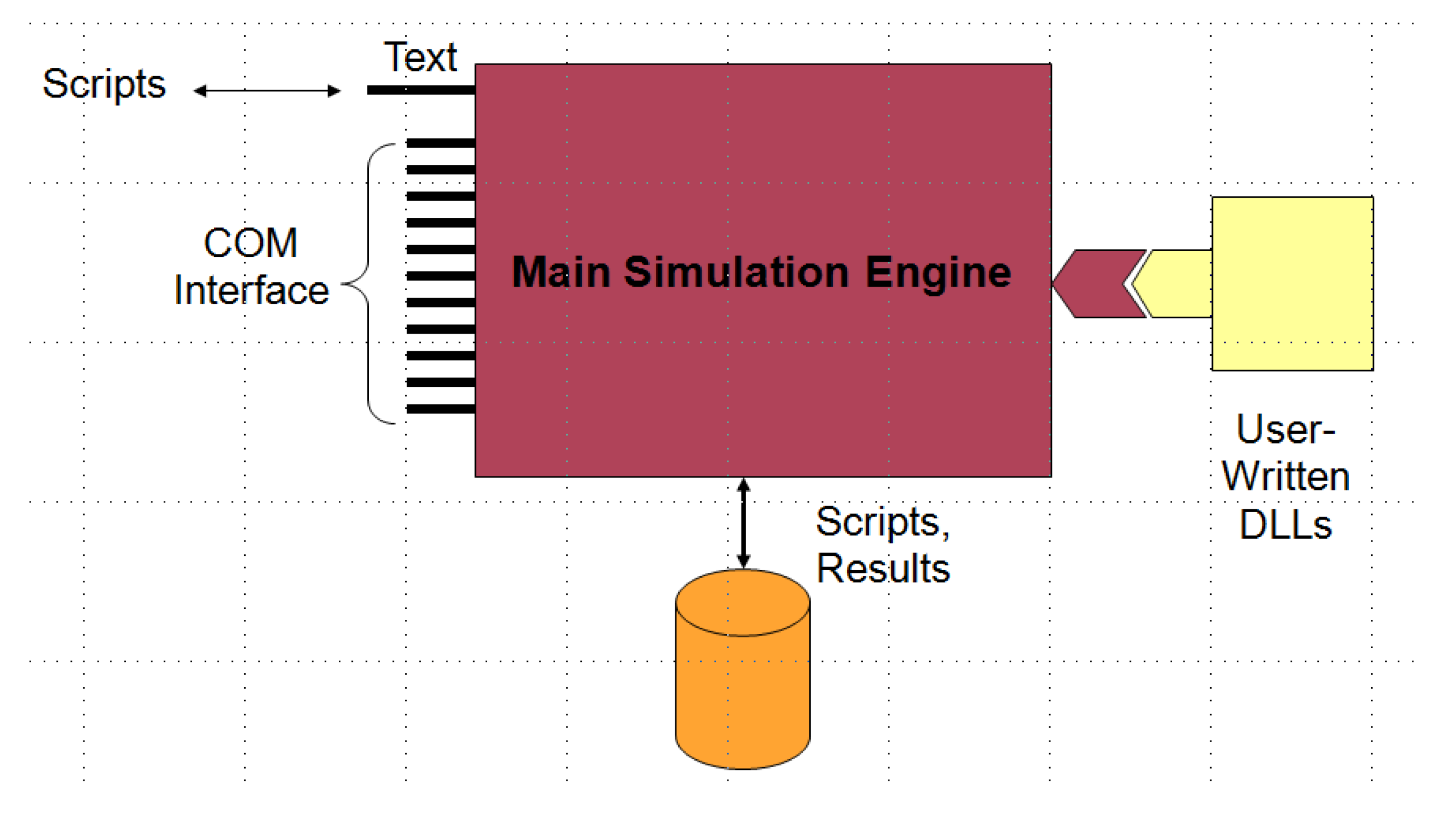
OpenDSS is a comprehensive system simulation tool for electric utility distribution systems, released by the Electric Power Research Institute (EPRI), Palo Alto, California. It is implemented as a stand-alone executable program or can be driven from a variety of existing software platforms that support a component object model (COM) interface. The executable version has a basic text-based user interface on the solution engine to assist users in developing scripts and viewing solutions. The program supports frequency domain analyses commonly performed for utility distribution systems planning and analysis. In addition, it supports many new types of analyses that are designed to meet future needs, many of which are being dictated by the deregulation of utilities worldwide and the initiation of the “smart grid” technologies.

Many of the software features were intended to support distributed generation (DG) analysis needs. Other features support energy efficiency analysis of smart grid applications, power delivery, and also harmonics analysis. The OpenDSS is designed to be expandable so that it can be easily modified to meet future needs. The other way to use OpenDSS is through the COM interface, the user is able to design and execute custom solution modes and features from an external program and perform the functions of the simulator, which includes definition of the model data. Thus, the OpenDSS could be implemented entirely independently of any database or fixed text file circuit definition. For example, it can be driven entirely from a MS Office tool through the visual basic for application (VBA), as we will see in the analysis of this study or from any other 3rd party analysis program that supports the COM interface. Users commonly drive the OpenDSS with MATLAB program, Python, C+, R, and other languages. This provides powerful capabilities and is an excellent way to show the results graph. An overview of the system simulation engine and its interconnection with other programs is shown in Figure 1.

3.2. IEEE 34 Bus Model Development Using OpenDSS

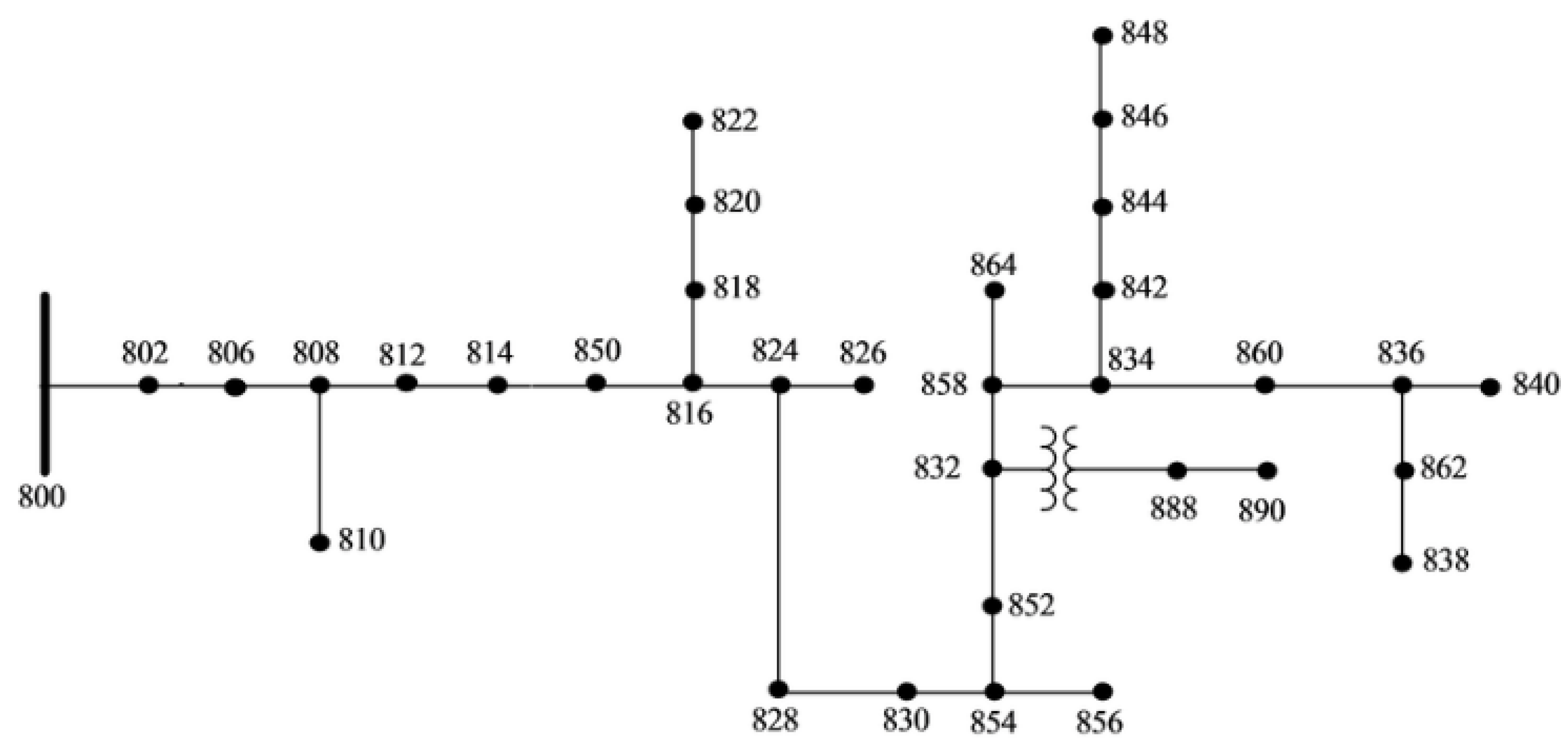
The 34 bus test feeder model, shown in Figure 2, is modeled in this work using the OpenDSS simulator. The system simulation results comparison between OpenDSS, Electrical Distribution Design (EDD), and IEEE standard results are presented in

Table 1. IEEE34bus Model Steady State Data Comparison.

	OpenDSS	EDD	Standard
Total Power MW	2.03247	2.04317	2.0428
Total Reactive Power Mvar	0.28252	0.29214	0.29025
Power Losses MW	0.270494	0.273	0.273049
Reactive Losses Mvar	0.0341963	0.03696	0.034999
Phase 1 Current A	51.507	54.15	51.58
Phase 2 Current A	44.202	46.81	44.57
Phase 3 Current A	40.593	42.98	40.93

[8].

The EV are modeled as a dynamic kW load in the system in the OpenDss. The following equation better describes the amount of energy evaluated by the EV charging and discharging process as a dynamic load, which was assumed in our modelling [23].

$$E_{i, h}=\left(1-d_b\right)E_{i, h-1}+\left(n_{C }{P}_{i, h}{}^C- \frac{P_{i, h}{}^D}{n_D}\right)\Delta t$$

where $E_{i, h}$ is the amount of energy consumed as load by an EV i at an hour h, $d_b$ as the EV’s self-discharge rate, $n_{C }$ and $n_D$ as both the charging and discharging efficiency which could be modeled in the software, $P_{i, h}{}^C$ and $P_{i, h}{}^D$ are the charging and discharging KW of EV i at time period h, respectively. While $\Delta t$ is the time step, modeled in hours.

4. OpenDSS Model Testing Scenarios and Results

In order to test the system and study the effect of adding charging and discharging EVs to the system, we define the following cases:

Case 1: Random EV Load Increase: increase each load (spot or distributed) until bus or system limit (transformer loading, voltage, and line limit) is reached.

Case 2: Distributed Incremental Increases: Increase loads throughout the system in percentage proportion to the load at the bus (spot load only)

Case 3: Random EV load Charging and Discharging Increase: In addition to the charging at the spot bus, this case will have V2G loads at the spot bus to see the maximum kW that can be discharged to the system.

Case 4: Distributed 10% incremental increase of the charging and discharging loads: Increase charging and discharging loads throughout the system in percentage proportion to the load at the bus (spot load only).

In order to decide accurately the additional EVs that we can add to the system each hour, the following limitations are considered during different scenarios studied in this work:

• Transformer Loading Limit: current rating of 100% (normal), current rating of 125% (emergency).
• Voltage limit: minimum and maximum voltage levels are 0.92 pu to 1.08 pu respectively. The limit is calculated on 120 V base as 110–130 V.
• Line Loading Limit: 100% loading condition.

The above criteria are used in determining the level of incremental EVs that can be connected to the test systems. After analyzing different loading scenarios using OpenDSS, we found that the most sensitive parameter is the line voltages since the lines current in the range of 50 A which represents around 25–30% of the lines capacity, whereas the most sensitive buses voltages are shown in

Table 2. Monitored Buses Voltages.

Bus	Base kV	Phase 1 pu	Phase 2 pu	Phase 3 pu
814	24.9	0.94683	0.99543	0.98993
852	24.9	0.96451	0.96954	0.9644
890	4.16	0.92336	0.92513	0.91833

.

The buses above have the lowest voltage profile and as we test our system and add the electric vehicles to the network, these buses should be monitored closely to insure stable operation. In the original case without any additional load, we notice that bus 890 has a low voltage profile and requires voltage support through shunt capacitors or a voltage regulator. As we test the system for different scenarios, we will stop at the next low bus voltage level to see the amount of additional EVs that can be added to the system.

4.1. Load Profile of the Distribution Feeder

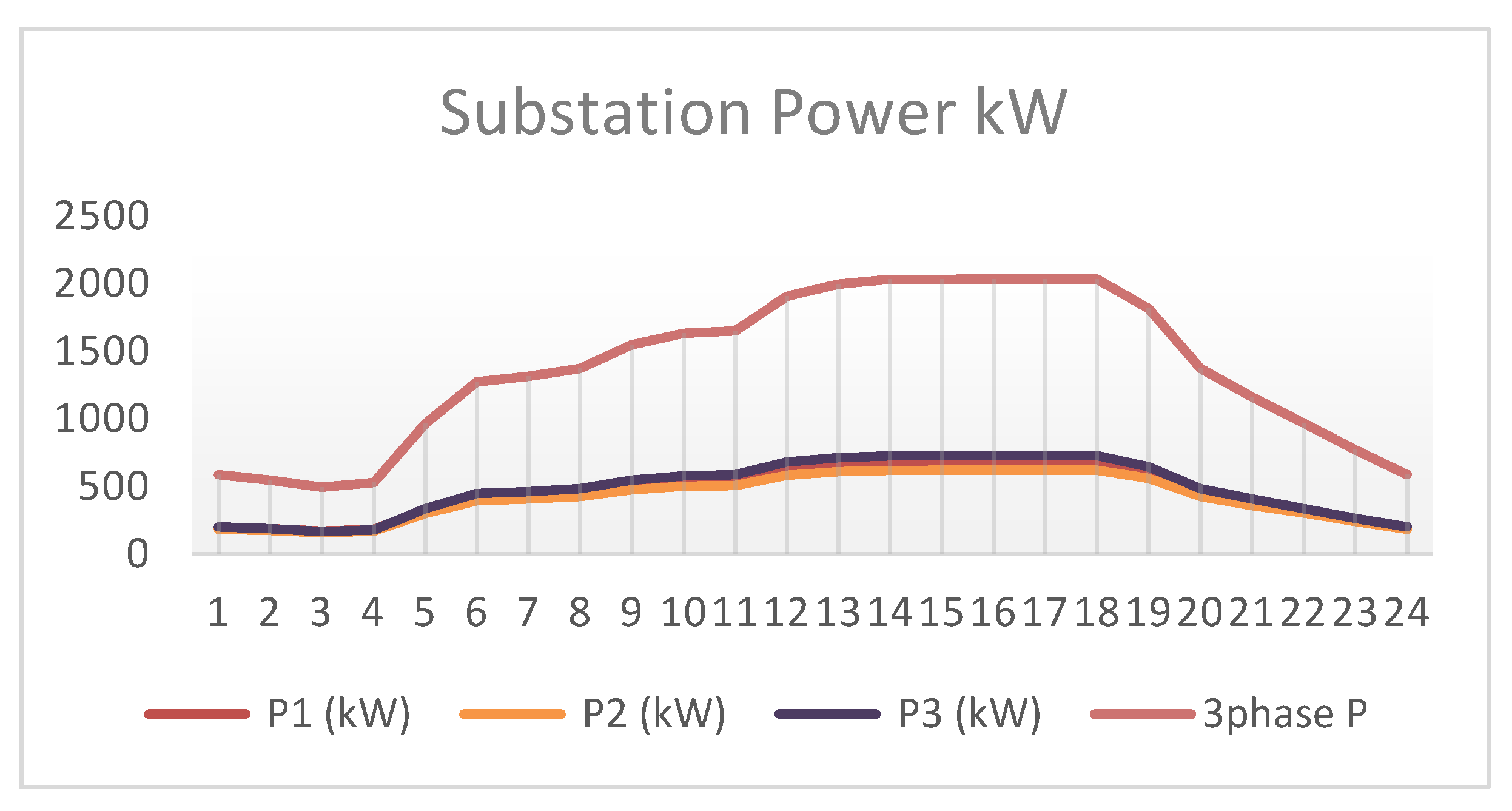
In this work we take into account that the load changes based on the daily time of use and this will affect the amount of EVs that can be added to the system at different times of the day. The way to test the model in OpenDSS is to increase the loads at the specified buses according to the cases. Once the system reaches the maximum limit, the maximum amount of EVs Charging/Discharging for each hour of the day can be decided and the amount of EVs to be connected at that duration is calculated as well. As load changes in Figure 3, the substation power output will vary as expected. The figure shows the substation single-phase power and the total three phase power.

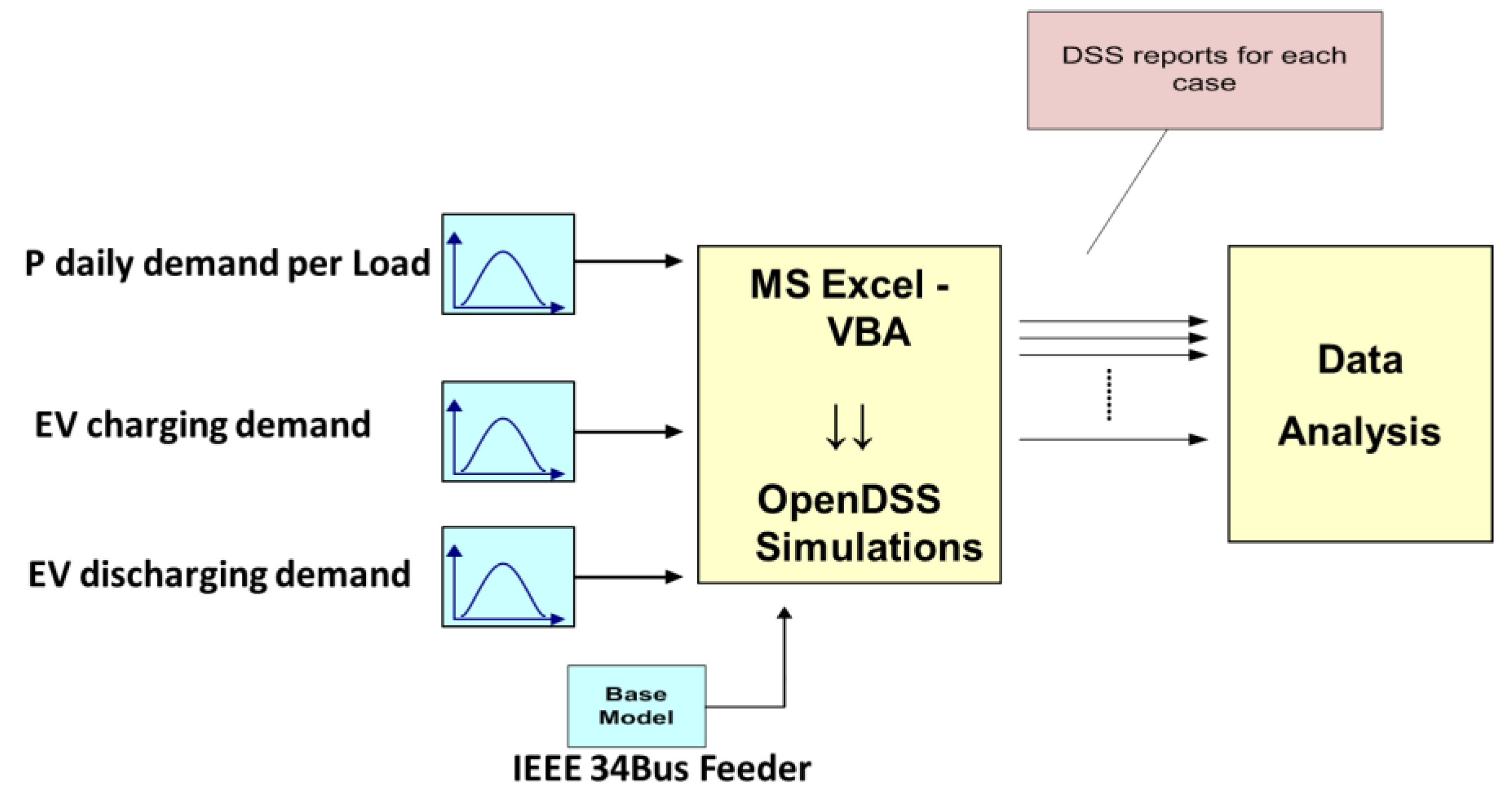
We model the system using OpenDSS by utilizing the COM feature at the simulator to communicate with MS excel and Visual Basic Software to capture the data each hour and arrange it in a readable format and plot each transformer, line, bus, and load data. Figure 4 shows the way we introduce the demand load and EV charging/discharging demand and read the results.

In addition to the amount of kW that can be added to the system, the cost of the additional charging and discharging kW can be calculated to see the effect of the time of use rate on the hourly charging and discharging loads. For this purpose we will use Florida Light and Power’s (FPL) recent time-of-use rates for charging electric vehicles for a more realistic simulation of our work. We have made an assumption that the rate for discharging power to the grid is going to be the same rate. This assumption might not be accurate but for our purposes is necessary to complete the analysis until the final prices are issued by Southern California Edison (SCE). The price of the additional kW will be shown after each case daily power curve. The time-of-use rate used in this study is shown in

Table 3. Florida Light and Power (FPL) Time of Use Rate.

Season, Date and Time	Summer on Peak	Summer off Peak	Winter on Peak	Winter off Peak
	1 June to 1 October	1 June to 1 October	1 October to 1 June	1 October to 1 June
	12:00 PM to 9:00 PM	All Other Time	12:00 PM to 9:00 PM	All Other Time
Total ($/kwh)	0.48964	0.17177	0.35203	0.1667

.

4.2. Model Testing Scenarios and Results Analysis

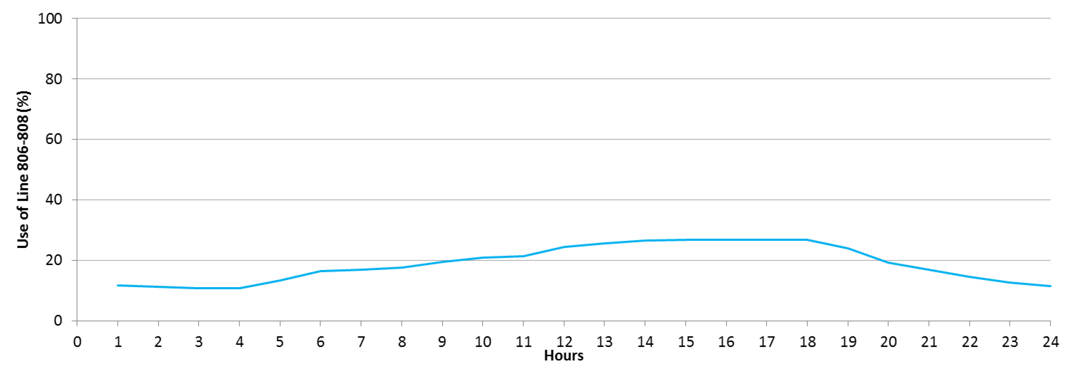
Figure 5 shows a sample of the network lines loading for node 806 to node 808. The utilization is very low and the only option to measure the effect on the system is the voltage profile limit of the line not the loading limit.

Case 1: Random EV Load Increase: Increase each spot load until bus or system limit (transformer loading, voltage, and line limit) is reached

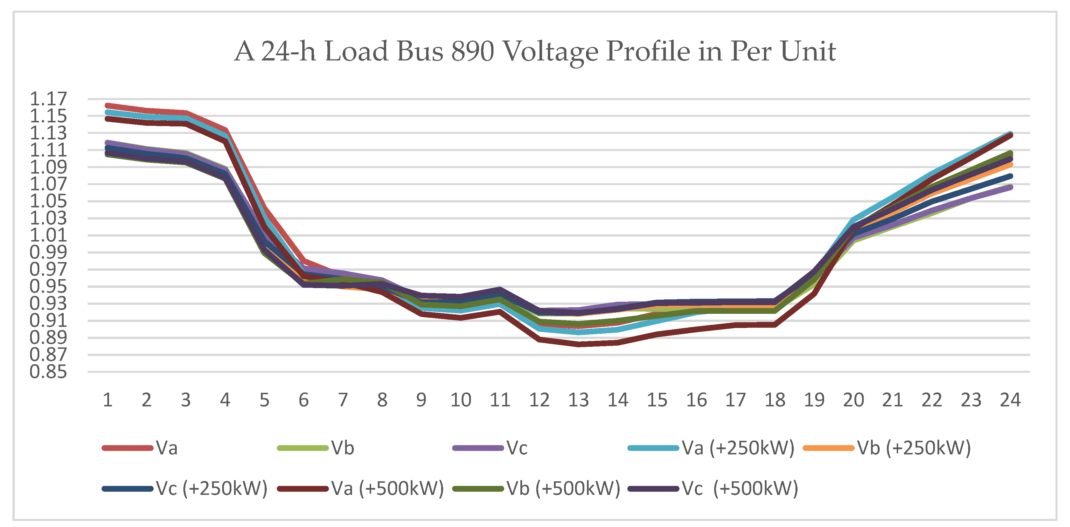
For this case study, we worked on several buses on the system to analyze the effect of adding EVs as random load increases on the system. For the convenience of our work, we show the results of work at spot bus 840. First, we start to increase the amount of additional EVs charging a load to the bus until one of the three buses 890, 852, and 814 reach the lower limit.

Table 4. Case 1 Maximum Additional kW on Bus 840 during Peak Hours.

Bus	Base Case	Additional 250 kW Load on Bus 840	Additional 500 kW Load on Bus 840
890	Below 0.92	Below 0.91	Below 0.90
852	No Violation	No Violation	0.92
814	No Violation	No Violation	0.92

below shows the amount we added to the bus and the per unit voltage at the three buses, while

Table 5. Summary of Case 1 buses Maximum Additional Load.

Spot Load Bus	Additional Load	Bus 890 Voltage pu	Bus 852 Voltage pu	Bus 814 Voltage pu
Bus 840	Original Case	below 0.92	NO Violation	NO Violation
	250 kW	below 0.91	NO Violation	NO Violation
	500 kW	below 0.90	0.92	0.92
Bus 860	Original Case	below 0.92	NO Violation	NO Violation
	250 kW	below 0.90	NO Violation	NO Violation
	500 kW	below 0.89	0.92	0.92
Bus 848	Original Case	below 0.92	NO Violation	NO Violation
	250 kW	below 0.90	NO Violation	NO Violation
	500 kW	below 0.89	0.92	0.92
Bus 844	Original Case	below 0.92	NO Violation	NO Violation
	250 kW	below 0.90	NO Violation	NO Violation
	500 kW	below 0.89	0.92	0.92
Bus 890	Original Case	0.92	NO Violation	NO Violation
	10 kW	0.91	NO Violation	NO Violation
	250 kW	0.83	NO Violation	NO Violation
	400 kW	0.79	0.92	0.92
	500 kW	0.77	0.91	0.92
Bus 830	Original Case	0.92	NO Violation	NO Violation
	250 kW	0.91	NO Violation	NO Violation
	500 kW	0.9	NO Violation	NO Violation
	600 kW	0.89	0.92	0.92

shows the overall results when we model this scenario on several load buses. As the results show, a maximum of 500 kW can be added to the bus without violation at buses 852 and 814. Also, one of the unique features of our study is that we were able to visualize the change of voltage level on each bus for each hour as can be seen in Figure 6, which presents the voltage profile of the load bus 890.

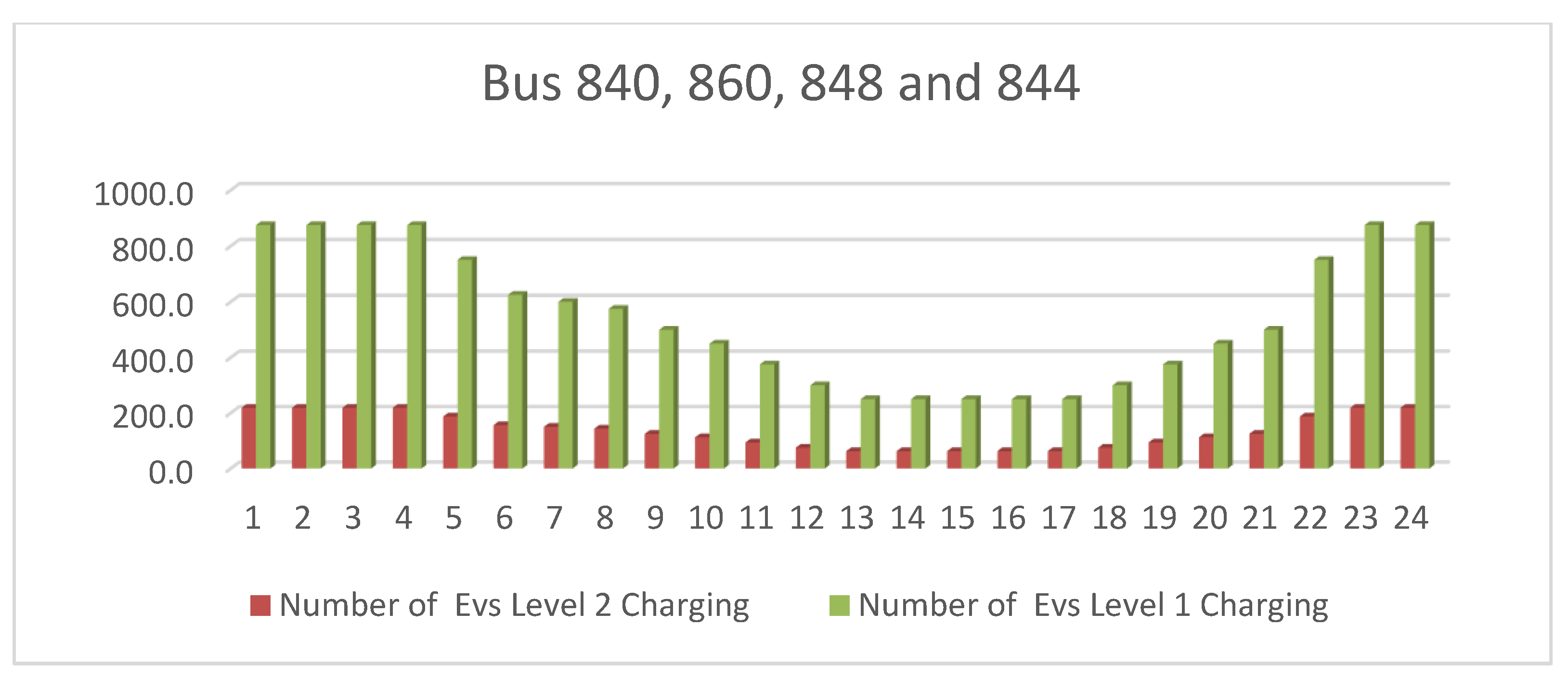
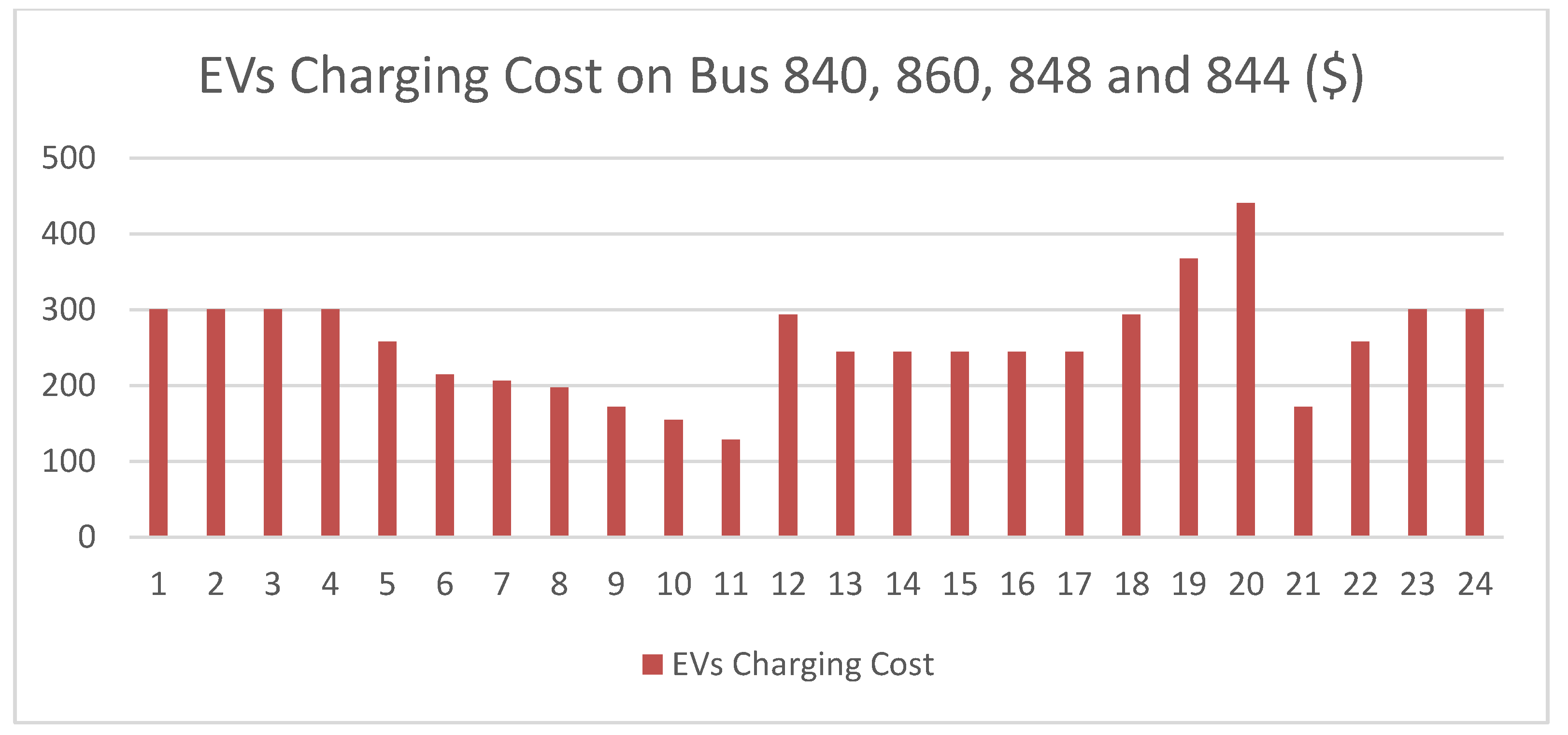
For instance, we assume that load bus 890 requires voltage support by adding a shunt capacitor or voltage regulator, if we consider the next bus to violate and hit system limit, the additional power would be 400 kW. As far as this study, we will not add any additional EV to bus 890 since the bus voltage will be very low (0.79). While other buses performs better as an ideal location for charging/discharging EVs, namely load bus 830, where the maximum power that can be added in period of peak hours (from hour 14 to hour 18) is 600 kW, which is equivalent to 75 EVs with level-2 charging and 300 EVs with level-1 charging. The plan now is to dispatch the EVs as the demand change. The system demand during the off peak periods is low and the system can have additional charging EVs power added to the system. For each hour of the day, we will start to increase the EVs charging load to the buses until we reach the system limit. Figure 7 shows the number of EVs charging into the distribution grid, while Figure 8 shows the costs for adding them based on our use of SCE’s time-of-use rates.

Case 2: Distributed Incremental Increases

For this case, we will start to increase the charging load at the spot buses all together at the same time while 10% of the bus itself loads. The increment will be for all spot buses at the same time. For the peak hours, the maximum load that can be increased is as follows in

Table 6. Case 2 Maximum Charging Load kW during Peak Hours.

Bus	10%	20%	30%	40%	50%
890	0.91	Below 0.91	Below 0.90	Below 0.89	Below 0.88
852	No Violation	No Violation	No Violation	No Violation	Below 0.92
814	No Violation	No Violation	No Violation	No Violation	Below 0.92

, until the system limit is reached.

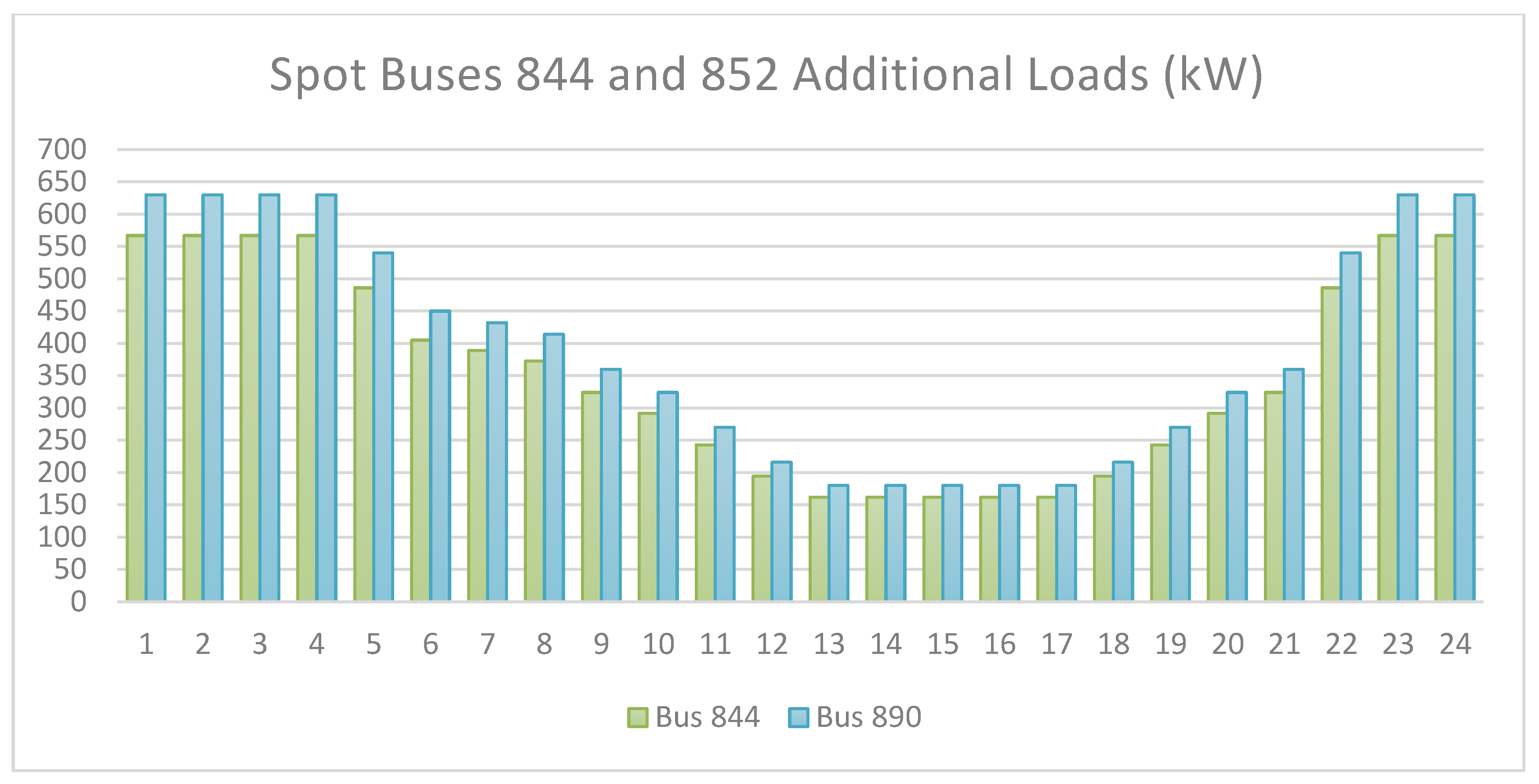
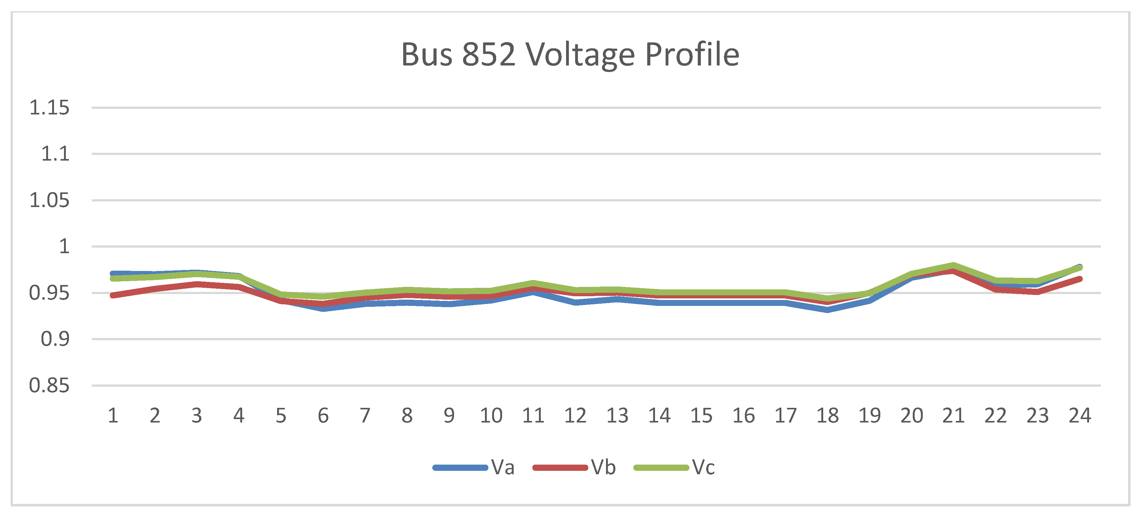
We can increase the spot loads 40% of their original load without any violation on buses 852 and 814. Using a similar process to find the amount of additional load in the previous case, the additional changing load throughout the day was analyzed as well in this paper. Figure 9 shows spot buses 844 and 990 considering additional loads. After adding the different amount of kW at different times of the day, the voltage level at the monitored buses 852 and 814 is almost constant above 0.92 as shown in Figure 10.

Case 3: Random EV load Charging and Discharging Increase

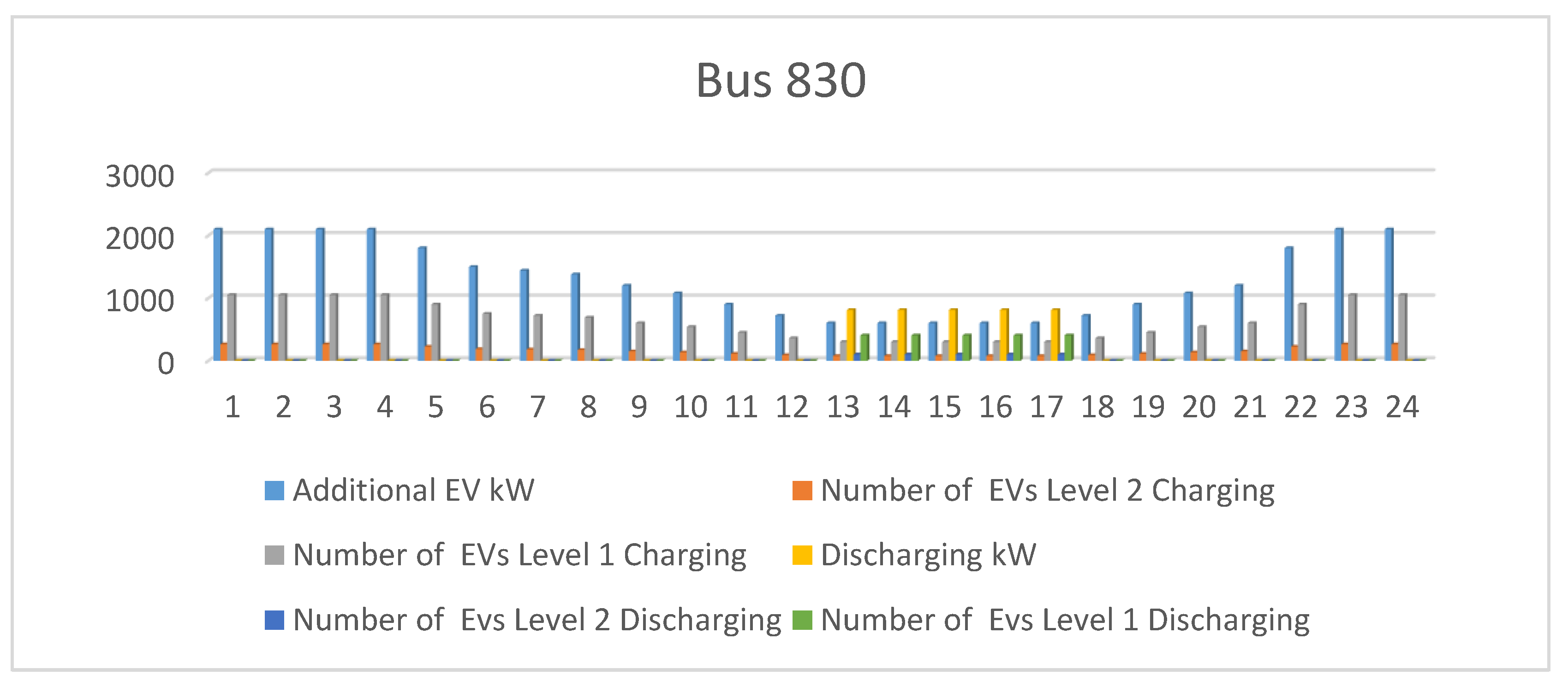
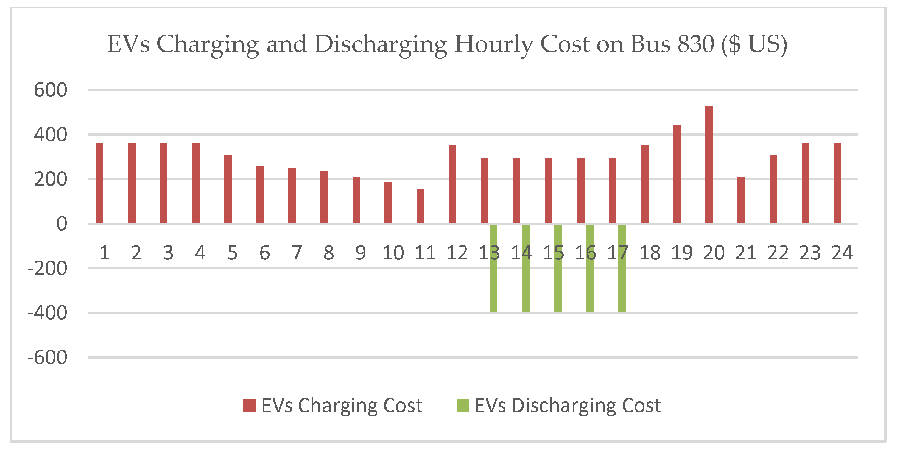
In addition to the charging at the spot bus, this case will have discharging (V2G technology) loads at the spot bus to see the maximum kW that can be discharged to the system. Usually, the discharging will take place when the energy cost is high and during the peak hours. For our study, we consider the discharging process is going to be during the peaking hours to support the system during high load in addition to the maximum charging loads at the spot buses. The results that we obtain should be considered as a good data that can be used for short-term operation planning to quantify the amount of kW that can uphold the system during these hours.

Table 7. Case 3 Maximum Charging/Discharging Load kW during Peak Hours.

Spot Load Bus	EVs Charging kW	EVs Discharging kW	Violation
Bus 840	500	250	No Violation
	500	495	No Violation
	500	500	(Above 1.08 pu) Violation on Buses 832, 834, 842, 840, 844, 846, 848, 858, 860, 862 864
Bus 860	500	250	No Violation
	500	495	No Violation
	500	500	(Above 1.08 pu) Violation on Buses 832, 834, 842, 840, 844, 846, 848, 858, 860, 862 864
Bus 848	500	250	No Violation
	500	495	No Violation
	500	500	(Above 1.08 pu) Violation on Buses 832, 834, 842, 840, 844, 846, 848, 858, 860, 862 864
Bus 844	500	250	No Violation
	500	495	No Violation
	500	500	(Above 1.08 pu) Violation on Buses 832, 834, 842, 840, 844, 846, 848, 858, 860, 862 864
Bus 830	600	250	No Violation
	600	500	No Violation
	600	750	No Violation
	600	810	No Violation
	600	815	(Above 1.08 pu) Violation on Buses 832, 834, 842, 840, 844, 846, 848, 858, 860, 862 864

shows the maximum charging and discharging during the peak hours before any violation to the buses’ voltage level. It is worth mentioning that for the following cases the discharging of the EVs will take place while the maximum number of charging EVs is connected to the system at the same time. This will allow us to see the two bounders of charging loads and discharging loads without reaching the lowest and highest system voltage limits. As the demand changes during the day, the maximum additional charging and discharging load each hour for each spot bus is changed as well based on the grid’s needs. Figure 11 shows the additional charging/discharging and number of EVs connected to load bus 830 (provided as an example for the results obtained in this case). Figure 12 of this work shows the hourly costs based on a real-life TOU rates.

Case 4: Distributed 10% Incremental Increase of the Charging and Discharging Loads

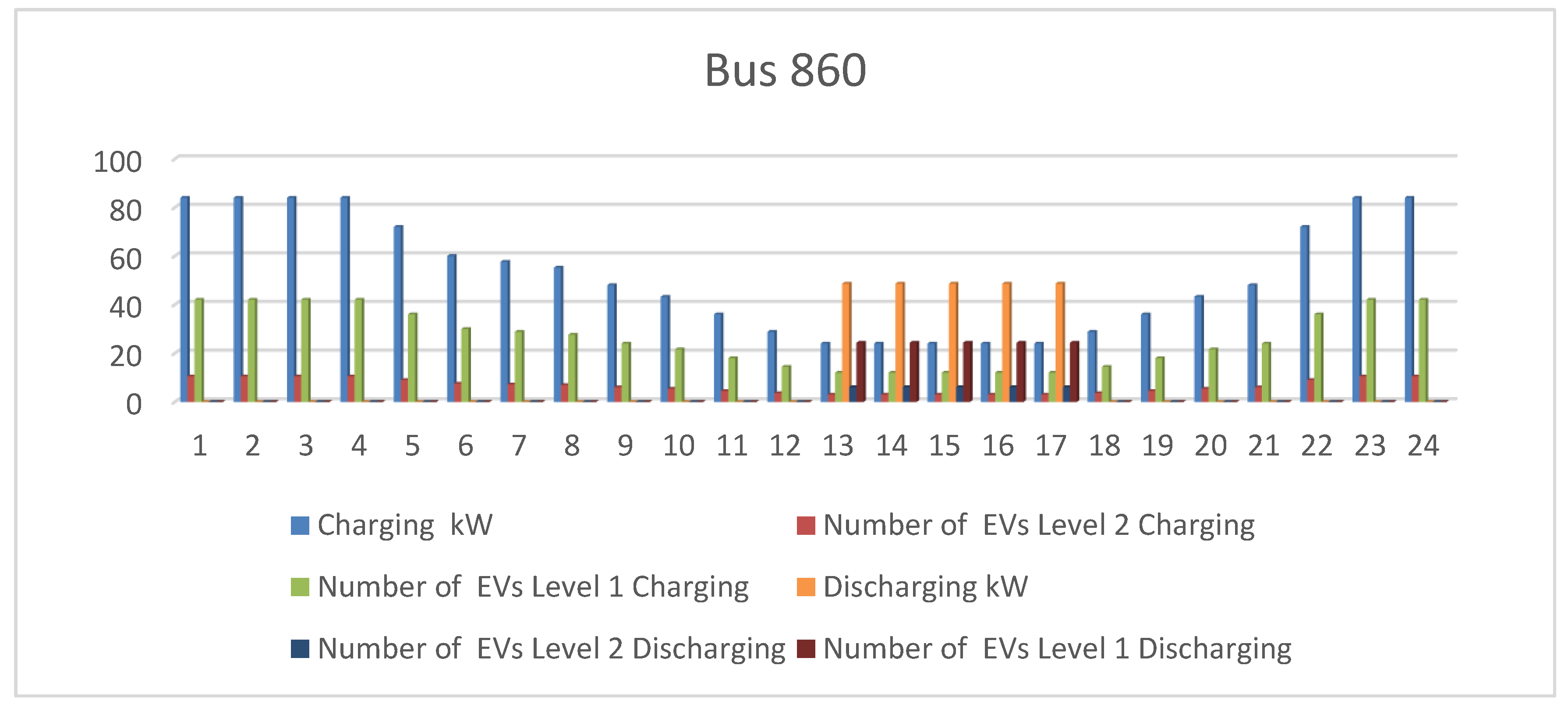
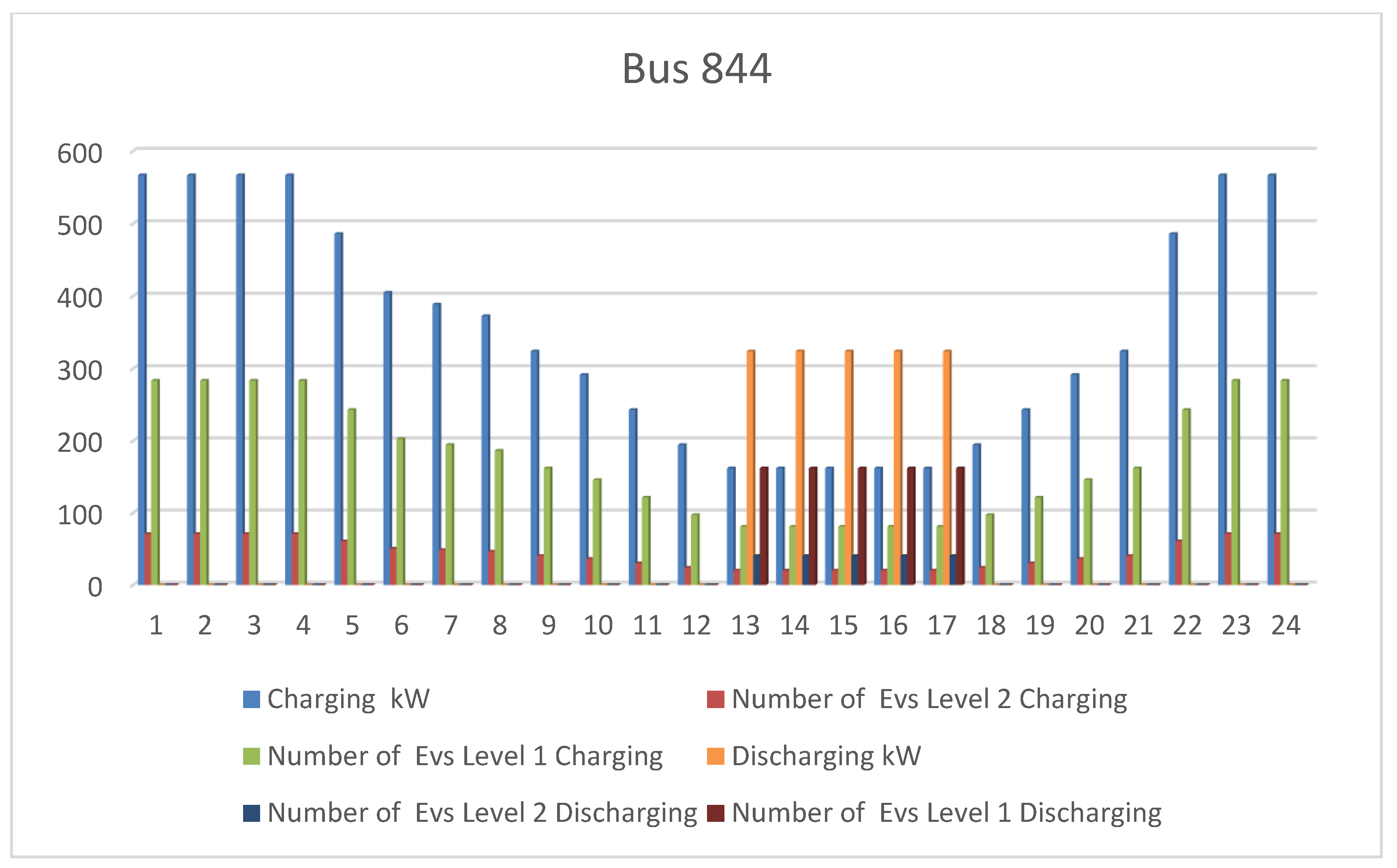
For this case, we increase EVs’ charging and discharging kW throughout the system in percentage proportion to the load at the bus (spot load only). As we saw from case 3, the system will reach the maximum limit if we increase the charging load 40% of the bus total load at certain locations.

Table 8. Case 4 Maximum Charging Load kW during Peak Hours.

Bus	10%	20%	30%	40%	50%
890	0.91	Below 0.91	Below 0.90	Below 0.89	Below 0.88
852	No Violation	No Violation	No Violation	No Violation	Below 0.92
814	No Violation	No Violation	No Violation	No Violation	Below 0.92

shows the results of modeling the distribution feeder in this scenario. For EVs discharging loads, we will start to increase the discharging load at the spot bus until we reach the high limit (1.08 pu) of the voltage level. Such findings allow us to quantify the amount of EVs penetration that can be deployed (with previous agreements) into the system as controllable loads that provide local voltage support to help the operators in minimizing the congestion during peak hours, while enabling more EVs to charge during those hours without causing any voltage dips.

Table 9. Case 4 Maximum Charging/Discharging Load kW during Peak Hours.

Distributed Increase on Spot Buses	EVs Charging Violation	EVs Discharging Violation
10% Charging and 10% Discharging	No Violation	No Violation
20% Charging and 20% Discharging	No Violation	No Violation
30% Charging and 30% Discharging	No Violation	No Violation
40% Charging and 40% Discharging	No Violation	No Violation
50% Charging and 50% Discharging	Violation on bus 814	No Violation
40% Charging and 60% Discharging	No Violation	No Violation
40% Charging and 70% Discharging	No Violation	No Violation
40% Charging and 80% Discharging	No Violation	No Violation
40% Charging and 90% Discharging	No Violation	(Above 1.08 pu) Violation on Buses 832, 834, 842, 840, 844, 846, 848, 858, 860, 862 864

shows the maximum percentage amount increase in discharging load, which is 80% of the spot buses loads. For the different hours of the day other than the peak hours, the charging and discharging loads are simulated in our work. Figure 13 and Figure 14 shows the modelling results for load buses 860 and 844, highlighting the number of EVs that could be charged each hour of the day (both types I and II).

5. Conclusions

This article presents a study to model the impact of Electric Vehicle integration on the hourly performance and operation of the distribution grid. The system’s sensitive parameter to identify violation in our scenarios was the voltage limit not to exceed or degrade from the 8% limit of the bus voltage level. In our study, we modeled the IEEE 34 test system considering all of its parameters, such as transmission line parameters, voltage, line loading capacities and frequency, and transformer connections, as well as considered a real-life 24 h load data to present results that simulate real-life outcomes. We took into consideration the financial variables to model the pricing of EV charging throughout the day based on defined TOU rates for each season of the year. The results show the expected number of EVs that could be connected to charged, or discharge as in cases 3 and 4, in each node of that test system, along with the projected costs to do so. The results show the locations in the system that are in need voltage support throughout the charging process in each hour of the day, as well as point to the most ideal locations to potentially host a charging station to serve the test feeder, as our study quantifies the approximate number of the EVs that could be served on an hourly basis without causing any violation during the normal daily operation.

Table 10. Summary of the different Cases Charging and Discharging Costs.

	Total Charging Energy (kWh)	Total Discharging Energy (kWh)	Net Energy (kWh)	Total Charging Cost ($ US)	Total Discharging Cost ($ US)	Net Cost ($ US)
Case 1 buses 840, 860, 848, 844	26,100	0	26,100	6183.8	0	6183.8
Case 1 bus 830	31,320	0	31,320	7420.56	0	7420.56
Case 2	26,100	0	26,100	6183.8	0	6183.8
Case 3	21,861.36	0	21,861.36	5179.63	0	5179.63
Case 4 buses 840, 860, 848, 844	26,100	2295	23,805	6183.8	−1123.724	5060.076
Case 4 bus 830	31,320	4050	27,270	7420.56	−1983	5437.56
Case 4	21,861.36	4198.5	17,662.86	5179.63	−2055.806	3123.824

below summarizes the different cases of total charging and discharging energy of the day and summarizes the total cost for charging and discharging each case. We can conclude that the additional load on bus 830 for case 1 and case 4 seems to be the best place to have the highest possible energy and eventually the highest number of Electric Vehicles.

References

- Willis, H.L.; Scott, W.G. Distributed Power Generation. Planning and Evaluation; Marcel Dekker: New York, NY, USA, 2000. [Google Scholar]
- Borlease, S. Smart Grids: Infrastructure, Technology and Solutions; CRC Press: Boca Raton, FL, USA, 2013. [Google Scholar]
- The International Energy Agency (IEA). Global EV Outlook: Toward Cross-Modal Electrification. 2018. Available online: https://webstore.iea.org/global-ev-outlook-2018 (accessed on 11 August 2018).
- McDermott, T.E.; Dugan, R.C. Distributed generation impact on reliability and power quality indices. In Proceedings of the Rural Electric Power Conference, Colorado Springs, CO, USA, 5–7 May 2002; Volume D3, pp. 1–7. [Google Scholar]
- Trichakis, P.; Taylor, P.C.; Lyons, P.F.; Hair, R. Predicting the technical impacts of high levels of small-scale embedded generators on low-voltage networks. IET Renew. Power Gener. 2008, 2, 249–262. [Google Scholar] [CrossRef]
- Hadley, S.W. Impact of Plug-In Hybrid Vehicles on the Electric Grid; Technical report ORNL/TM-2006/554; Oak Ridge National Laboratory: Oak Ridge, TN, USA, 2006. [Google Scholar]
- Denholm, P.; Short, W. An Evaluation of Utility System Impacts and Benefits of Optimally Dispatched Plug-In Hybrid Electric Vehicles; Technical report; National Renewable Energy Laboratory: Golden, CO, USA, 2006. [Google Scholar]
- Kersting, W.H. Distribution System Modeling and Analysis; CRC: Boca Raton, FL, USA, 2002. [Google Scholar]
- IEEE 34 Bus Test Feeder. Available online: http://ewh.ieee.org/soc/pes/dsacom/testfeeders/ (accessed on 17 May 2018).
- Williams, B.D.; Kurani, K.S. Commercializing light-duty plugin/plug-out hydrogen-fuel-cell vehicles: ‘Mobile Electricity’ technologies and opportunities. J. Power Sources 2007, 166, 549–566. [Google Scholar] [CrossRef]
- Tomic, J.; Kempton, W. Using fleets of electric-drive vehicles for grid support. J. Power Sources 2007, 168, 459–468. [Google Scholar] [CrossRef]
- Aljohani, T.; Beshir, M. Distribution System Reliability Analysis for Smart Grid Applications. Smart Grid Renew. Energy 2017, 8, 240–251. [Google Scholar] [CrossRef]
- Aljohani, T.; Beshir, M. Matlab Code to Assess the Reliability of the Smart Power Distribution System Using Monte Carlo Simulation. J. Power Energy Eng. 2017, 5, 30–44. [Google Scholar] [CrossRef]
- Aljohani, T.M. The Impact of EPA’s New Proposed Limits on the U.S. Power Industry. Int. J. Electr. Energy 2014, 2, 343–347. [Google Scholar] [CrossRef]
- Eldeeb, H.H.; Faddel, S.; Mohammed, O.A. Multi-Objective Optimization Technique for the Operation of Grid tied PV Powered EV Charging Station. Electr. Power Syst. Res. 2018, 164, 201–211. [Google Scholar] [CrossRef]
- Miceli, R.; Viola, F. Designing a Sustainable University Recharge Area for Electric Vehicles: Technical and Economic Analysis. Energies 2017, 10, 1604. [Google Scholar] [CrossRef]
- Ul-Haq, A.; Cecati, C.; Al-Ammar, E.A. Modeling of a Photovoltaic-Powered Electric Vehicle Charging Station with Vehicle-to-Grid Implementation. Energies 2017, 10, 4. [Google Scholar] [CrossRef]
- Olivella-Rosell, P.; Villafafila-Robles, R.; Sumper, A.; Bergas-Jané, J. Probabilistic Agent-Based Model of Electric Vehicle Charging Demand to Analyse the Impact on Distribution Networks. Energies 2015, 8, 4160–4187. [Google Scholar] [CrossRef] [Green Version]
- Yang, J.; Hao, W.; Chen, L.; Chen, J.; Jin, J.; Wang, F. Risk Assessment of Distribution Networks Considering the Charging-Discharging Behaviors of Electric Vehicles. Energies 2016, 9, 560. [Google Scholar] [CrossRef]
- Cao, C.; Wang, L.; Chen, B. Mitigation of the Impact of High Plug-in Electric Vehicle Penetration on Residential Distribution Grid Using Smart Charging Strategies. Energies 2016, 9, 1024. [Google Scholar] [CrossRef]
- Ebrahim, A.F.; Mohammed, O.A. Pre-Processing of Energy Demand Disaggregation Based Data Mining Techniques for Household Load Demand Forecasting. Inventions 2018, 3, 45. [Google Scholar] [CrossRef]
- Elsayad, N.; Moradisizkoohi, H.; Mohammed, O. Design and Implementation of a New Transformerless Bidirectional DC-DC Converter with Wide Conversion Ratios. IEEE Trans. Ind. Electron. 2018. [Google Scholar] [CrossRef]
- Liu, D.; Wang, Y.; Shen, Y. Electric vehicle charging and discharging coordination on distribution network using multi-objective particle swarm optimization and fuzzy decision making. Energies 2016, 9, 186. [Google Scholar] [CrossRef]
Figure 1.
Open Distribution System Simulator (OpenDSS) Model Setup.
Figure 2.
IEEE34 Bus Feeder Layout.
Figure 3.
Substation Daily Power Demand.
Figure 4.
Study Simulation Block Diagram.
Figure 5.
Buses 806-808 Line Loading Capacity.
Figure 6.
Case 1-1 Bus 890 Voltage (in PU) per Each Hour in the day.
Figure 7.
Case 1 number of EVs on Bus 840, 860, 848 and 844.
Figure 8.
Case 1 Charging Cost on buses 840, 860, 848, and 844.
Figure 9.
Case 2 Spot Buses 844 and 890 Additional Loads (kW).
Figure 10.
Case 2 Bus 852 Voltage Profile (in Pu) after adding the charging load.
Figure 11.
Case 3 Additional Charging/Discharging Load and number of EVs on Bus 830.
Figure 12.
Case 3 EVs Charging and Discharging Cost on Bus 830.
Figure 13.
Case 4 Additional Charging/Discharging Load and Number of EVs on Bus 860.
Figure 14.
Case 4 Additional Charging/Discharging Load and Number of EVs on Bus 844.