
Land Cover Classification in the Antioquia Region of the Tropical Andes Using NICFI Satellite Data Program Imagery and Semantic Segmentation Techniques


Abstract
:1. Introduction
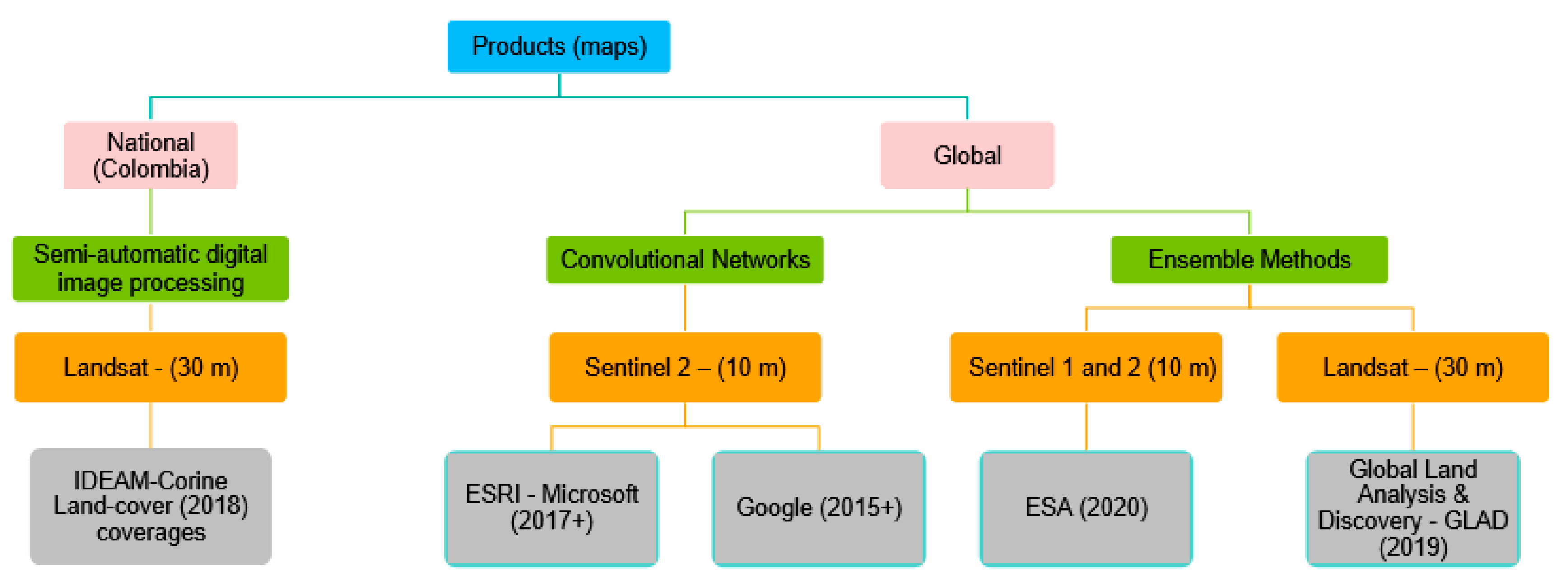
2. Previous Work
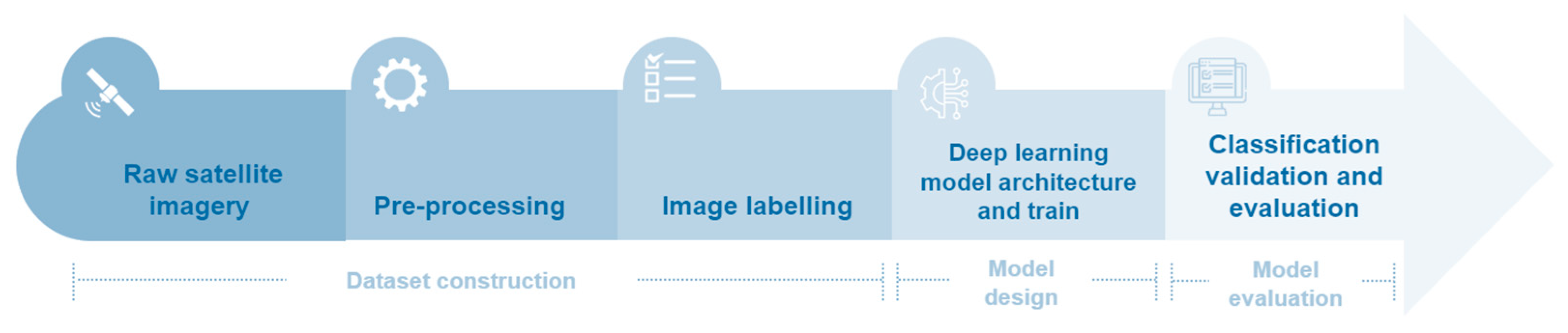
3. Materials and Methods
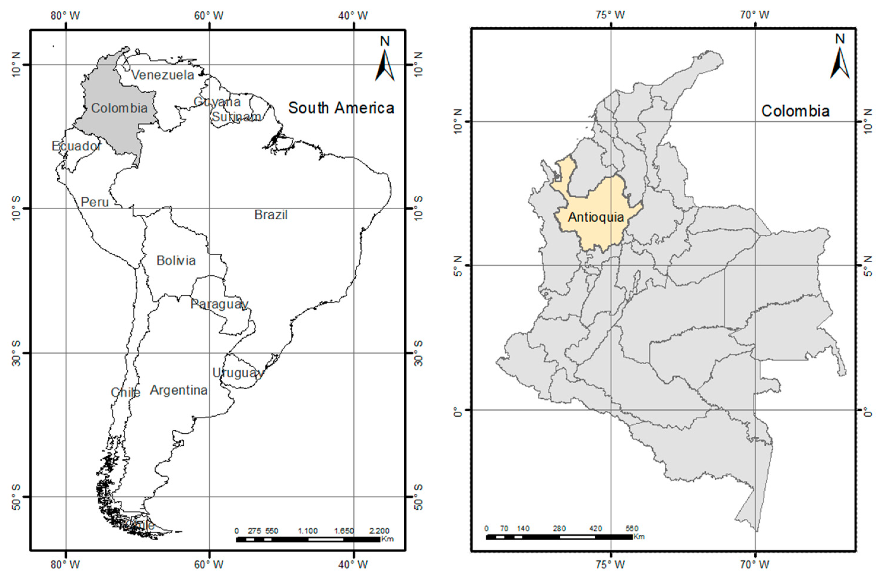
3.1. Study Area Definition
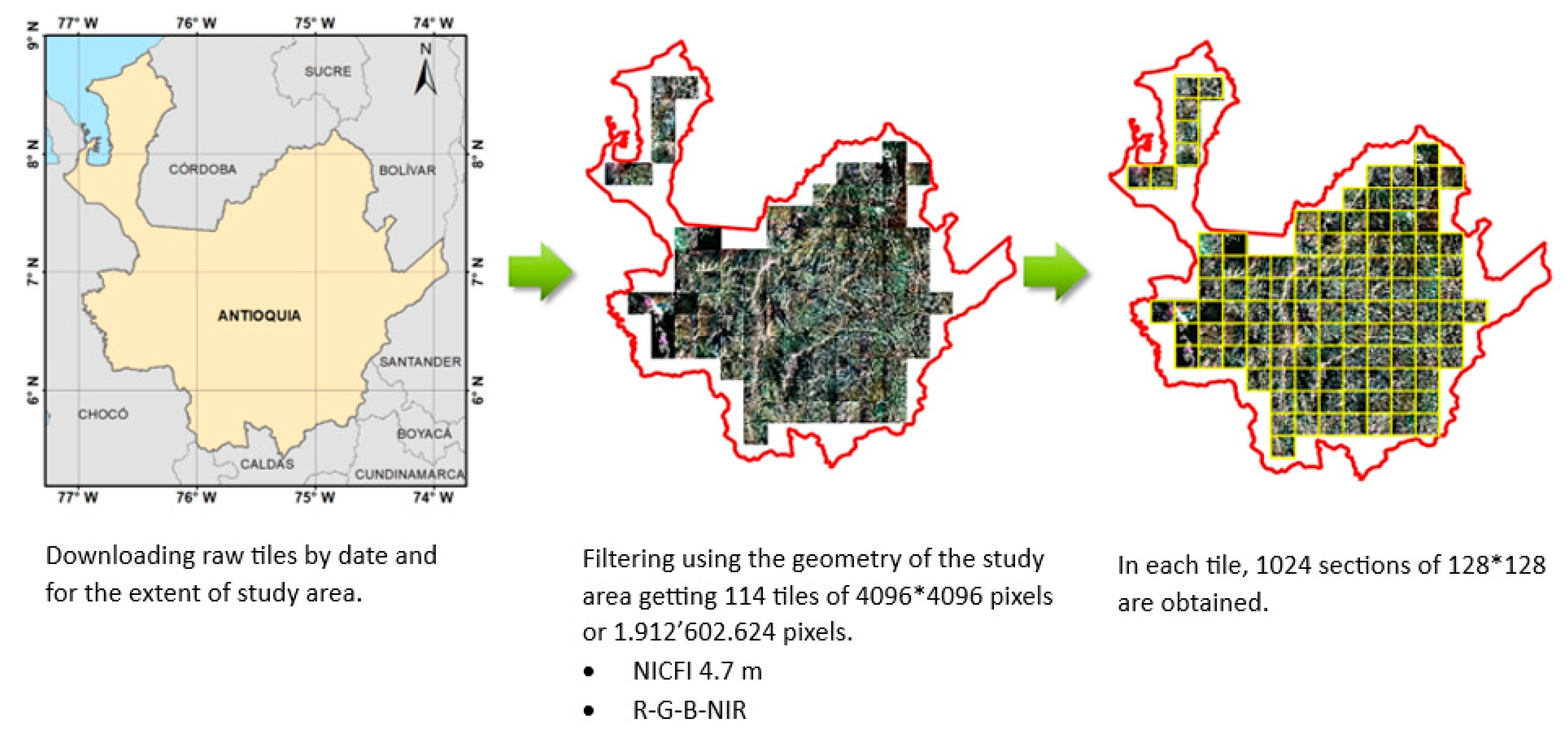
3.2. Raw Satellite Imagery
3.3. Preprocessing
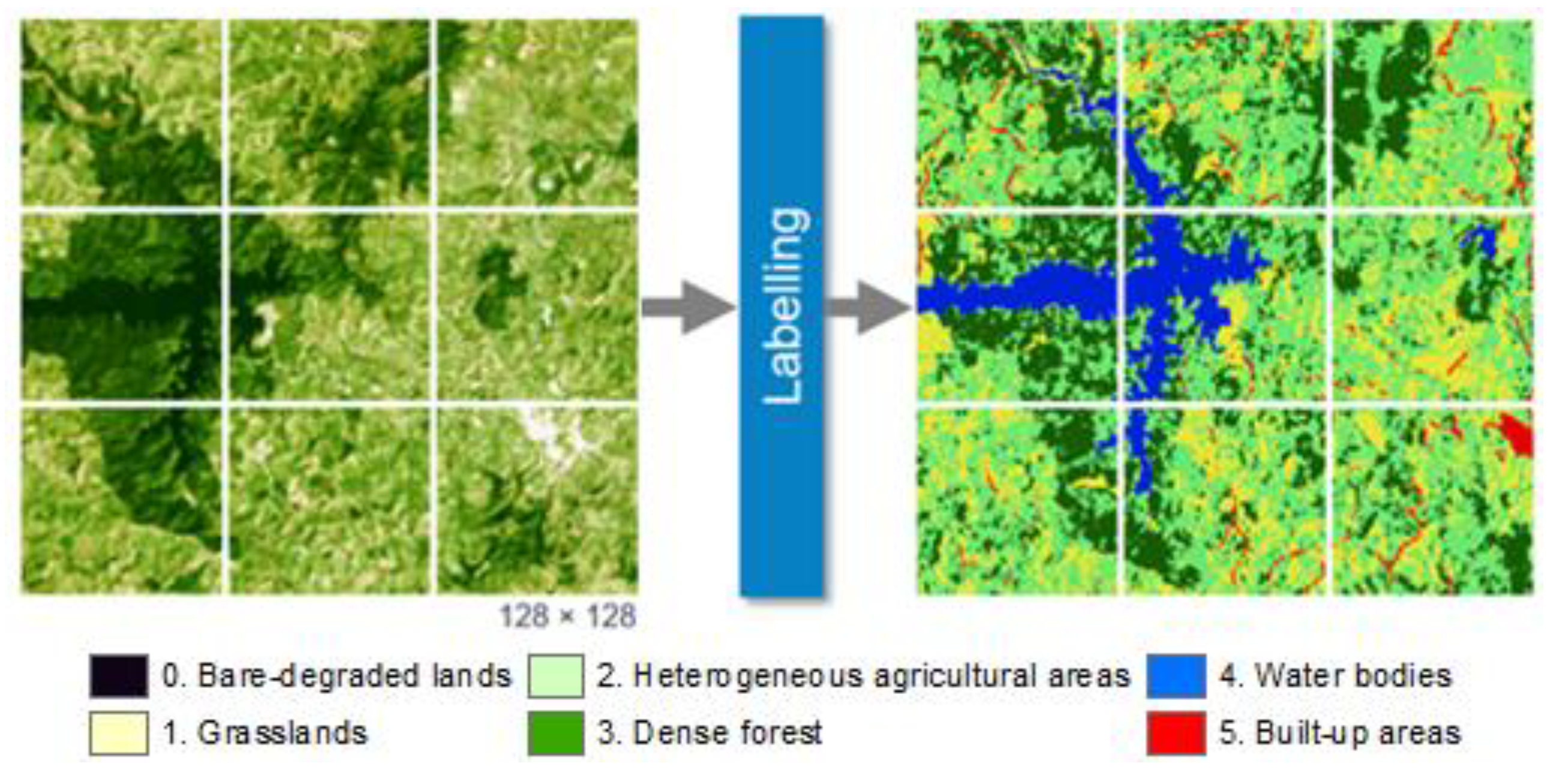
3.3.1. Image Labelling
- Bare-degraded land: corresponds to terrain surfaces devoid of vegetation or with scant vegetation cover due to the occurrence of natural and human-induced processes.
- Dense forest: corresponds to a vegetation community dominated by typical tree elements, which form a continuous or semi-continuous canopy.
- Agricultural heterogeneous areas: corresponds to areas dedicated to permanent, transient, and mixed crops with natural spaces, such as open tree cover.
- Grasslands: corresponds to lands where pastures have been structured with little vegetation presence.
- Water bodies: corresponds to permanent bodies of water.
- Built-up areas: corresponds to territories covered by urban areas, including parks and urban green areas.
3.3.2. Construction of Balanced Dataset
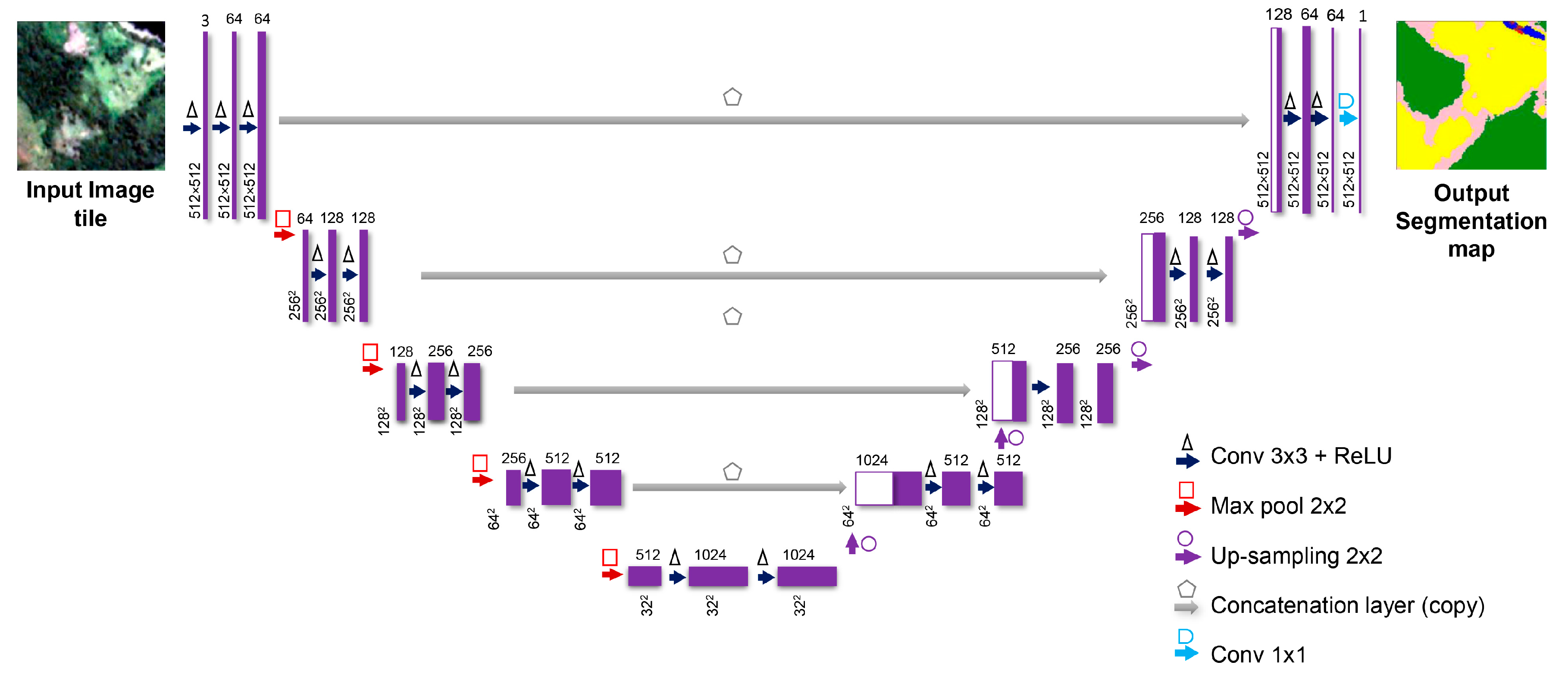
3.4. Deep Learnig Model Architecture and Train
3.5. Classification Validation and Evaluation
4. Results
4.1. Image Labelling
- Bare-degraded lands: 0.61%
- Dense forest: 48.65%
- Heterogeneous agricultural areas: 22.66%
- Grasslands: 25.8%
- Water bodies: 1.09%
- Built-up areas: 1.20%
4.2. Balanced Dataset
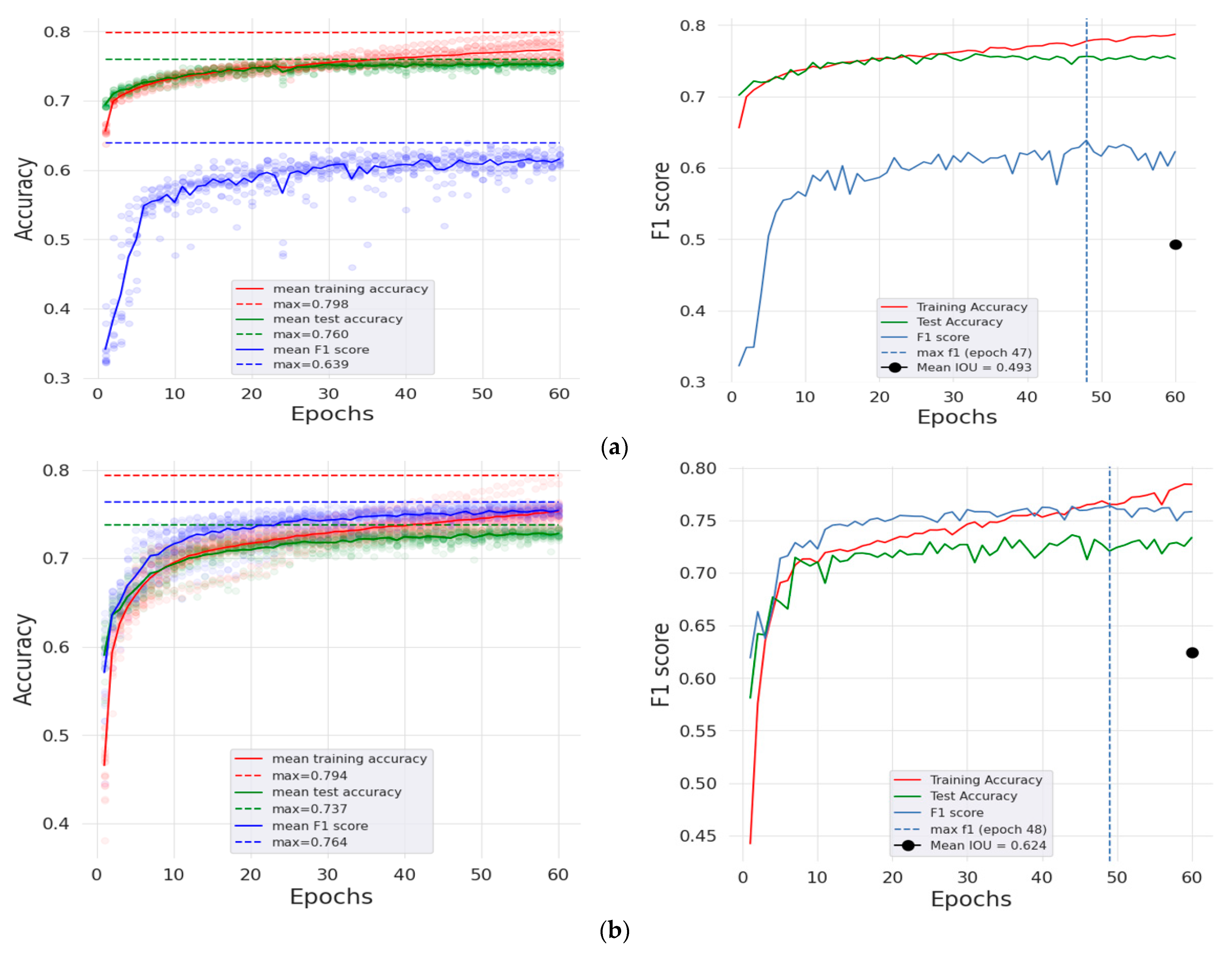
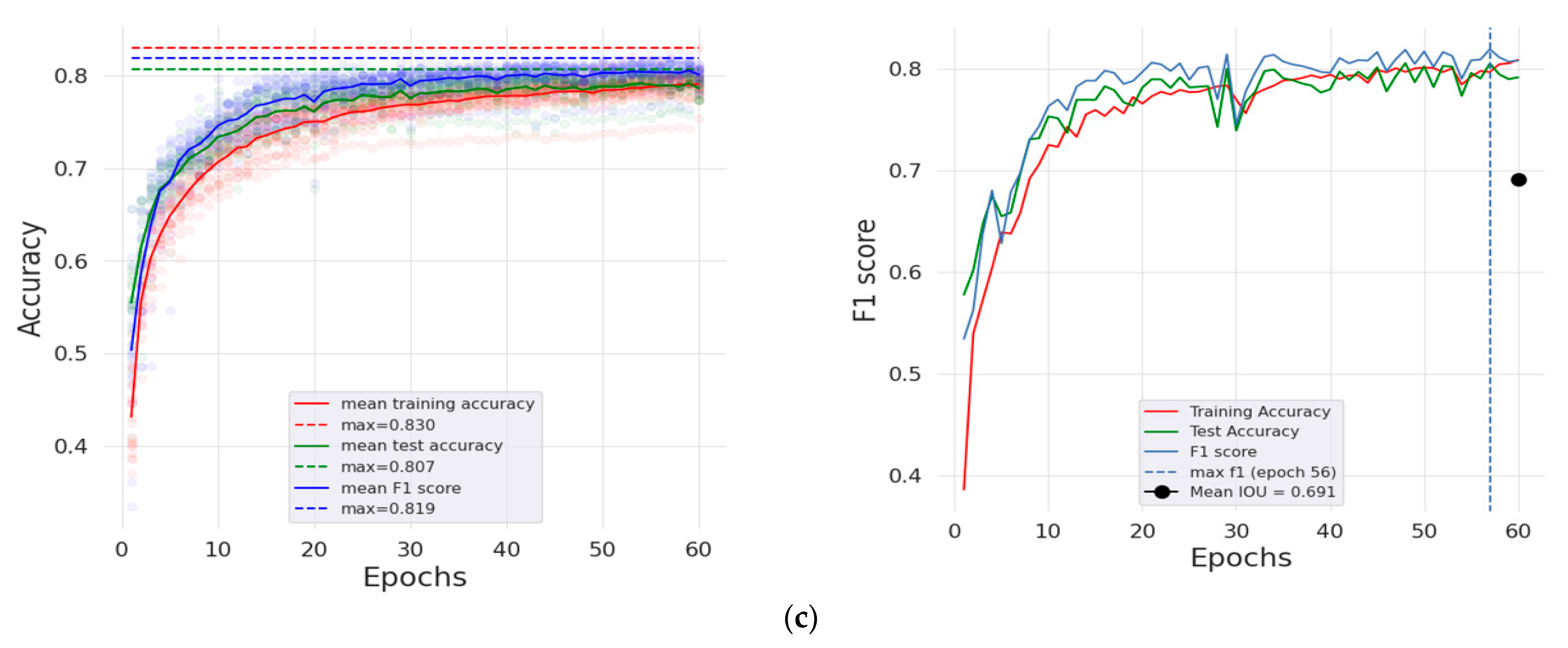
4.3. Model Training
5. Discussion
5.1. Dataset Generation
- 0. Bare-degraded land
- 1. Grasslands
- 2. Agricultural heterogeneous areas
- 3. Dense forest
- 4. Water bodies
- 5. Built-up areas
5.2. Practical Application of the Dataset
6. Conclusions
Author Contributions
Funding
Institutional Review Board Statement
Informed Consent Statement
Data Availability Statement
Acknowledgments
Conflicts of Interest
References
- Lalitha, V.; Latha, B. A Review on Remote Sensing Imagery Augmentation Using Deep Learning. Mater. Today Proc. 2022, 62, 4772–4778. [Google Scholar] [CrossRef]
- Yuan, X.; Shi, J.; Gu, L. A Review of Deep Learning Methods for Semantic Segmentation of Remote Sensing Imagery. Expert Syst. Appl. 2021, 169, 114417. [Google Scholar] [CrossRef]
- Singh, S.; Reddy, C.S.; Pasha, S.V.; Dutta, K.; Saranya, K.R.L.; Satish, K.V. Modeling the Spatial Dynamics of Deforestation and Fragmentation Using Multi-Layer Perceptron Neural Network and Landscape Fragmentation Tool. Ecol. Eng. 2017, 99, 543–551. [Google Scholar] [CrossRef]
- Zhang, B.; Li, W.; Zhang, C. Analyzing Land Use and Land Cover Change Patterns and Population Dynamics of Fast-Growing US Cities: Evidence from Collin County, Texas. Remote Sens. Appl. Soc. Environ. 2022, 27, 100804. [Google Scholar] [CrossRef]
- Darem, A.A.; Alhashmi, A.A.; Almadani, A.M.; Alanazi, A.K.; Sutantra, G.A. Development of a Map for Land Use and Land Cover Classification of the Northern Border Region Using Remote Sensing and GIS. Egypt. J. Remote Sens. Space Sci. 2023, 26, 341–350. [Google Scholar] [CrossRef]
- Hosseiny, B.; Abdi, A.M.; Jamali, S. Urban Land Use and Land Cover Classification with Interpretable Machine Learning—A Case Study Using Sentinel-2 and Auxiliary Data. Remote Sens. Appl. Soc. Environ. 2022, 28, 100843. [Google Scholar] [CrossRef]
- Parente, L.; Taquary, E.; Silva, A.P.; Souza, C.; Ferreira, L. Next Generation Mapping: Combining Deep Learning, Cloud Computing, and Big Remote Sensing Data. Remote Sens. 2019, 11, 2881. [Google Scholar] [CrossRef]
- Hermosilla, T.; Wulder, M.A.; White, J.C.; Coops, N.C. Land Cover Classification in an Era of Big and Open Data: Optimizing Localized Implementation and Training Data Selection to Improve Mapping Outcomes. Remote Sens. Environ. 2022, 268, 112780. [Google Scholar] [CrossRef]
- Anderson, K.; Ryan, B.; Sonntag, W.; Kavvada, A.; Friedl, L. Earth Observation in Service of the 2030 Agenda for Sustainable Development. Geo-Spat. Inf. Sci. 2017, 20, 77–96. [Google Scholar] [CrossRef]
- Holloway, J.; Mengersen, K. Statistical Machine Learning Methods and Remote Sensing for Sustainable Development Goals: A Review. Remote Sens. 2018, 10, 1365. [Google Scholar] [CrossRef]
- Helber, P.; Bischke, B.; Dengel, A.; Borth, D. EuroSAT: A Novel Dataset and Deep Learning Benchmark for Land Use and Land Cover Classification. IEEE J. Sel. Top. Appl. Earth Obs. Remote Sens. 2019, 12, 2217–2226. [Google Scholar] [CrossRef]
- Ma, L.; Liu, Y.; Zhang, X.; Ye, Y.; Yin, G.; Johnson, B.A. Deep Learning in Remote Sensing Applications: A Meta-Analysis and Review. ISPRS J. Photogramm. Remote Sens. 2019, 152, 166–177. [Google Scholar] [CrossRef]
- Potsdam, I. 2D Semantic Labeling Contest—Potsdam 2019. ISPRS Potsdam 2D Semantic Labeling Dataset. Available online: https://www.isprs.org/education/benchmarks/UrbanSemLab/2d-sem-label-potsdam.aspx (accessed on 24 June 2023).
- Báez, S.; Jaramillo, L.; Cuesta, F.; Donoso, D.A. Effects of Climate Change on Andean Biodiversity: A Synthesis of Studies Published until 2015. Neotrop. Biodivers. 2016, 2, 181–194. [Google Scholar] [CrossRef]
- Zalles, V.; Hansen, M.C.; Potapov, P.V.; Parker, D.; Stehman, S.V.; Pickens, A.H.; Parente, L.L.; Ferreira, L.G.; Song, X.-P.; Hernandez-Serna, A.; et al. Rapid Expansion of Human Impact on Natural Land in South America since 1985. Sci. Adv. 2021, 7, eabg1620. [Google Scholar] [CrossRef] [PubMed]
- Pérez-Escobar, O.A.; Zizka, A.; Bermúdez, M.A.; Meseguer, A.S.; Condamine, F.L.; Hoorn, C.; Hooghiemstra, H.; Pu, Y.; Bogarín, D.; Boschman, L.M.; et al. The Andes through Time: Evolution and Distribution of Andean Floras. Trends Plant Sci. 2022, 27, 364–378. [Google Scholar] [CrossRef]
- Schmitt, M.; Hughes, L.H.; Qiu, C.; Zhu, X.X. SEN12MS—A Curated Dataset of Georeferenced Multi-Spectral Sentinel-1/2 Imagery for Deep Learning and Data Fusion. arXiv 2019, arXiv:1906.07789. [Google Scholar] [CrossRef]
- Sumbul, G.; Charfuelan, M.; Demir, B.; Markl, V. Bigearthnet: A Large-Scale Benchmark Archive for Remote Sensing Image Understanding. In Proceedings of the IGARSS 2019—2019 IEEE International Geoscience and Remote Sensing Symposium 2019, Yokohama, Japan, 28 July–2 August 2019; pp. 5901–5904. [Google Scholar]
- Qi, X.; Zhu, P.; Wang, Y.; Zhang, L.; Peng, J.; Wu, M.; Chen, J.; Zhao, X.; Zang, N.; Mathiopoulos, P.T. MLRSNet: A Multi-Label High Spatial Resolution Remote Sensing Dataset for Semantic Scene Understanding. arXiv 2020, arXiv:2010.00243. [Google Scholar] [CrossRef]
- Zhu, Q.; Deng, W.; Zheng, Z.; Zhong, Y.; Guan, Q.; Lin, W.; Zhang, L.; Li, D. A Spectral-Spatial-Dependent Global Learning Framework for Insufficient and Imbalanced Hyperspectral Image Classification. IEEE Trans. Cybern. 2022, 52, 11709–11723. [Google Scholar] [CrossRef]
- Mao, L.; Zheng, Z.; Meng, X.; Zhou, Y.; Zhao, P.; Yang, Z.; Long, Y. Large-Scale Automatic Identification of Urban Vacant Land Using Semantic Segmentation of High-Resolution Remote Sensing Images. Landsc. Urban Plan. 2022, 222, 104384. [Google Scholar] [CrossRef]
- Yeung, H.W.F.; Zhou, M.; Chung, Y.Y.; Moule, G.; Thompson, W.; Ouyang, W.; Cai, W.; Bennamoun, M. Deep-Learning-Based Solution for Data Deficient Satellite Image Segmentation. Expert Syst. Appl. 2022, 191, 116210. [Google Scholar] [CrossRef]
- ISPRS Vaihingen 2D Semantic Labeling Dataset. Available online: https://www.isprs.org/education/benchmarks/UrbanSemLab/2d-sem-label-vaihingen.aspx (accessed on 24 June 2023).
- Van Etten, A. Satellite Imagery Multiscale Rapid Detection with Windowed Networks. In Proceedings of the 2019 IEEE Winter Conference on Applications of Computer Vision (WACV), Waikoloa, HI, USA, 7–11 January 2019; pp. 735–743. [Google Scholar]
- Toker, A.; Kondmann, L.; Weber, M.; Eisenberger, M.; Camero, A.; Hu, J.; Hoderlein, A.P.; Şenaras, Ç.; Davis, T.; Cremers, D.; et al. DynamicEarthNet: Daily Multi-Spectral Satellite Dataset for Semantic Change Segmentation. In Proceedings of the 2022 IEEE/CVF Conference on Computer Vision and Pattern Recognition (CVPR), New Orleans, LA, USA, 18–24 June 2022; pp. 21126–21135. [Google Scholar]
- Brown, C.F.; Brumby, S.P.; Guzder-Williams, B.; Birch, T.; Hyde, S.B.; Mazzariello, J.; Czerwinski, W.; Pasquarella, V.J.; Haertel, R.; Ilyushchenko, S.; et al. Dynamic World, Near Real-Time Global 10 m Land Use Land Cover Mapping. Sci. Data 2022, 9, 251. [Google Scholar] [CrossRef]
- Zanaga, D.; Van De Kerchove, R.; De Keersmaecker, W.; Souverijns, N.; Brockmann, C.; Quast, R.; Wevers, J.; Grosu, A.; Paccini, A.; Vergnaud, S.; et al. ESA WorldCover 10 m 2020 V100. Zenodo 2021. [Google Scholar]
- Bragagnolo, L.; da Silva, R.V.; Grzybowski, J.M.V. Amazon and Atlantic Forest Image Datasets for Semantic Segmentation. Zenodo 2021. [Google Scholar] [CrossRef]
- De Moreno, G.M.S.; de Júnior, O.A.C.; de Carvalho, O.L.F.; Andrade, T.C. Deep Semantic Segmentation of Mangroves in Brazil Combining Spatial, Temporal, and Polarization Data from Sentinel-1 Time Series. Ocean Coast. Manag. 2023, 231, 106381. [Google Scholar] [CrossRef]
- Edgeworth, F.Y. On the Probable Errors of Frequency-Constants (Contd.). J. R. Stat. Soc. 1908, 71, 499–512. [Google Scholar] [CrossRef]
- Shivakumar, B.R.; Rajashekararadhya, S.V. Investigation on Land Cover Mapping Capability of Maximum Likelihood Classifier: A Case Study on North Canara, India. Procedia Comput. Sci. 2018, 143, 579–586. [Google Scholar] [CrossRef]
- Mollick, T.; Azam, M.G.; Karim, S. Geospatial-Based Machine Learning Techniques for Land Use and Land Cover Mapping Using a High-Resolution Unmanned Aerial Vehicle Image. Remote Sens. Appl. Soc. Environ. 2023, 29, 100859. [Google Scholar] [CrossRef]
- Sam, S.C.; Balasubramanian, G. Spatiotemporal Detection of Land Use/Land Cover Changes and Land Surface Temperature Using Landsat and MODIS Data across the Coastal Kanyakumari District, India. Geod. Geodyn. 2023, 14, 172–181. [Google Scholar] [CrossRef]
- Otukei, J.R.; Blaschke, T. Land Cover Change Assessment Using Decision Trees, Support Vector Machines and Maximum Likelihood Classification Algorithms. Int. J. Appl. Earth Obs. Geoinf. 2010, 12, S27–S31. [Google Scholar] [CrossRef]
- Saha, S.; Saha, M.; Mukherjee, K.; Arabameri, A.; Ngo, P.T.T.; Paul, G.C. Predicting the Deforestation Probability Using the Binary Logistic Regression, Random Forest, Ensemble Rotational Forest, REPTree: A Case Study at the Gumani River Basin, India. Sci. Total Environ. 2020, 730, 139197. [Google Scholar] [CrossRef]
- Mangkhaseum, S.; Hanazawa, A. Comparison of Machine Learning Classifiers for Land Cover Changes Using Google Earth Engine. In Proceedings of the 2021 IEEE International Conference on Aerospace Electronics and Remote Sensing Technology (ICARES), Bali, Indonesia, 3–4 November 2021; pp. 1–7. [Google Scholar]
- Garg, R.; Kumar, A.; Bansal, N.; Prateek, M.; Kumar, S. Semantic Segmentation of PolSAR Image Data Using Advanced Deep Learning Model. Sci. Rep. 2021, 11, 15365. [Google Scholar] [CrossRef]
- Palanisamy, P.A.; Jain, K.; Bonafoni, S. Machine Learning Classifier Evaluation for Different Input Combinations: A Case Study with Landsat 9 and Sentinel-2 Data. Remote Sens. 2023, 15, 3241. [Google Scholar] [CrossRef]
- Yuh, Y.G.; Tracz, W.; Matthews, H.D.; Turner, S.E. Application of Machine Learning Approaches for Land Cover Monitoring in Northern Cameroon. Ecol. Inform. 2023, 74, 101955. [Google Scholar] [CrossRef]
- Breiman, L. Random Forests. Mach. Learn. 2001, 45, 5–32. [Google Scholar] [CrossRef]
- Valle, T.M.D.; Jiang, P. Comparison of Common Classification Strategies for Large-Scale Vegetation Mapping over the Google Earth Engine Platform. Int. J. Appl. Earth Obs. Geoinf. 2022, 115, 103092. [Google Scholar] [CrossRef]
- Zhang, F.; Yang, X. Improving Land Cover Classification in an Urbanized Coastal Area by Random Forests: The Role of Variable Selection. Remote Sens. Environ. 2020, 251, 112105. [Google Scholar] [CrossRef]
- Wu, H.; Lin, A.; Xing, X.; Song, D.; Li, Y. Identifying Core Driving Factors of Urban Land Use Change from Global Land Cover Products and POI Data Using the Random Forest Method. Int. J. Appl. Earth Obs. Geoinf. 2021, 103, 102475. [Google Scholar] [CrossRef]
- Amorim, F.d.L.L.d.; Rick, J.; Lohmann, G.; Wiltshire, K.H. Evaluation of Machine Learning Predictions of a Highly Resolved Time Series of Chlorophyll-a Concentration. Appl. Sci. 2021, 11, 7208. [Google Scholar] [CrossRef]
- Yang, H.L.; Yuan, J.; Lunga, D.; Laverdiere, M.; Rose, A.; Bhaduri, B. Building Extraction at Scale Using Convolutional Neural Network: Mapping of the United States. IEEE J. Sel. Top. Appl. Earth Obs. Remote Sens. 2018, 11, 2600–2614. [Google Scholar] [CrossRef]
- Ienco, D.; Gaetano, R.; Dupaquier, C.; Maurel, P. Land Cover Classification via Multitemporal Spatial Data by Deep Recurrent Neural Networks. IEEE Geosci. Remote Sens. Lett. 2017, 14, 1685–1689. [Google Scholar] [CrossRef]
- Lan, R.; Li, Z.; Liu, Z.; Gu, T.; Luo, X. Hyperspectral Image Classification Using K-Sparse Denoising Autoencoder and Spectral–Restricted Spatial Characteristics. Appl. Soft Comput. 2019, 74, 693–708. [Google Scholar] [CrossRef]
- LeCun, Y.; Bengio, Y.; Hinton, G. Deep Learning. Nature 2015, 521, 436–444. [Google Scholar] [CrossRef] [PubMed]
- Solórzano, J.V.; Mas, J.F.; Gao, Y.; Gallardo-Cruz, J.A. Land Use Land Cover Classification with U-Net: Advantages of Combining Sentinel-1 and Sentinel-2 Imagery. Remote Sens. 2021, 13, 3600. [Google Scholar] [CrossRef]
- Ronneberger, O.; Fischer, P.; Brox, T. U-Net: Convolutional Networks for Biomedical Image Segmentation. In Proceedings of the Medical Image Computing and Computer-Assisted Intervention—MICCAI 2015; Navab, N., Hornegger, J., Wells, W.M., Frangi, A.F., Eds.; Springer International Publishing: Cham, Switzerland, 2015; pp. 234–241. [Google Scholar]
- Flood, N.; Watson, F.; Collett, L. Using a U-Net Convolutional Neural Network to Map Woody Vegetation Extent from High Resolution Satellite Imagery across Queensland, Australia. Int. J. Appl. Earth Obs. Geoinf. 2019, 82, 101897. [Google Scholar] [CrossRef]
- Mazza, A.; Sica, F.; Rizzoli, P.; Scarpa, G. TanDEM-X Forest Mapping Using Convolutional Neural Networks. Remote Sens. 2019, 11, 2980. [Google Scholar] [CrossRef]
- Stoian, A.; Poulain, V.; Inglada, J.; Poughon, V.; Derksen, D. Land Cover Maps Production with High Resolution Satellite Image Time Series and Convolutional Neural Networks: Adaptations and Limits for Operational Systems. Remote Sens. 2019, 11, 1986. [Google Scholar] [CrossRef]
- Caraballo-Vega, J.A.; Carroll, M.L.; Neigh, C.S.R.; Wooten, M.; Lee, B.; Weis, A.; Aronne, M.; Alemu, W.G.; Williams, Z. Optimizing WorldView-2, -3 Cloud Masking Using Machine Learning Approaches. Remote Sens. Environ. 2023, 284, 113332. [Google Scholar] [CrossRef]
- Wang, X.; Jing, S.; Dai, H.; Shi, A. High-Resolution Remote Sensing Images Semantic Segmentation Using Improved UNet and SegNet. Comput. Electr. Eng. 2023, 108, 108734. [Google Scholar] [CrossRef]
- Wagner, F.H.; Dalagnol, R.; Tagle Casapia, X.; Streher, A.S.; Phillips, O.L.; Gloor, E.; Aragão, L.E.O.C. Regional Mapping and Spatial Distribution Analysis of Canopy Palms in an Amazon Forest Using Deep Learning and VHR Images. Remote Sens. 2020, 12, 2225. [Google Scholar] [CrossRef]
- Giang, T.L.; Dang, K.B.; Toan Le, Q.; Nguyen, V.G.; Tong, S.S.; Pham, V.-M. U-Net Convolutional Networks for Mining Land Cover Classification Based on High-Resolution UAV Imagery. IEEE Access 2020, 8, 186257–186273. [Google Scholar] [CrossRef]
- Du, L.; McCarty, G.W.; Zhang, X.; Lang, M.W.; Vanderhoof, M.K.; Li, X.; Huang, C.; Lee, S.; Zou, Z. Mapping Forested Wetland Inundation in the Delmarva Peninsula, USA Using Deep Convolutional Neural Networks. Remote Sens. 2020, 12, 644. [Google Scholar] [CrossRef]
- Alzubaidi, L.; Zhang, J.; Humaidi, A.J.; Al-Dujaili, A.; Duan, Y.; Al-Shamma, O.; Santamaría, J.; Fadhel, M.A.; Al-Amidie, M.; Farhan, L. Review of Deep Learning: Concepts, CNN Architectures, Challenges, Applications, Future Directions. J. Big Data 2021, 8, 53. [Google Scholar] [CrossRef] [PubMed]
- Xie, Q.; Dai, Z.; Hovy, E.; Luong, M.-T.; Le, Q.V. Unsupervised Data Augmentation for Consistency Training. arXiv 2020, arXiv:1904.12848. [Google Scholar]
- Cubuk, E.D.; Zoph, B.; Mane, D.; Vasudevan, V.; Le, Q.V. AutoAugment: Learning Augmentation Policies from Data. arXiv 2019, arXiv:1805.09501. [Google Scholar]
- Awuah, K.T.; Aplin, P. Fusion of Sentinel-2 Data with High Resolution Open Access Planet Basemaps for Grazing Lawn Detection in Southern African Savannahs. In Proceedings of the 2021 IEEE International Geoscience and Remote Sensing Symposium IGARSS, Brussels, Belgium, 11–16 July 2021; pp. 1409–1412. [Google Scholar]
- Vizzari, M. PlanetScope, Sentinel-2, and Sentinel-1 Data Integration for Object-Based Land Cover Classification in Google Earth Engine. Remote Sens. 2022, 14, 2628. [Google Scholar] [CrossRef]
- Prasad, P.; Loveson, V.J.; Chandra, P.; Kotha, M. Evaluation and Comparison of the Earth Observing Sensors in Land Cover/Land Use Studies Using Machine Learning Algorithms. Ecol. Inform. 2022, 68, 101522. [Google Scholar] [CrossRef]
- Heckel, K.; Urban, M.; Schratz, P.; Mahecha, M.D.; Schmullius, C. Predicting Forest Cover in Distinct Ecosystems: The Potential of Multi-Source Sentinel-1 and -2 Data Fusion. Remote Sens. 2020, 12, 302. [Google Scholar] [CrossRef]
- Pascual, A.; Tupinambá-Simões, F.; Guerra-Hernández, J.; Bravo, F. High-Resolution Planet Satellite Imagery and Multi-Temporal Surveys to Predict Risk of Tree Mortality in Tropical Eucalypt Forestry. J. Environ. Manag. 2022, 310, 114804. [Google Scholar] [CrossRef]
- Reiner, F.; Brandt, M.; Tong, X.; Skole, D.; Kariryaa, A.; Ciais, P.; Davies, A.; Hiernaux, P.; Chave, J.; Mugabowindekwe, M.; et al. More than One Quarter of Africa’s Tree Cover Is Found Outside Areas Previously Classified as Forest. Nat. Commun. 2023, 14, 2258. [Google Scholar] [CrossRef]
- Song, L.; Estes, A.B.; Estes, L.D. A Super-Ensemble Approach to Map Land Cover Types with High Resolution over Data-Sparse African Savanna Landscapes. Int. J. Appl. Earth Obs. Geoinf. 2023, 116, 103152. [Google Scholar] [CrossRef]
- Kirillov, A.; Mintun, E.; Ravi, N.; Mao, H.; Rolland, C.; Gustafson, L.; Xiao, T.; Whitehead, S.; Berg, A.C.; Lo, W.-Y.; et al. Segment Anything 2023. arXiv 2023, arXiv:2304.02643. [Google Scholar]
- Osco, L.P.; Wu, Q.; de Lemos, E.L.; Gonçalves, W.N.; Ramos, A.P.M.; Li, J.; Junior, J.M. The Segment Anything Model (SAM) for Remote Sensing Applications: From Zero to One Shot 2023. arXiv 2023, arXiv:2306.16623. [Google Scholar]
- Quintero-Vallejo, E.; Benavides, A.M.; Moreno, N.; González-Caro, S. Bosques Andinos, Estado Actual y Retos Para Su Conservación En Antioquia, 1st ed.; Fundación Jardín Botánico de Medellín Joaquín Antonio Uribe—Programa Bosques Andinos (COSUDE): Medellín, Colombia, 2017; ISBN 978-958-59470-5-4. [Google Scholar]
- Gómez-Ossa, L.; Botero-Fernández, V. Application of Artificial Neural Networks in Modeling Deforestation Associated with New Road Infrastructure Projects. Dyna 2017, 84, 68–73. [Google Scholar] [CrossRef]
- Ibrahim, E.; Jiang, J.; Lema, L.; Barnabé, P.; Giuliani, G.; Lacroix, P.; Pirard, E. Cloud and Cloud-Shadow Detection for Applications in Mapping Small-Scale Mining in Colombia Using Sentinel-2 Imagery. Remote Sens. 2021, 13, 736. [Google Scholar] [CrossRef]
- Brovelli, M.A.; Sun, Y.; Yordanov, V. Monitoring Forest Change in the Amazon Using Multi-Temporal Remote Sensing Data and Machine Learning Classification on Google Earth Engine. ISPRS Int. J. Geo-Inf. 2020, 9, 580. [Google Scholar] [CrossRef]
- Norway’s International Climate and Forests Initiative (NICFI). NICFI Satellite Data Program User Guide; Norway’s International Climate and Forests Initiative (NICFI): Oslo, Norway, 2022. [Google Scholar]
- Mohanty, S.P.; Czakon, J.; Kaczmarek, K.A.; Pyskir, A.; Tarasiewicz, P.; Kunwar, S.; Rohrbach, J.; Luo, D.; Prasad, M.; Fleer, S.; et al. Deep Learning for Understanding Satellite Imagery: An Experimental Survey. Front. Artif. Intell. 2020, 3, 534696. [Google Scholar] [CrossRef]
- Ren, H.; Liu, Y.; Chang, X.; Yang, J.; Xiao, X.; Huang, X. Mapping High-Resolution Global Impervious Surface Area: Status and Trends. IEEE J. Sel. Top. Appl. Earth Obs. Remote Sens. 2022, 15, 7288–7307. [Google Scholar] [CrossRef]
- Karra, K.; Kontgis, C.; Statman-Weil, Z.; Mazzariello, J.; Mark, M.; Brumby, S. Impact Observatory, United States Global. Land Use/Land Cover with Sentinel-2 and Deep Learning. In Proceedings of the 2021 IEEE International Geoscience and Remote Sensing Symposium IGARSS, Brussels, Belgium, 11–16 July 2021. [Google Scholar]
- Hansen, M.C.; Potapov, P.V.; Pickens, A.H.; Tyukavina, A.; Hernandez-Serna, A.; Zalles, V.; Turubanova, S.; Kommareddy, I.; Stehman, S.V.; Song, X.-P.; et al. Global Land Use Extent and Dispersion within Natural Land Cover Using Landsat Data. Environ. Res. Lett. 2022, 17, 034050. [Google Scholar] [CrossRef]
- Martone, M.; Rizzoli, P.; Wecklich, C.; González, C.; Bueso-Bello, J.-L.; Valdo, P.; Schulze, D.; Zink, M.; Krieger, G.; Moreira, A. The Global Forest/Non-Forest Map from TanDEM-X Interferometric SAR Data. Remote Sens. Environ. 2018, 205, 352–373. [Google Scholar] [CrossRef]
- Hansen, M.C.; Potapov, P.V.; Moore, R.; Hancher, M.; Turubanova, S.A.; Tyukavina, A.; Thau, D.; Stehman, S.V.; Goetz, S.J.; Loveland, T.R.; et al. High-Resolution Global Maps of 21st-Century Forest Cover Change. Science 2013, 342, 850–853. [Google Scholar] [CrossRef]
- Shimada, M.; Itoh, T.; Motooka, T.; Watanabe, M.; Shiraishi, T.; Thapa, R.; Lucas, R. New Global Forest/Non-Forest Maps from ALOS PALSAR Data (2007–2010). Remote Sens. Environ. 2014, 155, 13–31. [Google Scholar] [CrossRef]
- Velasco, R.F.; Lippe, M.; Tamayo, F.; Mfuni, T.; Sales-Come, R.; Mangabat, C.; Schneider, T.; Günter, S. Towards Accurate Mapping of Forest in Tropical Landscapes: A Comparison of Datasets on How Forest Transition Matters. Remote Sens. Environ. 2022, 274, 112997. [Google Scholar] [CrossRef]
- Diakogiannis, F.I.; Waldner, F.; Caccetta, P.; Wu, C. ResUNet-a: A Deep Learning Framework for Semantic Segmentation of Remotely Sensed Data. ISPRS J. Photogramm. Remote Sens. 2020, 162, 94–114. [Google Scholar] [CrossRef]
- Murphy, K.P. Machine Learning a Probabilistic Perspective; MIT Press: Cambridge, MA, USA, 2013; ISBN 978-0-262-01802-9. [Google Scholar]
- Chollet, F. Keras—Deep Learning Library 2015. Available online: https://keras.io/ (accessed on 24 June 2023).
- Abadi, M.; Agarwal, A.; Barham, P.; Brevdo, E.; Chen, Z.; Citro, C.; Corrado, G.S.; Davis, A.; Dean, J.; Devin, M.; et al. TensorFlow: Large-Scale Machine Learning on Heterogeneous Systems 2015. arXiv 2016, arXiv:1603.04467. [Google Scholar]
- Singh, D.; Singh, B. Investigating the Impact of Data Normalization on Classification Performance. Appl. Soft Comput. 2020, 97, 105524. [Google Scholar] [CrossRef]
- IDEAM Leyenda Nacional de Coberturas de La Tierra. Metodología CORINE Land Cover Adaptada Para Colombia Escala 1:100.000; Instituto de Hidrología, Meteorología y Estudios Ambientales: Bogotá, Colombia, 2010. [Google Scholar]
- Whitley, R.; Beringer, J.; Hutley, L.B.; Abramowitz, G.; De Kauwe, M.G.; Evans, B.; Haverd, V.; Li, L.; Moore, C.; Ryu, Y.; et al. Challenges and Opportunities in Land Surface Modelling of Savanna Ecosystems. Biogeosciences 2017, 14, 4711–4732. [Google Scholar] [CrossRef]
- Srivastava, N.; Hinton, G.; Krizhevsky, A.; Sutskever, I.; Salakhutdinov, R. Dropout: A Simple Way to Prevent Neural Networks from Overfitting. J. Mach. Learn. Res. 2014, 15, 1929–1958. [Google Scholar]
- Li, Y.; Zhang, H.; Xue, X.; Jiang, Y.; Shen, Q. Deep Learning for Remote Sensing Image Classification: A Survey. WIREs Data Min. Knowl. Discov. 2018, 8, e1264. [Google Scholar] [CrossRef]


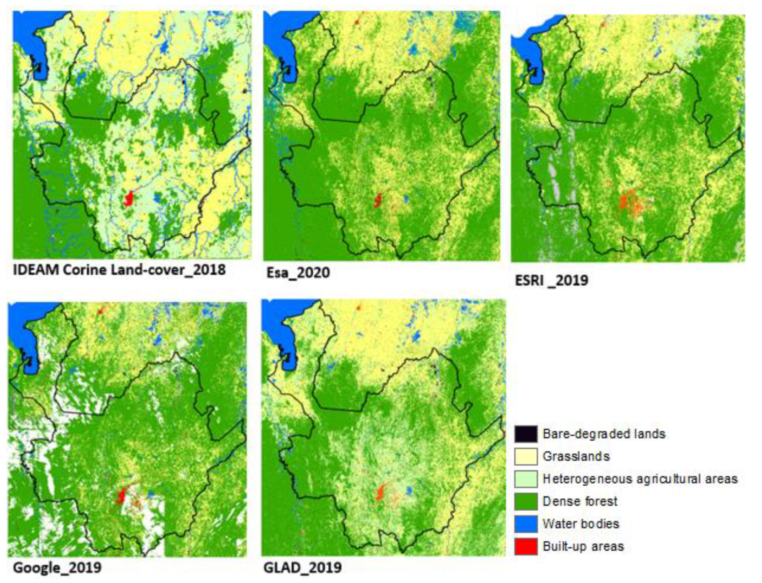
| Product | Accuracy | F1_Score |
|---|---|---|
| Google_2019 | 0.56 | 0.56 |
| Esri_2019 | 0.59 | 0.56 |
| Esa_2020 | 0.61 | 0.60 |
| Glad_2019 | 0.69 | 0.67 |
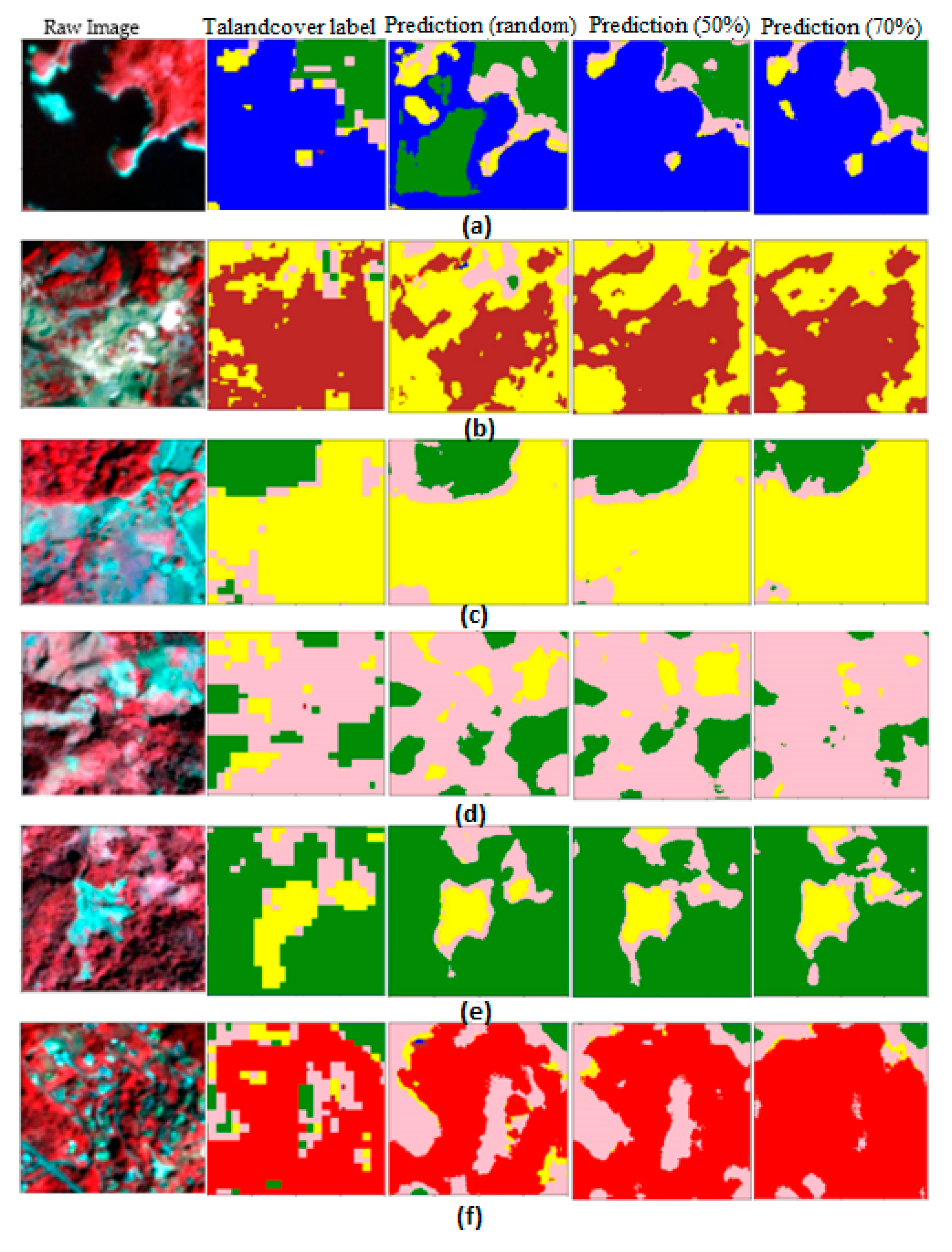
| Talandcover map | 0.75 | 0.76 |
| Coverage Type | 50% | 70% |
|---|---|---|
| Bare-degraded lands | 234 | 122 |
| Grasslands | 22,515 | 10,228 |
| Heterogeneous agricultural areas | 26,225 | 7414 |
| Dense forest | 61,610 | 45,617 |
| Bodies of water | 670 | 343 |
| Built-up areas | 1004 | 689 |
| Training | 1111 | 584 |
| Test | 278 | 147 |
| Total | 1389 | 731 |
| Random Sample | 50% Sample | 70% Sample | |||||
|---|---|---|---|---|---|---|---|
| Class | Training | Test | Training | Test | Training | Test | |
| Bare-degraded lands | px | 345,589 | 67,380 | 1,815,872 | 700,986 | 1,228,192 | 308,143 |
| % | 0.53% | 0.41% | 9.98% | 15.39% | 12.84% | 12.79% | |
| Grasslands | px | 14,648,492 | 3,825,272 | 4,300,293 | 1,135,534 | 2,049,492 | 484,262 |
| % | 22.35% | 23.35% | 23.62% | 24.93% | 21.42% | 20.11% | |
| Heterogeneous agricultural areas | px | 15,655,124 | 3,831,559 | 3,751,735 | 842,770 | 1,819,210 | 419,836 |
| % | 23.89% | 23.39% | 20.61% | 18.50% | 19.01% | 17.43% | |
| Dense forest | px | 33,541,637 | 8,318,905 | 4,055,664 | 883,921 | 1,794,289 | 525,788 |
| % | 51.18% | 50.77% | 22.28% | 19.41% | 18.75% | 21.83% | |
| Bodies of water | px | 264,911 | 105,181 | 1,988,487 | 545,079 | 1,293,598 | 332,603 |
| % | 0.40% | 0.64% | 10.92% | 11.97% | 13.52% | 13.81% | |
| Built-up areas | px | 1,080,247 | 235,703 | 2,290,573 | 446,462 | 1,383,475 | 337,816 |
| % | 1.65% | 1.44% | 12.58% | 9.80% | 14.46% | 14.03% | |
| Parameter | Value |
|---|---|
| Input Channels | NIR (Near-Infrared), R (Red), G (Green) |
| Epochs | 60 |
| Batch Size | 16 |
| Optimization Function | Adam (Adaptive Moment Optimization) |
| Beta_1 | 0.9 |
| Beta_2 | 0.999 |
| Epsilon | 1 × 10⁻⁷ |
| Loss Function | Sparse Categorical Cross Entropy |
| Learning Rate | 0.001 |
| Regularization Method | Dropout rate 0.5 |
| Item | Description |
|---|---|
| Application field | Satellite image segmentation |
| Type of Data collected | NICFI satellite images: planet_medres_normalized_analytic_2018-12_2019-05_mosaic |
| GIS Software Used | QGIS 1 V3.22.2 |
| Scripting Language for Data Processing and Products | Python 3.8 |
| Packages Used in Programming Language | GDAL2, OGR 3 |
| Collection Year | 2019 |
| Number of Classes | 6 |
| Type of Segmented Data | Multiclass mask |
| Dataset Size | 747.8 MB (.zip) |
| Image Format | Tif |
| Number of Images | 1389 (balanced-50%)-731 (balanced-70%)-5000 (random) |
| Rows and Columns | 128 × 128 |
| Spectral Resolution of Images | 4 bands, R-G-B-NIR |
| Radiometric Resolution of Images | 16 bit |
Disclaimer/Publisher’s Note: The statements, opinions and data contained in all publications are solely those of the individual author(s) and contributor(s) and not of MDPI and/or the editor(s). MDPI and/or the editor(s) disclaim responsibility for any injury to people or property resulting from any ideas, methods, instructions or products referred to in the content. |
© 2023 by the authors. Licensee MDPI, Basel, Switzerland. This article is an open access article distributed under the terms and conditions of the Creative Commons Attribution (CC BY) license (https://creativecommons.org/licenses/by/4.0/).
Share and Cite
Gomez-Ossa, L.F.; Sanchez-Torres, G.; Branch-Bedoya, J.W. Land Cover Classification in the Antioquia Region of the Tropical Andes Using NICFI Satellite Data Program Imagery and Semantic Segmentation Techniques. Data 2023, 8, 185. https://doi.org/10.3390/data8120185
Gomez-Ossa LF, Sanchez-Torres G, Branch-Bedoya JW. Land Cover Classification in the Antioquia Region of the Tropical Andes Using NICFI Satellite Data Program Imagery and Semantic Segmentation Techniques. Data. 2023; 8(12):185. https://doi.org/10.3390/data8120185
Chicago/Turabian StyleGomez-Ossa, Luisa F., German Sanchez-Torres, and John W. Branch-Bedoya. 2023. "Land Cover Classification in the Antioquia Region of the Tropical Andes Using NICFI Satellite Data Program Imagery and Semantic Segmentation Techniques" Data 8, no. 12: 185. https://doi.org/10.3390/data8120185