LoRaWAN Path Loss Measurements in an Urban Scenario including Environmental Effects

Abstract

LoRaWAN is a widespread protocol by which Internet of things end nodes (ENs) can exchange information over long distances via their gateways. To deploy the ENs, it is mandatory to perform a link budget analysis, which allows for determining adequate radio parameters like path loss (PL). Thus, designers use PL models developed based on theoretical approaches or empirical data. Some previous measurement campaigns have been performed to characterize this phenomenon, primarily based on distance and frequency. However, previous works have shown that weather variations also impact PL, so using the conventional approaches and available datasets without capturing important environmental effects can lead to inaccurate predictions. Therefore, this paper delivers a data descriptor that includes a set of LoRaWAN measurements performed in Medellín, Colombia, including PL, distance, frequency, temperature, relative humidity, barometric pressure, particulate matter, and energy, among other things. This dataset can be used by designers who need to fit highly accurate PL models. As an example of the dataset usage, we provide some model fittings including log-distance, and multiple linear regression models with environmental effects. This analysis shows that including such variables improves path loss predictions with an RMSE of 1.84 dB and an R² of 0.917.

Dataset:https://github.com/magonzalezudem/MDPI_LoRaWAN_Dataset_With_Environmental_Variables

Dataset License: CC-BY 4.0

1. Introduction

The Internet of things (IoT) is an enabling paradigm of Industry 4.0 that uses sensors to extract environment-aware data in diverse applications, such as domotics [1], smart energy [2], and precision agriculture [3], among other things. The data collected is further stored and analyzed to perform classifications or regressions, helping organizations make decisions about their processes [4]. Although there are applications where the end nodes (ENs) transmit information over short distances and have unlimited energy resources (e.g., domotics), there are also some cases where the ENs must be deployed in hard-to-access places where the sensors’ information has to be transmitted over distances, and where changing batteries is difficult or impossible, e.g., in forest fire monitoring [5], regulating the water level in dams [6], and landslide detection [7]. Thus, when the application has low energy and long-distance constraints, low power wide area networks (LPWANs) are used because they exhibit a good compromise between range and power consumption [8]. One of the most widespread protocols for LPWANs is LoRaWAN [9], which has gained popularity for IoT deployments because it operates in unlicensed bands, consumes low energy, and covers wide ranges compared to other competitors like narrow-band IoT (NB-IoT) or Sigfox [10].

Because LoRaWAN is a wireless sensor network (WSN) protocol [11], deploying ENs in the field requires previous network planning and link budget analyses. These analyses help establish the network parameters that achieve reliable connectivity at low energy consumption, so designers can choose different radio elements, including antennas’ geometries, antennas’ gains, allowed attenuations caused by cables and connectors, expected path loss (PL) and shadowing features posed by the channel, and transmission powers [12]. Consequently, the link budget calculation guarantees that the received signal strength indicator (RSSI) on the gateway (GW) side is sufficiently large to be demodulated correctly. The PL effects can be estimated by using theoretical models (e.g., Friis [13], and two-ray [12]) or empirical models (e.g., Okumura–Hata [14] and log-distance models [12]) to accomplish the link margin goals. More specifically, the Friis approach considers that the PL depends only on distance and frequency and does not consider multipath phenomena that cause shadowing [15]. Besides, the two-ray model considers a theoretical approximation of the line of sight (LoS) ray and the ray reflected over the ground, so it partially considers shadow fading effects [12].

However, because the multipath phenomenon in real applications is very diverse and complex, empirical models based on measurement campaigns are also proposed. For instance, the Okumura–Hata approach [14] provides a closed-form expression derived from collected data in Tokyo, Japan. It depends on the distance between the EN and the GW, the antenna heights, and the frequency. This model was fitted for large cells where the antennas’ heights are from 30 to 100 $\mathrm{m}$; however, in WSN/IoT networks, ENs’ antennas are close to the ground (for example, in precision agriculture [16]), causing shadow fading effects up to 14 dB [12], which may not be suitable for IoT applications, considering that the maximum transmitter power is about 20 dBm (e.g., LoRaWAN [9]). Because of these limitations, a log-distance path loss model (LDPLM) is also fitted from field data, including a shadow fading term, which is modeled considering that the probability density function (PDF) attends a lognormal distribution. In that way, according to [17], the statistical validity of the LDPLM must meet the following conditions: (i) pass an analysis of variance (ANOVA) test, by which the log-distance weight (also known as a path-loss exponent) is analyzed to check its significance, and (ii) the residual error/shadow fading term must be log-normally distributed, homoscedastic, and uncorrelated. However, in the proposed models, these tests are rarely addressed, and in the cases where it is handled, normality is not always met ([18,19]).

Due to the limitations mentioned above, some previous datasets have tackled the problem of modeling the radio frequency features in LoRaWAN networks to improve PL predictions. For instance, in [20], the authors collected 665 samples in the city of Beirut, Lebanon, logging timestamp, distance, frequency (868 MHz), RSSI, signal-to-noise ratio (SNR), GW coordinates, and spreading factor (SF), with a fixed bandwidth (BW) of 125 kHz and a fixed payload of 37 bytes. An LDPLM was enhanced by adding a new feature based on the EN antenna height. After fitting the corresponding model, they found a PL standard deviation of 7.2 dB.

Another approach can be found in [21], wherein the authors collected some operational aspects of LoRaWAN in Brno, Czech Republic. Regarding PL modelling, the authors collected data for two months, logging timestamp, RSSI, SNR, timestamp, GW coordinates, EN coordinates, time on air (ToA), frequency (868 MHz), SF, payload size, and frame count. They found that the RSSI fluctuated up to 50 dB, concluding that the conventional propagation models may lead to significant inaccuracies in PL prediction.

Furthermore, in [22], the authors deployed nine GWs in central London, UK, and collected timestamp, frequency (868 MHz), RSSI, SNR, SF, and payload size. However, this dataset does not include the distance between the GW and the ENs, so its use is mainly oriented to optimizing network parameters, and PL modelling is impossible.

Moreover, in [23], the authors provide a dataset for localization/tracking purposes by using fingerprinting techniques by which the base station position is not needed. This dataset provides the RSSI of 68 base stations, timestamp, SF, and EN coordinates, for three months, in the city center of Antwerp, Belgium. As an application, this approach shows a fingerprint location using clustering techniques, particularly KNN [24], achieving a mean error of $398.4$ $\mathrm{m}$. In that way, this dataset is unsuitable for PL modelling purposes.

In addition, because our dataset can be mainly used for path loss modeling, we retrieved the most recent approaches for LoRaWAN to further exhibit our dataset’s contribution. For instance, Anzum et al. [25] proposed a LoRaWAN path loss model to characterize the attenuation in oil palm crops by using an LDPLM mainly based on the distance between the ENs and the GW and the number of canopies and trunks throughout the communication path. Alobaidy et al. [26] fitted a semiempirical machine-learning-based path loss model for LoRaWAN links combining the Friis model with a stepwise multiple linear regression that depends on the frequency, bandwidth, antennas’ heights, spreading factor, and distance. Batalha et al. [27] performed a measurement campaign by using LoRaWAN in a suburban environment and fitted close-in and floating intercept LDPLMs that depend on the distance between the ENs and the GW; then, they compared their performance versus the Okumura–Hata model. Bianco et al. collected path loss measurements in a mountain environment, fitted an LDPLM by using the distance as a predictor variable, and used it in tracking and rescue applications. Callebaut et al. [28] evaluated coverage and path loss in urban, forest, and coastal environments and fitted a two-slope LDPLM to assess the protocol’s reliability in each scenario. Finally, El Chall et al. [20] proposed different LDPLMs for indoor, campus, and city environments. The contributions regarding datasets and path loss models are summarized in

Table 1. LoRaWAN path loss models.

Reference	Description	Variables	Model Type
Aernouts et al. [23]	Measurement campaign to evaluate fingerprinting algorithms for LoRaWAN and Sigfox	RSSI, timestamp, location	Not reported
Anzum et al. [25]	Path loss model to characterize the attenuation in oil palm crops	Distance, number of trees and canopies	LDPLM
Alobaidy et al. [26]	Path loss model to improve the reliability of transmission in a water quality monitoring application	Distance, frequency, bandwidth, antennas’ heights, and spreading factor	ML-based
Batalha et al. [27]	Path loss model for suburban environments to analyze the impacts of path loss in coverage, SNR, and received packets	Distance	LDPLM
Bhatia et al. [22]	LoRaWAN campaign collected from nine GWs over four months in an urban environment	RSSI, SNR, and SF	Not reported
Bianco et al. [29]	Path loss model to improve the localization in search and rescue application, particularly for mountain environments	Distance	LDPLM
Callebaut et al. [28]	Path loss model for different environments, such as urban, forests, and coasts	Distance	LDPLM
El Chall et al. [20]	Path loss model for indoors, campus, city, and suburban environments	Distance	LDPLM
Masek et al. [21]	LoRaWAN dataset of operational aspects in campus and urban environments in Czech Republic	Distance, frequency, RSSI, SNR, SF, GW location, EN location, PL	LDPLM

.

As presented in Table 1, the measurement campaigns and path loss models for LoRaWAN are mainly based on distance, frequency, and antennas’ heights. However, previous studies have shown that PL variability is also accentuated by the change of some environmental-related variables like temperature [30], relative humidity [31], barometric pressure ([32]), and particulate matter [33]. However, these effects have not been measured in the available LoRaWAN datasets. In that way, this paper provides a comprehensive LoRaWAN measurement campaign carried out in an urban environment, in Medellín, Colombia, for four months. Our measurement setup includes one GW, and four fixed ENs from 2 $\mathrm{k}$$\mathrm{m}$ to 8 $\mathrm{k}$$\mathrm{m}$. The dataset has up to 930.000 observations, including geometric conditions (distance and antennas’ heights), link budget features (transmitter powers, antennas’ gains, cables and connectors attenuations, carrier frequency, SF, and frame length), propagation variables (RSSI, SNR, ToA, effective signal power (ESP), noise power (P_n), and consumed energy) and environmental variables (temperature, relative humidity, barometric pressure, and particulate matter). The main contribution of building this dataset is the inclusion of the environmental variables because designers can fit more accurate path loss and shadowing models depending on weather variations.

The rest of this paper is organized as follows. Section 2 briefly introduces the main features of the LoRaWAN protocol. Section 3 specifies the logged fields in the dataset. Section 4 shows the experimental setup from the ENs’ construction to the database logging. Section 5 shows a possible application of PL modelling using the dataset, including a lognormal combined path loss and shadowing (CPLS) model and an environment-based CPLS model that improves the prediction errors and increases the correlation factor. Finally, Section 6 shows the conclusions.

2. LoRaWAN Outline

This section provides a brief description of the LoRaWAN protocol. It includes the architecture, spectrum utilization, modulation characteristics, and transmission power control (TPC) strategies.

2.1. Architecture

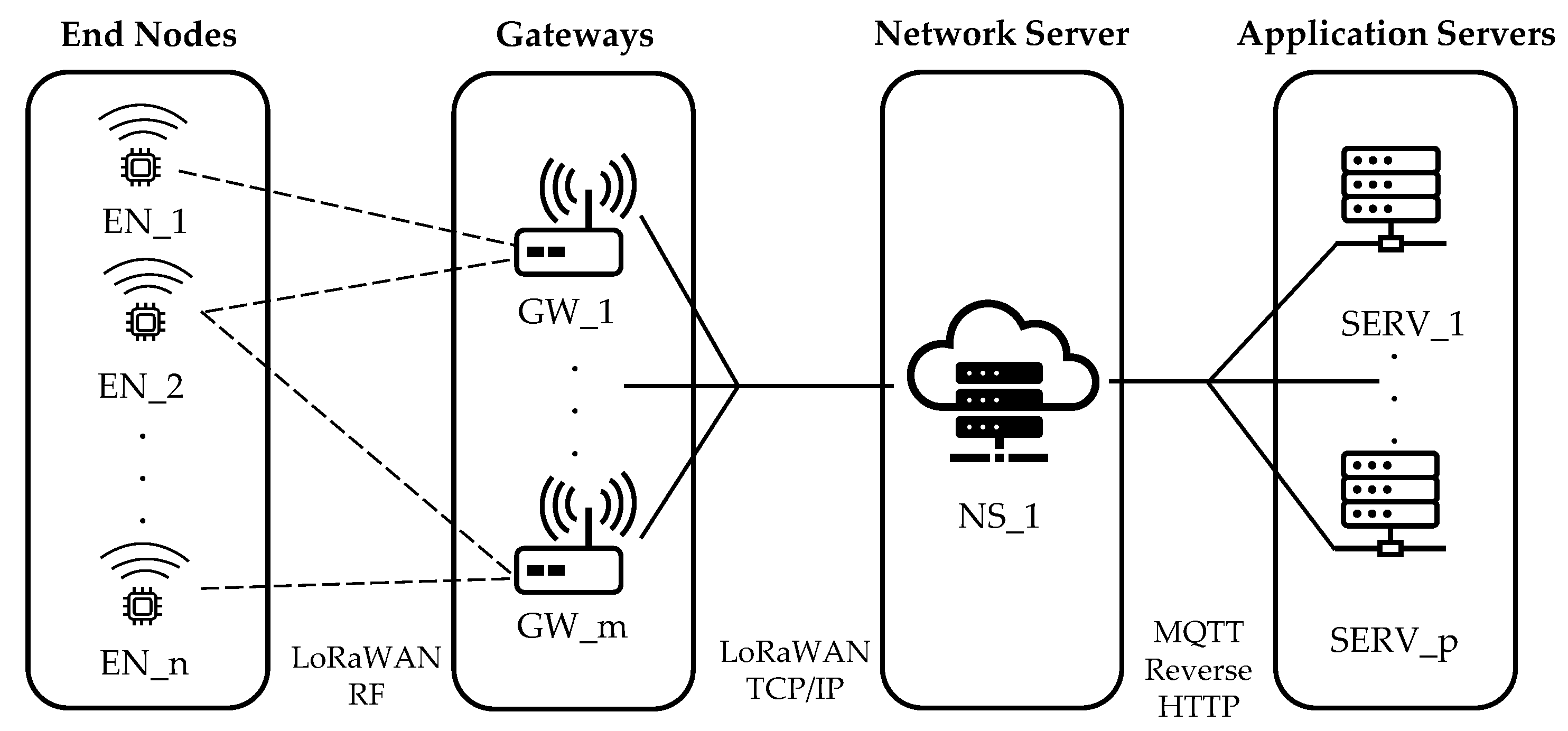
The network architecture of LoRaWAN [9] is depicted in Figure 1. It includes four entities: (i) the ENs, which are in charge of sensing variables, and transmit them via LoRaWAN radio frequency (RF) protocol, (ii) the GWs, which receives the information from the ENs and retransmit it to a server via LoRaWAN TCP/IP, (iii) the network server (NS) that receives the information from the GWs, deletes duplicates, and exhibits some services to send information to the applications by using different protocols like message queue telemetry transport (MQTT) or reverse hypertext transport protocol (Reverse HTTP), and (iv) application servers that receive information from the NS and store it, analyze it, or visualize it. Mainly, if an EN needs to transmit a frame, it sends a broadcast message that various GWs can receive. In this case, the same frame can be retransmitted by more than one GW, so the NS filters the information and puts the information into an MQTT broker or a cloud-based server.

2.2. Spectrum Usage

LoRaWAN operates in the industrial, scientific, and medical (ISM) bands, which are unlicensed in most countries, so users do not have to pay any fee for their utilization [34]. In the case of Europe, the accepted frequency ranges are from 863 $\mathrm{M}$$\mathrm{Hz}$ to 870 $\mathrm{M}$$\mathrm{Hz}$, divided into 16 upload/download channels of BW equal to 125 $\mathrm{k}$$\mathrm{Hz}$. In the case of America, the accepted frequency ranges are from 902 $\mathrm{M}$$\mathrm{Hz}$ to 928 $\mathrm{M}$$\mathrm{Hz}$, divided into 64 uplink channels of BW of 125 $\mathrm{k}$$\mathrm{Hz}$, eight uplink channels of BW of 500 $\mathrm{k}$$\mathrm{Hz}$, and eight downlink channels of a BW of 500 $\mathrm{k}$$\mathrm{Hz}$. Our dataset was generated in the approved band for America (US902-928). Because the ISM bands are intensively used, designers must attend duty cycle policies that demand to wait a period until a new transmission. For instance, in Europe, the duty cycles must be under 1%, and in America, there are no duty cycle limitations, but a transmission must not last more than 400 ms.

2.3. Modulation

LoRaWAN uses chirp spread spectrum (CSS) for modulation [35]. This spread spectrum technique helps reduce interference and multipath and fading effects [23]. If the central carrier frequency is $f_0$, a chirp signal changes its frequency linearly in the interval ($f_0-$$BW$/2, $f_0$ + $BW$/2) during a symbol time $T_s$. In addition, the channel bandwidth is divided according to the SF parameter (i.e., the number of bits per symbol), which takes values from 6 to 12. Thus, the spectrum is divided into $2^{SF}$ parts so that the symbols can start at $2^{SF}$ at different initial frequencies. The initial frequency determines the value to be transmitted, so any symbol can carry up to $2^{SF}$ values. Furthermore, a coding rate (CR) parameter defines the proportion of redundancy bits added to the frame for error correction and can take values of 4/5, 4/6, 4/7, and 4/8. The symbol time $T_s$ can be defined in Equation (1):

$$T_s={\displaystyle \frac{2^{SF}}{BW}}.$$

(1)

It can be noticed that increasing the SF by one multiplies per two the symbol time $T_s$. In addition, the SF modifies the receiver sensitivity allowing negative SNR limit values, as shown in

Table 2. SNR limit versus spreading factor dependency [36].

Spreading Factor	SNR Limit (dB)
7	−7.5
8	−10
9	−12.5
10	−15
11	−17.5
12	−20

. In this way, changing SF allows broader coverage but increases $T_s$. Because the consumed energy depends on the transmission power and $T_s$, increasing this parameter means the energy will also increase.

2.4. Transmission Power Control

LoRaWAN includes an adaptative data rate (ADR) algorithm as a TPC scheme, which is used to improve energy consumption dynamically. The idea behind this scheme is to change the transmission parameters (transmission power and SF) according to the channel state, particularly the behavior of the SNR. As previously discussed, when the SF increases, the effect is that the SNR${}_{limit}$ can be worse [36], as shown in Table 2. The SNR${}_{limit}$ is the worst SNR the receiver can tolerate to demodulate the received signal adequately. In the case of LoRaWAN, the SNR${}_{limit}$ can be negative; that is, the received signal power can be less than the noise floor power. The steps to implement the ADR algorithm are discussed as follows [37].

• The EN enables the ADR scheme and informs the GW. Hence, the NS can change the transmission power and the SF. In addition, the EN sends information with an SF = 12 to guarantee that the data can reach the gateway.
• The base station collects 20 values of SNR (SNR${}_{measured}$) from the node and sends them to the network server.
• The network server takes the maximum value of the 20 SNR${}_{measured}$ samples, for example, 5 dB. It also takes the current SF.
• The network server calculates the margin $M_e$ as shown in Equation (2),

  $$M_e=SN{R}_{measured}-SN{R}_{limit}-LM,$$

  (2)

  where $LM$ is the link margin, used as a security term to achieve reliable communications. For example, $LM$ = 10, SNR${}_{limit}$ = $-20$ dB (SF = 12, from Table 2), so $M_e$ = 5 dB − (−20 dB) −10 dB = 15 dB. It means an excess of 15 dB in the link budget, which causes a waste of energy.
• The network server calculates the $M_e$ again with a lower spreading factor (it always must be greater than zero to guarantee a stable link). For example, for SF = 7, $SN{R}_{limit}$ = $-7.5$ dB, so $M_e$ = 5 dB − (−7.5 dB) − 10 dB = 2.5 dB.
• Because there is an excess of 2.5 dB, the network server also lowers the transmission power.

3. Data Description

The given dataset contains a comma-separated values file with the measurements of four ENs and one GW in Medellín, Colombia. The database includes 930,753 observations from October 2021 to March 2022, with a mean sample time of 60 s. According to the regulations of the ISM bands for US915, the maximum transmission time is 400 ms [38]. In that way, we transmitted up to 242 bytes with SF = 7, 125 bytes with SF = 8, 53 bytes with SF = 9, and 11 bytes with SF = 10. These frame sizes and SFs guarantee that the transmission time is less than 400 ms (https://www.thethingsnetwork.org/airtime-calculator, accessed on 14 December 2020) Furthermore, because each node transmitted data each 60 $\mathrm{s}$ and the maximum transmission time was 400 $\mathrm{m}$$\mathrm{s}$, we obtained that a duty cycle of $\frac{0.4}{60.4}\ast 100=0.662\%$, which is recommended to have a fair use of the spectrum (obtained with SF = 7 and frame size of 242 bytes).

The fields in the dataset are described as follows.

• index: Sequential number that identifies the corresponding observation.
• timestamp: Date and time mark of the current observation. It is in format yyyy-mm-dd hh:mm:ss.
• device_id: String that identifies the EN’s name of the current measurement. The corresponding names can be EN1, EN2, EN4, and EN4.
• distance: Distance between the GW and the corresponding EN, in meters.
• ht: Antenna height of the corresponding EN, in meters.
• hr: Antenna height of the GW, in meters. Because the GW was installed in a static position, this height is fixed.
• ptx: Transmitter (EN) radiated power in dBm. It was fixed to 20 dBm.
• ltx: Transmitter (EN) losses associated with cables and connectors, in dB.
• gtx: Transmitter (EN) antenna gain (characterized with a vector network analyzer), in dBi.
• lrx: Receiver (GW) losses associated with cables and connectors, in dB. The measured attenuation was 4.25 dB.
• grx: Receiver (GW) antenna gain (characterized with a vector network analyzer), in dBi. The measured gain was 4.161 dBi.
• frequency: Carrier frequency, in $\mathrm{Hz}$. The experiments were performed in the US902-928 ISM band.
• frame_length: Number of bytes of the current transmission’s payload.
• temperature: Temperature of the environment, in °C.
• rh: Relative humidity of the environment, in %.
• bp: Barometric pressure of the environment, in hPa.
• pm2_5: Particulate matter PM2.5 of the environment, in $\mathsf{\mu }$g/m³.
• rssi: Received signal strength indicator at the GW, in dBm.
• snr: Signal-to-noise ratio in dB.
• toa: Time on air, in seconds.
• experimental_pl: Experimental path loss (in dB) calculated by $ptx+gtx+grx-lrx-rssi$.
• energy: Consumed energy of the current transmission, in Joules.
• esp: Effective signal power of the current transmission, in dBm.
• pn: Noise power, in dBm.

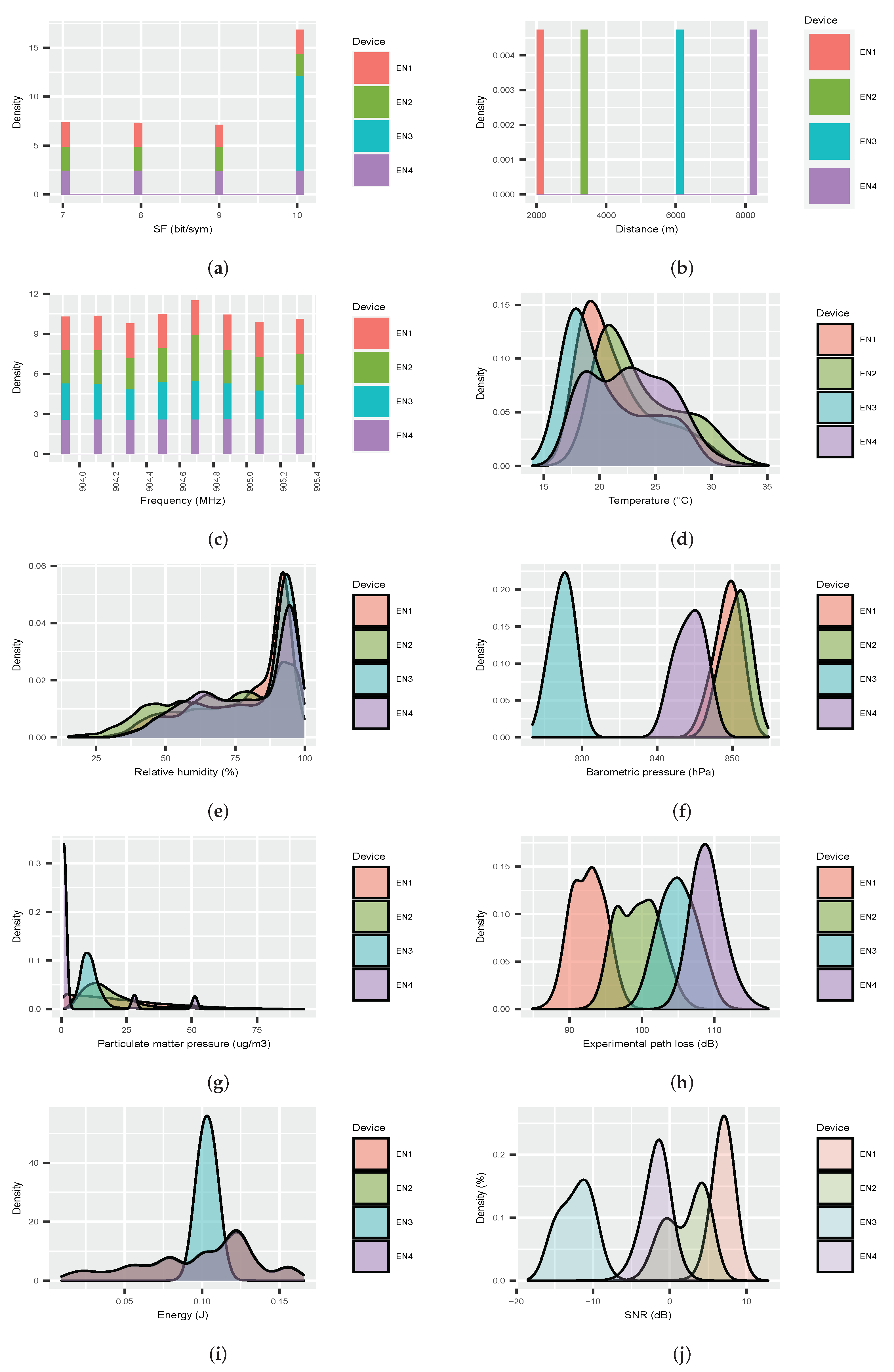
A statistical description of the numerical dataset fields is shown in

Table 3. Statistical description of the dataset fields.

Variable	Unit	Min	1st Quartile	Median	Mean	3rd Quartile	Max
distance	m	2140	3450	6100	5107	6100	8260
ht	$\mathrm{m}$	8	8	12	16.67	12.5	40
hr	$\mathrm{m}$	5	5	5	5	5	5
ptx	m	20	20	20	20	20	20
ltx		1	1	1	4.824	11.75	11.75
gtx	i	2.903	2.923	2.923	4.094	2.995	8.536
lrx		4.25	4.25	4.25	4.25	4.25	4.25
grx	i	4.161	4.161	4.161	4.161	4.161	4.161
frequency	$\mathrm{M}$$\mathrm{Hz}$	903.9	904.1	904.7	904.59	904.9	905.3
sf	bit/sym	7	8	10	9	10	10
frame_length	byte	9	9	10	39.91	53	241
temperature	°C	13.9	18.8	21.1	21.91	24.7	35.1
rh	%	1	64.1	84.5	77.87	93.2	99.8
bp	hPa	822.8	828.4	845.1	840.5	849.5	854.8
pm2_5	$\mathsf{\mu }$g/m3	0	3	6	10.01	15	93
rssi	m	−105	−93	−82	−83.12	−75	−63
snr		−18.5	−11.5	−1.5	−3.064	4.8	12.8
toa	second	0.04122	0.2409	0.24781	0.2399	0.28877	0.379
exp_pl		84.91	96.81	103.81	102.2	107.08	117.4
energy	Joule	0.0093	0.0955	0.1038	0.09993	0.116	0.165

. In addition, the empirical distributions of the most representative variables are depicted in Figure 2. These descriptions help us understand how data is distributed. For instance, it can be noticed from Figure 2a that the SFs are uniformly distributed from 7 to 10 for ENs 1, 2, and 4; however, EN3 used only SF = 10 beause the distribution of the SNR exhibited a mean of −15 dB (Figure 2j), which means that SFs of 7 to 9 are not large enough to demodulate the received signals (Table 2). To guarantee uniform distribution of SF, we disabled the ADR scheme and controlled it manually. It also can be noticed that the carrier frequencies used are uniformly distributed overall (Figure 2c). Regarding the environmental variables, it can be noticed that the weather conditions describe tropical weather. For instance, temperatures were from 13.9 °C to 35.1 °C, and concentrated around 20 to 30 °C (Figure 2d). Furthermore, relative humidity was concentrated in high values, showing the common behavior in a tropical environment (Figure 2e). Moreover, particulate matter was concentrated in low values for EN4 because it is located inside a campus surrounded by a forest; however, there are two peaks in 28 and 50 $\mathsf{\mu }$g/m³, which are caused by a rock mine near the campus (Figure 2g). In addition, it can be noticed that the distribution of the experimental path loss is Gaussian-bell-shaped as expected [12] (Figure 2h). Finally, the distributions of consumed energy for ENs 1, 2, and 4 are similar; nevertheless, the EN3 has its energy concentrated around 0.1 J, which was caused by the fixed SF = 10 that guaranteed that the received signal could be demodulated.

Regarding the packet delivery rate (PDR) of each EN, we obtained 95.1%, 85.2%, 81.6%, and 86.35% for EN1, EN2, EN3, and EN4, correspondingly. These PDRs can be explained from the SNRs obtained for each EN, as depicted in Figure 2j. According to Table 2, varying the SF allows the signal power level to fall below the noise power level up to $-20$ dB. Furthermore, as we will see in Section 4.4, we distributed the SF uniformly for each EN from 7 to 10. In that way, we obtained PDRs according to the SNR of each EN. For instance, EN1 achieved SNRs over 0 dB, so getting a PDR of 95.1% is expected because many packages were delivered successfully. On the other hand, we notice that EN3 achieved the lowest PDR (81.6%) because the mean SNR is approximately $-15$ dB, so using a low SF can cause a loss of packets.

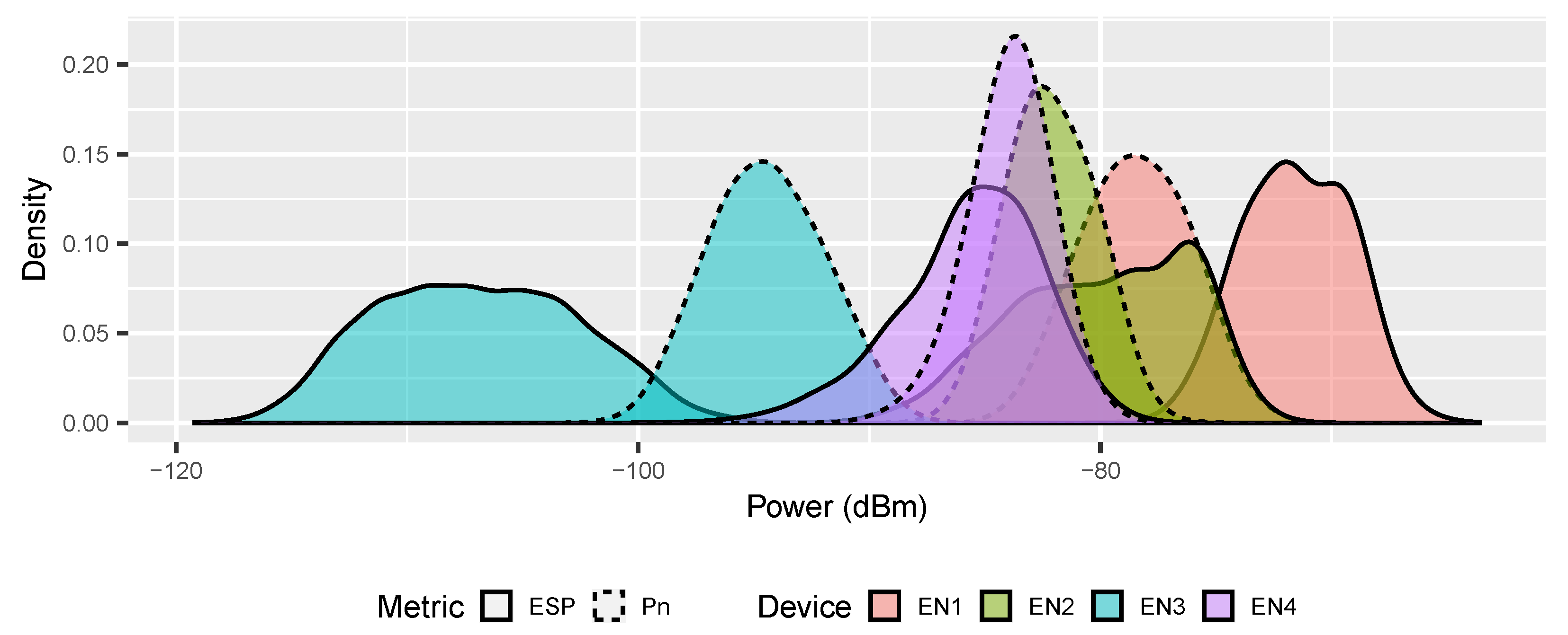
The dataset also includes the Effective Signal Power (ESP) metric, which is defined as the signal power in the receiver without including the noise power (Equation (3)) and the noise power $P_n$ (Equation (4)) [39]:

$$ES{P}_{\left(dB\right)}=RSS{I}_{\left(dB\right)}+SN{R}_{\left(dB\right)}-10·lo{g}_{10}(1+{10}^{\frac{SN{R}_{\left(dB\right)}}{10}})$$

(3)

$$P_{n\left(dB\right)}=RSS{I}_{\left(dB\right)}-10·lo{g}_{10}(1+{10}^{\frac{SN{R}_{\left(dB\right)}}{10}}).$$

(4)

The ESP and $P_n$ are relevant metrics by which to evaluate the quality of LoRaWAN radio links instead of RSSI and receiver sensitivity (traditionally, $RSSI>Sensitivity+LM$) because successful demodulation is achieved when $ES{P}_{\left(dB\right)}>P_{n\left(dB\right)}-SN{R}_{limit}+LM$. Thus, the ESP and $P_n$ empirical distributions are depicted in Figure 3, where it can be noticed that the ESP is always under the $P_n$, concluding that LoRaWAN can withstand very adverse channel conditions.

4. Experimental Setup

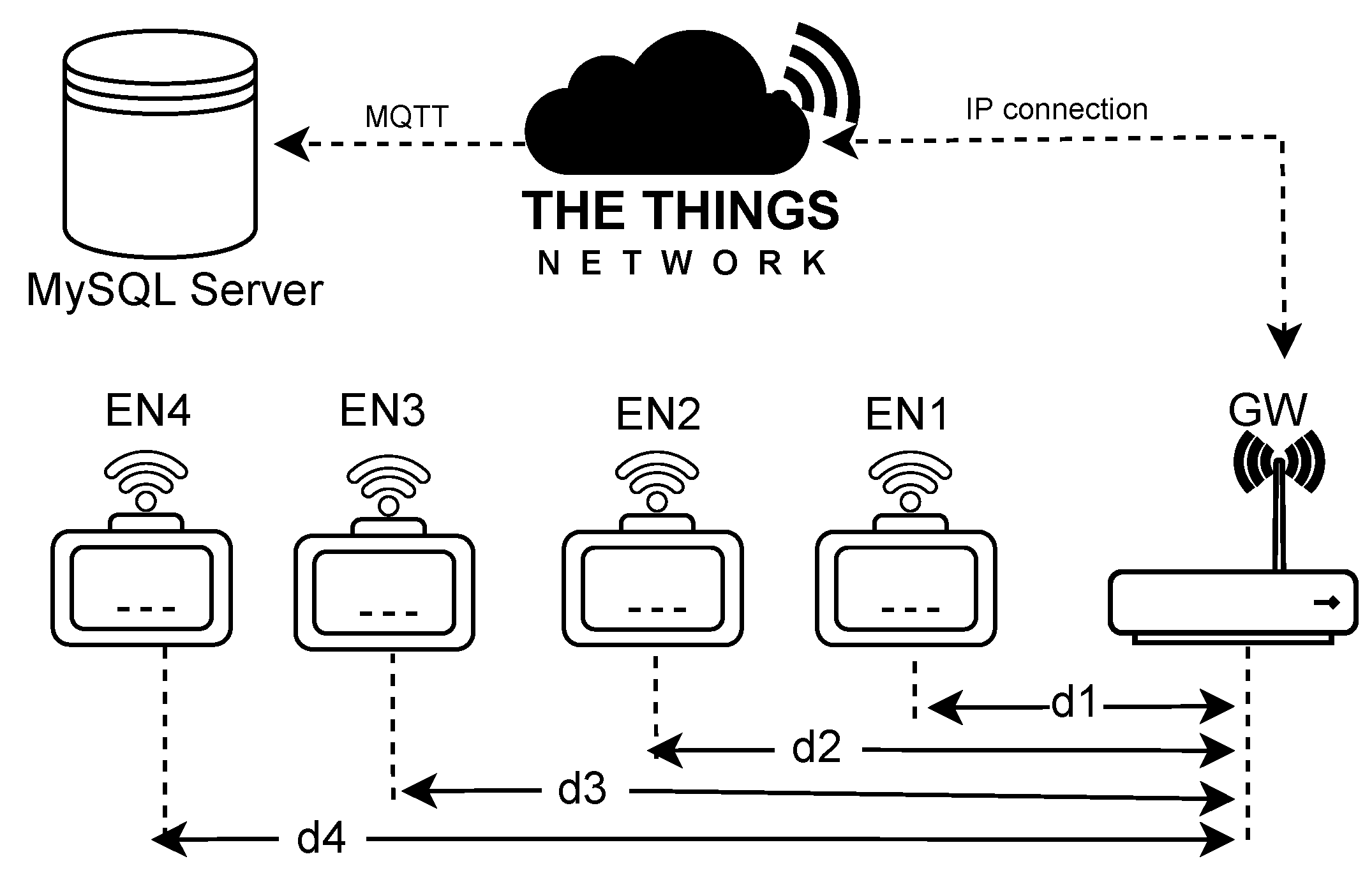
We have deployed a LoRaWAN setup to collect the variables included in this dataset. The system architecture follows the model previously explained in Figure 1. Mainly, we implemented the network shown in Figure 4. First, we deployed four ENs and one GW in different locations in the urban area of Medellín, Colombia, keeping LoS between each EN and the GW. Medellín is a medium-sized city with an area of 328 km² and about 4 million people. The city is located in the central part of the Andes Mountain Range, and its topography is a valley surrounded by mountains. The GW is connected to the Internet using an Ethernet connection. Once the GW receives a frame from an EN, it resends it to the selected NS. We used the things network (TTN), a widespread open-source NS. Because there are several LoRaWAN GWs in Medellín, we filtered the duplicated information in the NS to preserve only data from our GW. Subsequently, we enabled the MQTT broker provided by TTN and used a database cloud-based MySQL server to subscribe to the broker and get all the messages the NS receives. The following subsections describe each component deeply.

4.1. End Nodes

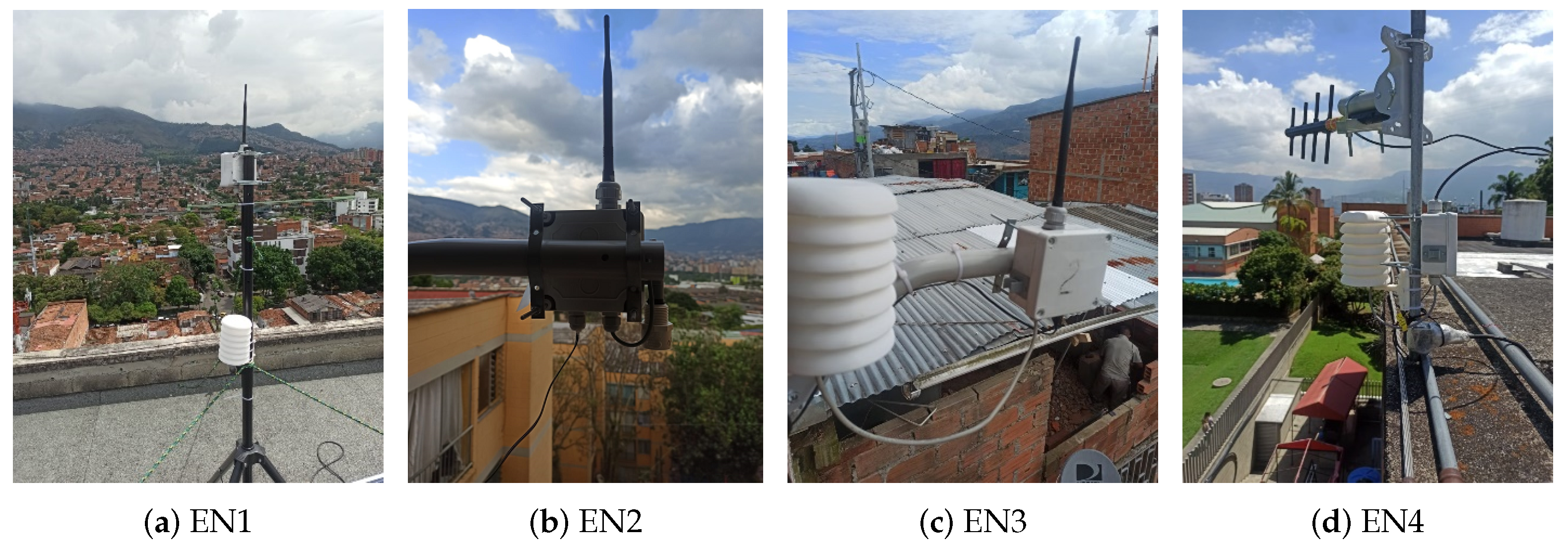
We selected the platform Pycom LoPy4 (https://pycom.io/product/lopy4/, accessed on 14 December 2022) to assemble and program the ENs because it meets processing and communications needs; hence, previous approaches use it [20]. The LoPy4 is a system-on-chip platform that embeds an Xtensa^® dual–core 32–bit LX6 microcontroller and four IoT radios, including LoRaWAN, Sigfox, Wi-Fi, and Bluetooth. Regarding LoRaWAN, the platform includes an SX1276 radio for ISM bands @ 433, 868, and 915 MHz. In addition, the processor can communicate with the environmental sensors by using different buses like serial peripheral interface (SPI), inter-integrated circuit (I2C), and universal asynchronous receiver and transmitter (UART). In addition, each EN has a transmission antenna. EN1, EN2, and EN3 use an omnidirectional antenna (Mobile Mark ref. PSKN3-900 (https://www.mobilemark.com/product/pskn3-900-1900s/, accessed on 14 December 2022)) with a peak gain of 3 dBi. Because these antennas are omnidirectional, their mounting angle was considered to be 90°. In addition, the EN4 uses a 4-elements Yagi–Uda antenna (Pulse Larsen ref. YA6900W (https://www.tessco.com/product/890-960mhz-8dbi-4-element-yagi-antenna-57677, accessed on 14 December 2022)) with a peak gain of 8.8 dBi, which was mounted such that the boom was parallel to the ground, with the directors perpendicular to the ground. Figure 5 depicts the antennas’ mounting positions.

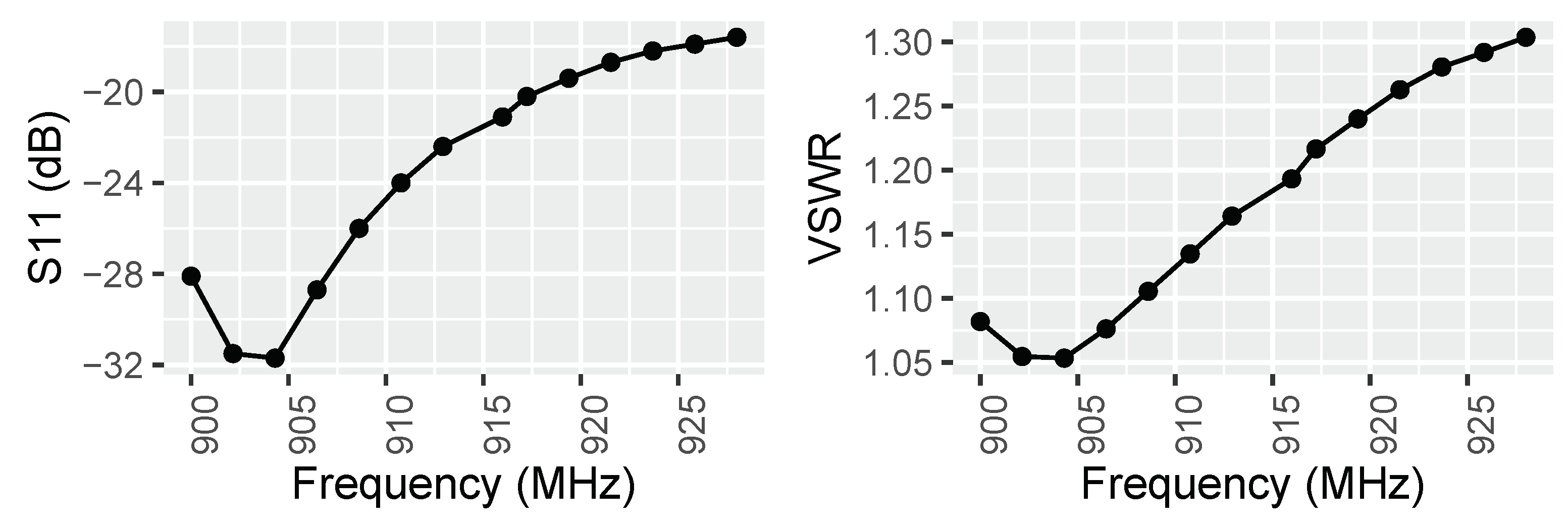
Furthermore, we performed an S11 and S21 analysis of the antennas and connectors by using a vector network analyzer (VNA). In particular, the S11 parameter delivers information on how much power is reflected from the antenna when a transmitter signal is supplied. In that way, this parameter allows designers to know how efficient the used antenna is. In addition, the S21 parameter measures how much power is transferred from port 1 to port 2 of the VNA, so it is used to determine attenuations/losses from cables and connectors. Carrying out these measurements guaranteed that the antenna gains and losses were accurate. An example of the S11 parametrization of our antennas is depicted in Figure 6.

4.2. Sensors

Each EN includes a set of sensors that captures weather variations. A brief description of each sensor is provided as follows.

• An Aosong DHT22 sensor for temperature (accuracy: ±0.5 °C) and relative humidity (accuracy: ±2%). Regarding temperature, this sensor includes a transistor-based transductor. Concerning relative humidity, it consists of a capacitive sensor. The sensor contains a one-wire communication protocol to send the current values to the LoPy4 microcontroller, lowering the errors in the analog-to-digital conversion.
• A Bosch BMP280 sensor for barometric pressure (accuracy: ±1 hPa). This sensor operates in a range of 300–1100 hPa, which is suitable for use in Medellín, Colombia because the barometric pressure is up to 900 hPa. This sensor embeds an I2C communication to communicate with the microcontroller, lowering the errors in analog-to-digital conversion.
• A Honeywell HPMA115S0 sensor for particulate matter PM2.5 (accuracy: ±15%). Its operation is based on laser scattering, which detects and counts particles with concentrations up to 1000 $\mathsf{\mu }$g/m³. The sensor communications are based on the RS232 protocol. Again, this communication reduces the errors in analog-to-digital conversion.
• In addition, we included a Texas Instruments INA219 energy sensor (accuracy ±0.5%) in the printed circuit board to quantify the consumption under different radio configurations. It is based on a shunt resistor that can monitor voltages up to 26 VDC and currents up to 5 A. The sensor sends the information to the microcontroller by using the I2C protocol.
• We added a Stevenson screen to protect the sensors from rainy conditions without losing accuracy and avoiding possible sensor saturations.

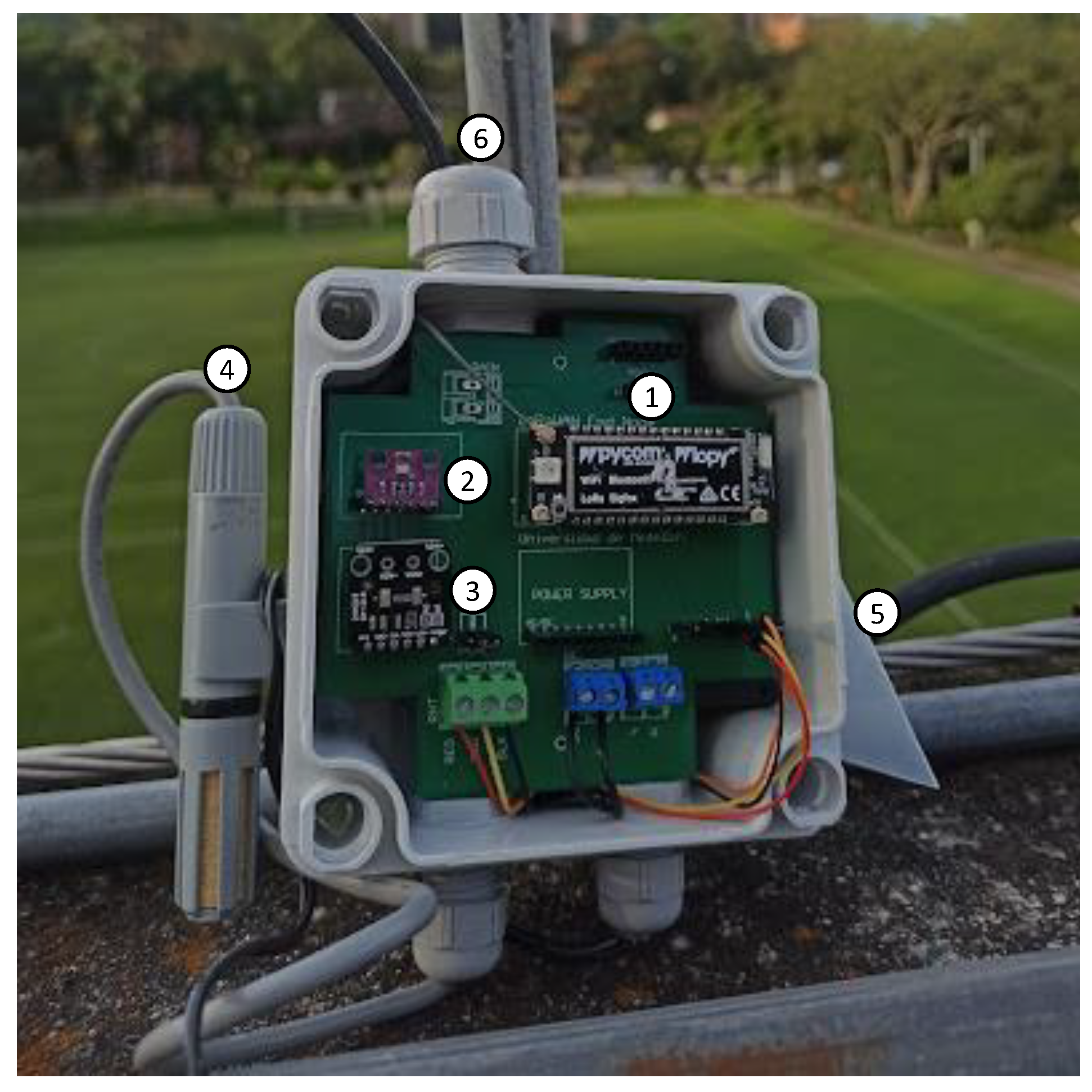
We also designed and built the ENs’ testbeds as shown in Figure 7. The electronics are inside a IP65 box to protect it from rain and condensation caused by high relative humidity.

4.3. Gateway

According to the architecture shown in Figure 4, the ENs must send the information to a GW that serves as a relay between the field data and the NS. Hence, we have selected, programmed, and deployed a GW Dragino LG308 (https://www.dragino.com/products/lora-lorawan-gateway/item/140-lg308.html, accessed on 14 December 2022) that incorporates two Semtech radios (SX 1257 and SX1301). Both radios can demodulate signals with a power greater than −140 dBm in 10 different channels simultaneously. Each radio uses a panel antenna (Wilson Electronics ref. 311155 (https://www.wilsonamplifiers.com/one-additional-panel-antenna-kit-for-db-pro-311155-k1/, accessed on 14 December 2022)) with a peak gain of 4.4 dBi. Furthermore, we checked the S11 parameter of each antenna to get an accurate experimental path loss. Finally, the GW receives the ENs’ frames via LoRaWAN radio frequency (RF) and resends them to the TTN via LoRaWAN IP.

4.4. Frame Configuration

Each EN packs the sensor’s information in a binary frame. To enlarge the corresponding scales, we multiply the measurements by 10 before sending them, and then, the NS divides by 10, preserving one decimal point as shown in

Table 4. Frame configuration sent from the ENs to the GW.

Variable	Max. Value	Max Value × 10	Binary Representation	# bits
Temperature	80 °C	800	1100100000	10
RH	100%	1000	1111101000	10
Barometric pressure	1000 hPa	10,000	10011100010000	14
PM2.5	400 $\mathsf{\mu }$g/m3	4000	111110100000	12
PM10	400 $\mathsf{\mu }$g/m3	4000	111110100000	12
Energy	65,535 Joule	65,535	1111111111111111	16
Total				74

, so the corresponding frame length is 74 bits. Moreover, we added some dummy bits to enlarge the frame length (six different sizes), so the dataset includes the effects of this parameter on energy consumption.

Furthermore, we used a BW of 125 $\mathrm{k}$$\mathrm{Hz}$ and iterated various subbands in the ISM US915 band (903.9, 904.1, 904.3, 904.5, 904.7, 904.9, 905.1, and 905 $\mathrm{M}$$\mathrm{Hz}$).

We also varied the SF with values of 7, 8, 9, and 10, according to the spectrum usage regulations. In summary, there are six frame configurations, eight subbands, and four SFs, so we transmit in 192 different radio configurations. Once the GW resends the information to TTN, the latter runs a payload formatter where the sensors’ readings are decoded, and the RSSI, ToA, and SNR are added to the final payload. Finally, TTN exposes an MQTT broker where the payloads are published, so we used a cloud-based server as an MQTT subscriber to get the messages and store them in a MySQL database.

4.5. Network Deployment

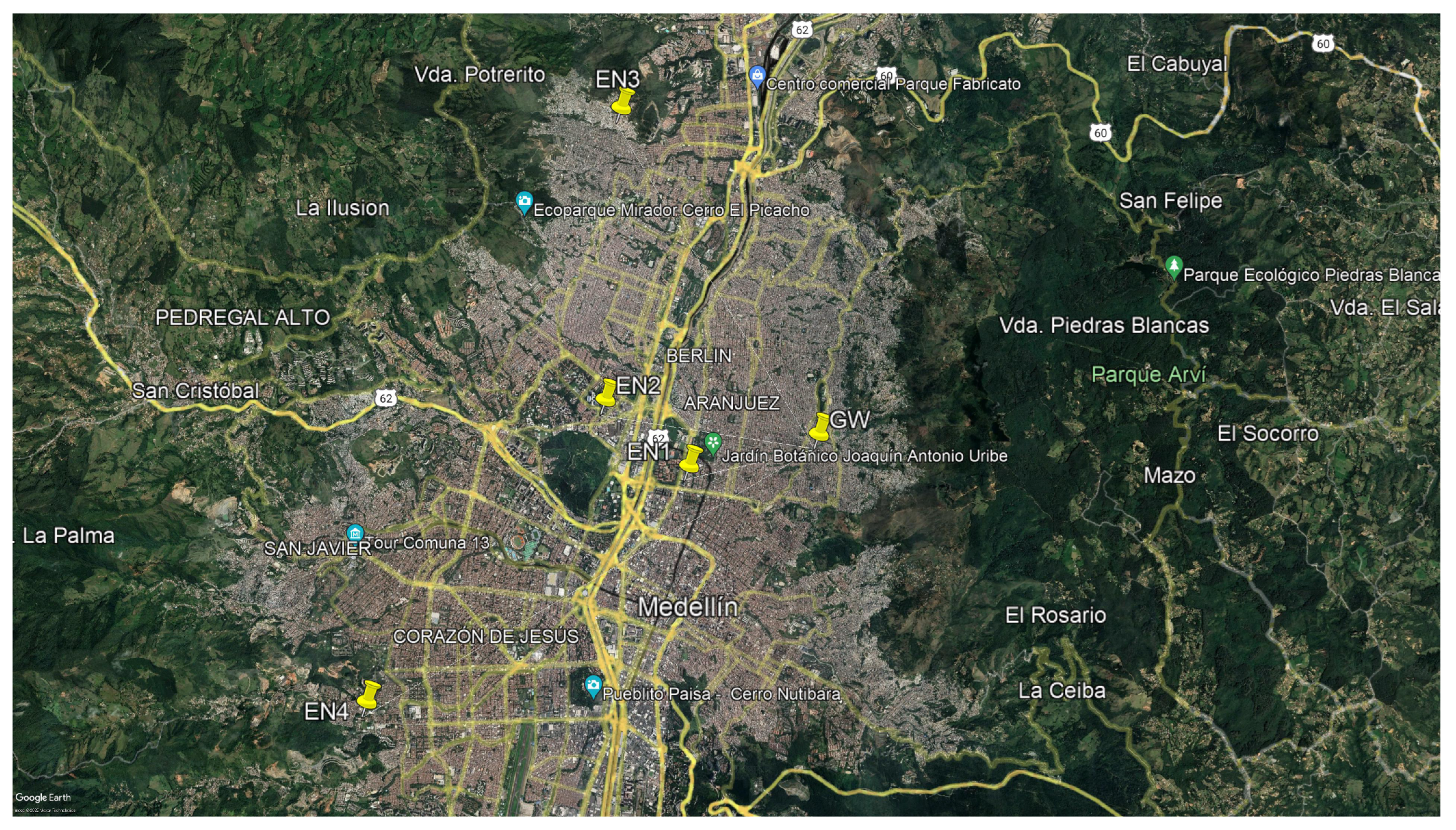
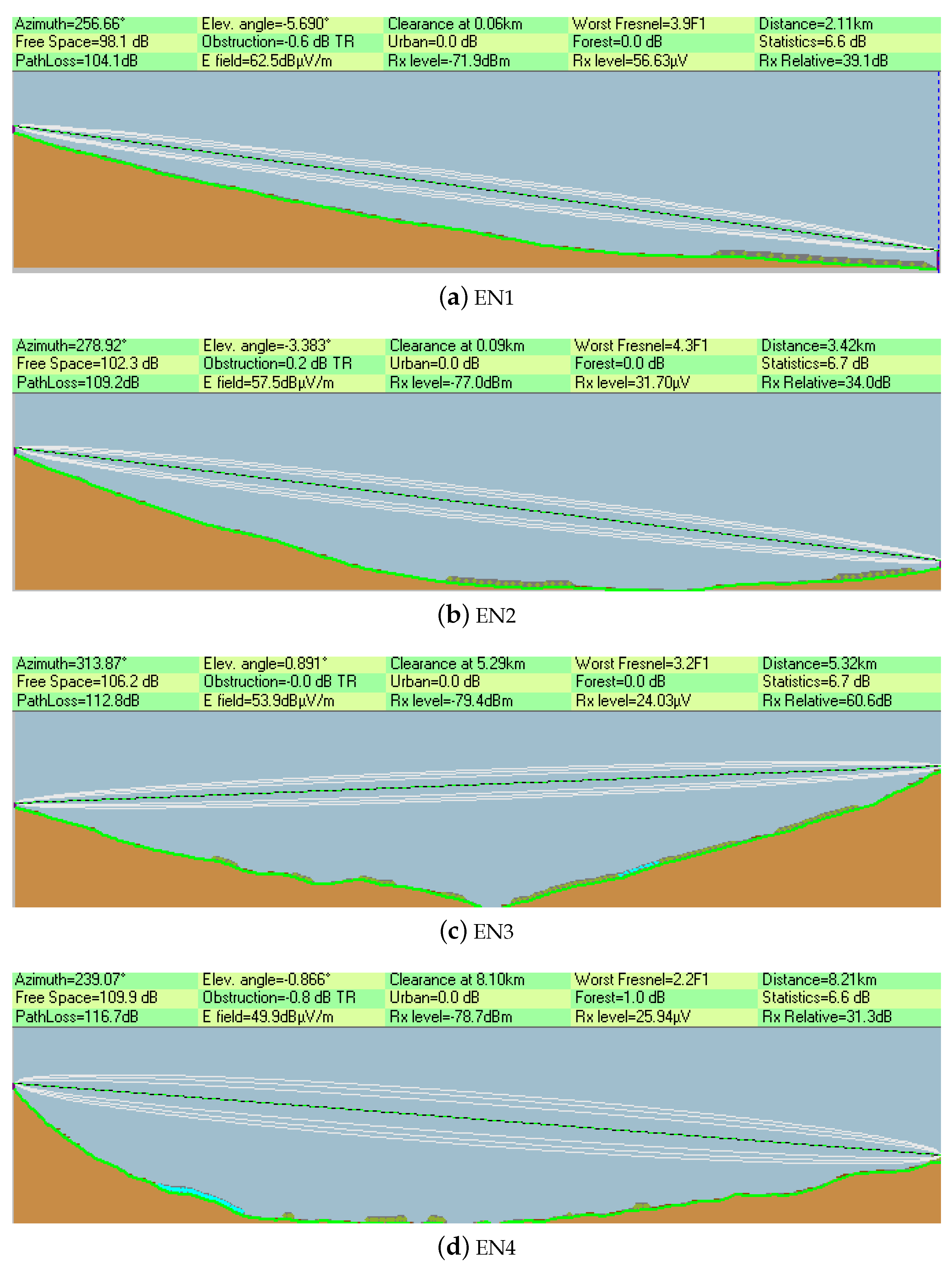
The ENs and the GW were deployed in the northern part of Medellín, where there is a valley with two mountains on each side, as shown in Figure 8. This topography allowed us to guarantee LoS conditions between each EN and the GW and avoid the obstruction in Fresnel zones, as shown in Figure 9 and as analyzed subsequently. The radius of the nth Fresnel zone can be calculated by

$$r_n=\sqrt{\frac{n·\lambda ·d}{4}},$$

(5)

where $r_n$ is the radius of the nth Fresnel zone, n is the considered Fresnel zone, $\lambda$ is the signal wavelength, and d is the distance between the transmitter and the receiver. To establish successful links, it is recommended that the first Fresnel zone (F1) is clear by more than 60% [12]. In our case, d is $2.11$ $\mathrm{k}$$\mathrm{m}$, $3.42$ $\mathrm{k}$$\mathrm{m}$, $5.32$ $\mathrm{k}$$\mathrm{m}$, and $8.21$ $\mathrm{k}$$\mathrm{m}$ for EN1, EN2, EN3, and EN4 correspondingly, and $\lambda$ = $0.33$ $\mathrm{m}$, so the F1 radii are $13.25$ $\mathrm{m}$, $16.87$ $\mathrm{m}$, $21.04$ $\mathrm{m}$, and $26.14$ $\mathrm{m}$. Because the worst F1 radii of our links are 3.9F1, 4.3F1, 3.2F1, and 2.2F1 (Figure 9), we are meeting and exceeding the minimum clearance of 60%, so our links can be modeled with LoS criteria. Thus, it can be concluded that the provided dataset is not dependent on the geometry of the terrain and can be used in other locations with similar weather characteristics.

The coordinates of each device in the network and its corresponding antenna height (h) and altitude (Alt) are shown in

Table 5. Locations, distances, and antenna heights of the end nodes.

Device	Lat	Long	h (m)	Alt (MASL)
GW	6.27°	−75.5479°	5	1699
EN1	6.2654°	−75.5664°	40	1476
EN2	6.2748°	−75.5785°	12.5	1494
EN3	6.3164°	−75.5764°	8	1723
EN4	6.2320°	−75.6117°	12	1566

.

5. Path Loss and Shadowing Modelling

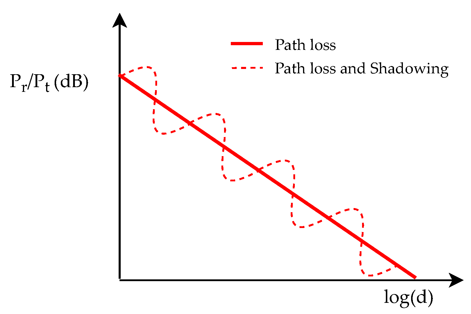
This section describes how this dataset can be used for path loss and shadowing modelling. Although path loss is caused by the attenuation of the power radiated by the transmitter and the channel effects, shadowing is caused by wave phenomena like absorption, reflection, scattering, and diffraction [12]. Both effects are shown in Figure 10. In that way, we fit an LDPLM and a multiple linear regression (MLR), including the environmental variables. Furthermore, we compare both approaches based on the RMSE and the correlation coefficient R². Of course, different models can be used for path loss modelling [12,13,14], so this procedure just serves as an example of how to use this dataset. Moreover, some machine learning techniques can also be used to estimate path loss and shadowing [40].

5.1. Data Preparation

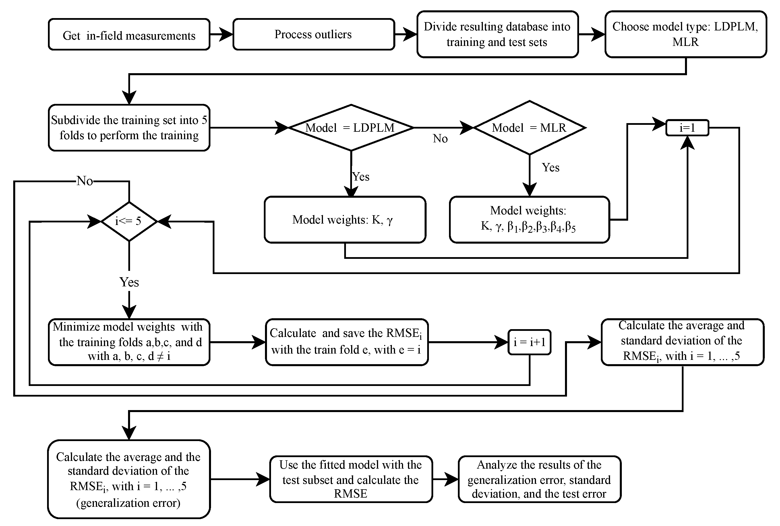
To develop the CPLS models that can be seen as application examples of our dataset, we followed the process depicted in Figure 11. After collecting the in-field measurements, we processed the outliers using the Mahalanobis distance $M_d$ [41]. This distance measures how far an observation and the dataset’s distribution is; in addition, it is not affected by the scales of the predictor variables and considers the covariance between them. According to [41], a row is considered an outlier if $M_d$ is greater than the tabulated value of the ${\chi }^2$ distribution with $n-1$ degrees of freedom and with a significance level $p=0.001$. Because the predictor variables that could be used from the dataset for modeling purposes are distance, frequency, SF, frame length, temperature, relative humidity, barometric pressure, particulate matter, time on air, energy, and experimental path loss, we have 11 degrees of freedom. Thus, the tabulated value of the ${\chi }^2$ distribution with 10 degrees of freedom and a p-value = 0.001 is 29.59. Then, we calculated $M_d$ for all the observations and removed those whose value was greater than 29.59.

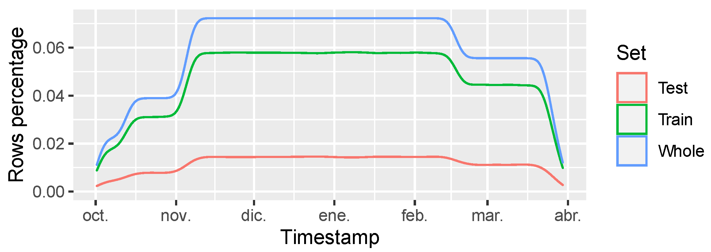
In the second step, we split the dataset into two subsets: one for training and one for testing. The idea behind this division is to adjust the models’ parameters with the training subset and assess the model’s ability to perform accurate predictions with new and unseen data (the test subset). In our case, we divided the whole dataset with 80% of rows for training, and 20% for testing, as commonly recommended in the literature [42] and previous path loss model approaches [25,26]. We divided the rows for both subsets by using a random split with a fixed seed to ensure the reproducibility of the results using the library $caTools$ of $RStudio$. We decided to use a uniformly distributed random split to correctly capture the CPLS changes caused by the environmental variables, which are very diverse in tropical regions like Colombia. Furthermore, using a uniformly distributed random split does not alter the distributions of predictor variables. The relation between the training subset, the testing subset, and the whole data frame in time is depicted in Figure 12, where it can be noticed that the subsets proportions are the same for each time interval.

In the third step, we divided our training subset into five folds to carry out k-fold-based cross-validation. This process helps reduce the risks of overfitting when calculating the models’ parameters [42]. Mainly, the operation principle is as follows: (i) divide the training subset into $a,b,c,d$ and e folds, (ii) calculate the models’ parameters with the folds $a,b,c,$ and d, and calculate the RMSE with the fold e, (iii) iterate the literal $ii$ alternating the folds, and (iv) calculate the average RMSE and the standard deviation of the RMSE for all the iterations. If the obtained model weights achieve low RMSE and standard deviation, it is considered that the model has a good ability for generalization. Finally, the fourth step uses the obtained model with unseen data, i.e., the testing set, and calculates the RMSE and R².

5.2. Log-Distance Combined Path Loss and Shadowing Model

A standard method to fit a combined path loss and shadowing (CPLS) model by using empirical data is the LDPLM (Equation (6)),

$$CPLS=K+10·\gamma ·lo{g}_{10}(\frac{d}{d_0})+\psi ,$$

(6)

where K is a dimensionless constant that depends on the characteristics of the antennas and the average channel attenuation, d is the distance, $d_0$ is the far-field distance, $\gamma$ is the path loss exponent, and $\psi$ is a random variable from a lognormal distribution, which characterizes shadowing, whose probability distribution function (PDF) is presented in Equation (7),

$$p\left(\psi \right)=\frac{\xi }{\sqrt{2\pi }·{\sigma }_{\psi }·\psi }·exp\left[-\frac{{(10·lo{g}_{10}\left(\psi \right)-{\mu }_{\psi })}^2}{2·{\sigma }_{\psi }^2}\right],\psi >0,$$

(7)

where $\xi =10/ln\left(10\right)$, ${\sigma }_{\psi }$ is the standard deviation of $\psi$, and ${\mu }_{\psi }$ is the mean of $\psi$. The CPLS has a LoS component attributed to the path loss and a stochastic component associated with the shadowing phenomenon, characterized by Equation (7). The LDPLM is assumed as a linear regression model where the input feature is the logarithm of the distance, K is the intercept, and $\psi$ is the residual error, i.e., the difference between the actual measurements and the model’s predictions. In that way, the LDPLM in Equation (6) can be fitted by using minimum squares optimization as expressed in Equation (8).

$$\begin{array}{c}\hfill \frac{\partial }{\partial \gamma }\sum _{j=1}^n{\left[M_i\left(d_i\right)-K-10·\gamma ·lo{g}_{10}\left(\frac{d_i}{d_0}\right)\right]}^2=0\\ \hfill \frac{\partial }{\partial K}\sum _{j=1}^n{\left[M_i\left(d_i\right)-K-10·\gamma ·lo{g}_{10}\left(\frac{d_i}{d_0}\right)\right]}^2=0,\end{array}$$

(8)

where $M_i\left(d_i\right)$ corresponds to the ith field measurement at the distance $d_i$. The far-field distance $d_0$ is calculated by

$$d_0=\frac{2D^2}{\lambda }$$

(9)

where D = 25 cm is the largest antenna size, and $\lambda =\frac{3\times {10}^8}{9\times {10}^8}$ = 0.33 m is the wavelength, so $d_0\ge$ $0.375$ $\mathrm{m}$. In that way, we considered a far-field distance $d_0$ = 1 $\mathrm{m}$.

After optimizing the model weights using our training subset, we found a path loss exponent $\gamma$ = 2.739 and K = 1.75. This value agrees with the typical interval for urban microcells [12]. Then, we used the training and test sets as follows: (i) we computed the LDPLM values, and (ii) we obtained the RMSE, standard deviation s, and the R² (

Table 6. Errors of fitted models.

Model	Subset	RMSE (dB)	R2
LDPLM	Training	2.465, s = 0.25	0.8517
	Test	2.46	0.8529
MLR	Training	1.843, s = 0.1	0.917
	Test	1.8401	0.9177

). The RMSE can be interpreted as the ability of the model to forecast the PL component, the standard deviation s captures the ability of the model to preserve the same error when using a different training subset, and the R² can be associated with shadowing. It can be noticed that the RMSE for both subsets is similar for LDPLM, so that the fitted model can forecast the PL with an RMSE = 2.46 dB. In the same way, the R² for both subsets was 0.85, so the model can explain the shadowing variability by 85%.

5.3. Multiple Linear Regression Model

Because previous works have shown that the environmental variables affect the CPLS, i.e., temperature [30], relative humidity [30], barometric pressure [43], particulate matter [33], and SNR [29], we proposed an enhancement of the LDPLM considering the log-distance term and the effects of the environmental variables as shown in Equation (10):

$$CPLS={\widehat{\beta }}_0+10\gamma lo{g}_{10}\left(d\right)+20lo{g}_{10}\left(f\right)+{\widehat{\beta }}_{1}T+{\widehat{\beta }}_{2}RH+{\widehat{\beta }}_{3}BP+{\widehat{\beta }}_{4}PM+{\widehat{\beta }}_{5}SNR+\psi ,$$

(10)

where ${\beta }_0$ is the model intercept (equivalent to K in Equation (6)), $\gamma$ is the path loss exponent, ${\beta }_i\in i=\left\{1,\dots ,5\right\}$ are the model predictors, f is the frequency (Hz), T is the temperature (°C), $RH$ is the relative humidity (%), $BP$ is the barometric pressure (hPa), $PM$ is the particulate matter ($\mathsf{\mu }$g/m³), $SNR$ is the signal-to-noise ratio (the received signal power divided by the noise floor power level in dB), and $\psi$ is the shadow fading term expressed in Equation (6). The path loss exponent is multiplied by ten from Equation (6), assuming a far-field distance $d_0$ = 1 m. The frequency weight is fixed to 20 from the Friis model [13]. To fit the MLR model, we have applied minimum squares optimization by differentiating the set of Equations in (11):

$$\frac{\partial }{\partial {\widehat{\theta }}_k}{\sum }_{i=0}^n{\left[C_i-\left(\widehat{K}+10\widehat{\gamma }{log}_{10}\left(d_i\right)+{\widehat{\beta }}_1{T}_i+{\widehat{\beta }}_{2}R{H}_i+{\widehat{\beta }}_{3}B{P}_i+{\widehat{\beta }}_{4}P{M}_i+{\widehat{\beta }}_{5}SN{R}_i\right)\right]}^2=0,$$

(11)

where K is the model intercept, ${\widehat{\theta }}_k\in \left\{{\widehat{\beta }}_1,\dots ,{\widehat{\beta }}_5,\widehat{\gamma }\right\}$ are the model predictors, $C_i=M_i-20{log}_{10}\left(f_i\right)$, $M_i$ is the ith experimental path loss observation, $d_i$, $f_i$, $T_i$, $R{H}_i$, $B{P}_i$, $P{M}_i$, and $SN{R}_i$ are the corresponding distance, frequency, temperature, relative humidity, barometric pressure, and SNR for the ith experimental path loss observation. The model coefficients found after the optimization are in

Table 7. Model predictors for the MLR CPLS model.

Predictor	Variable	Value
$\widehat{K}$	Intercept	−505.64
$\widehat{\gamma }$	Path loss exponent	2.203
${\widehat{\beta }}_1$	Temperature	0.123 dB/°C
${\widehat{\beta }}_2$	Relative humidity	0.0105 dB/%
${\widehat{\beta }}_3$	Barometric pressure	0.407 dB/hPa
${\widehat{\beta }}_4$	PM2.5	0.00222 dB/$\mathsf{\mu }$g/m3
${\widehat{\beta }}_5$	SNR	−0.635 dB/dB

.

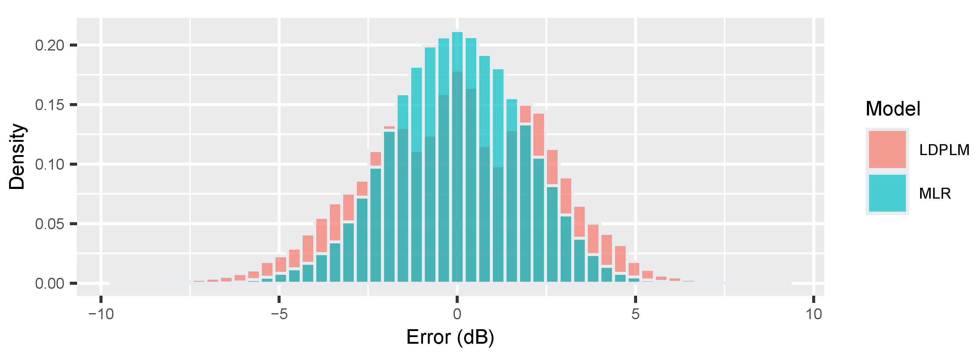
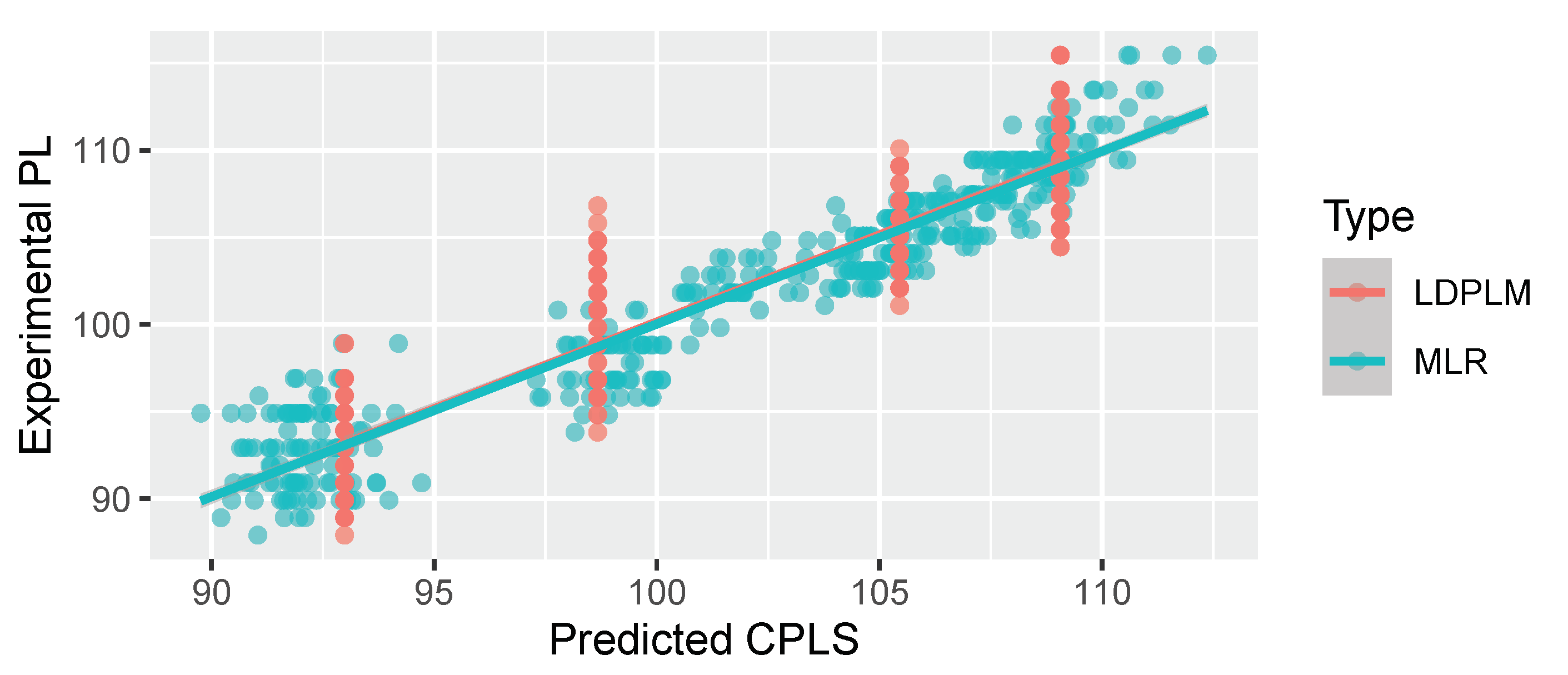
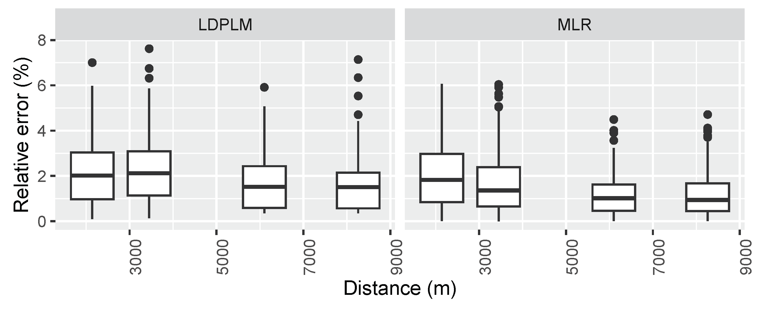
The model coefficients can be explained as discussed subsequently: (i) as expected, as the distance increases, the CPLS also increases, according to the predictions of different theoretical models like Friis [13] or two-ray [12]; furthermore, $\widehat{\gamma }$ = 2.203 attends the empirical values usually found for microcells [12], (ii) CPLS is directly proportional to the changes in temperature [30], (iii) relative humidity is also directly proportional to path loss [30], (iv) because a high barometric pressure causes high water vapor concentration, the effect of barometric pressure on CPLS is proportional, causing signal attenuation [32], and (v) the SNR has a negative impact on path loss, that is, when the SNR is worse, the path loss increases [29]. We obtained an RMSE for the test set of 1.84 dB and an R² equal to 0.9177, outperforming those obtained in the LDPLM. Remarkably, the R² increases from 0.85 (LDPLM) to 0.917 (MLR), exhibiting a better behavior regarding shadowing, so the inclusion of environmental variables helps improve the accuracy of the CPLS model. This fact can be verified in Figure 13, where we depict the histograms for the prediction errors of the LDPLM and the MLR CPLS models. It can be seen that (i) in the case of the LDPLM, the prediction error is not normally distributed, and (ii) in the case of the MLR model, it can be seen that the prediction error is normally distributed, fixing the problem of normality, and the errors are more concentrated around the mean. Furthermore, in Figure 14, it can be seen that the predicted values using the MLR CPLS model are more concentrated around the regression line because this method exhibits a higher R². Finally, we depicted the error distributions of each model regarding the distance in the box plots of Figure 15, where it can be noticed that distance does not affect the relative errors of the models, which are around 1.5%. Increasing the accuracy of the CPLS models by using the environmental variables can be used for energy reduction by applying TPC strategies and for localization or tracking tasks [29].

6. Conclusions

This paper described an empirical dataset of different variables in a LoRaWAN deployment, including the collection methodology and possible applications. Our dataset contains the information of four ENs and one GW in Medellín, Colombia, in an urban environment, for four months. In addition to the traditional variables considered in other measurement campaigns, our experimental setup included sensors for measuring temperature, relative humidity, barometric pressure, and particulate matter PM2.5. These variables can be used for fitting accurate path loss and shadowing models that can be applied to different tasks like TPC or positioning. We also showed how our dataset could be used for CPLS modelling, including LDPLM and MLR models, indicating that the inclusion of the environmental variables helps improve the forecast of shadowing versus the traditional LDPLM from an R² of 0.85 to 0.91. Furthermore, our dataset also includes the energy consumption in each transmission, the SF, the SNR, and the frame size, so it can be used to study energy behavior in different transmitter configurations.

References

- Casaccia, S.; Romeo, L.; Calvaresi, A.; Morresi, N.; Monteriu, A.; Frontoni, E.; Scalise, L.; Revel, G.M. Measurement of users’ well-being through domotic sensors and machine learning algorithms. IEEE Sens. J. 2020, 20, 8029–8038. [Google Scholar] [CrossRef]
- Rajesh, P.; Shajin, F.H.; Kannayeram, G. A novel intelligent technique for energy management in smart home using internet of things. Appl. Soft Comput. 2022, 128, 109442. [Google Scholar] [CrossRef]
- Caruso, A.; Chessa, S.; Escolar, S.; Barba, J.; López, J.C. Collection of data with drones in precision agriculture: Analytical model and LoRa case study. IEEE Internet Things J. 2021, 8, 16692–16704. [Google Scholar] [CrossRef]
- Mahdavinejad, M.S.; Rezvan, M.; Barekatain, M.; Adibi, P.; Barnaghi, P.; Sheth, A.P. Machine learning for Internet of Things data analysis: A survey. Digit. Commun. Netw. 2018, 4, 161–175. [Google Scholar] [CrossRef]
- Athanasaki, D.E.; Mastorakis, G.; Mavromoustakis, C.X.; Markakis, E.K.; Pallis, E.; Panagiotakis, S. IoT Detection Techniques for Modeling Post-Fire Landscape Alteration Using Multitemporal Spectral Indices. In Convergence of Artificial Intelligence and the Internet of Things; Springer: Berlin/Heidelberg, Germany, 2020; pp. 347–367. [Google Scholar] [CrossRef]
- Hadipour, M.; Derakhshandeh, J.F.; Shiran, M.A. An experimental setup of multi-intelligent control system (MICS) of water management using the Internet of Things (IoT). ISA Trans. 2020, 96, 309–326. [Google Scholar] [CrossRef] [PubMed]
- Adeel, A.; Gogate, M.; Farooq, S.; Ieracitano, C.; Dashtipour, K.; Larijani, H.; Hussain, A. A survey on the role of wireless sensor networks and IoT in disaster management. In Geological Disaster Monitoring Based on Sensor Networks; Springer: Berlin/Heidelberg, Germany, 2019; pp. 57–66. [Google Scholar] [CrossRef] [Green Version]
- Ikpehai, A.; Adebisi, B.; Rabie, K.M.; Anoh, K.; Ande, R.E.; Hammoudeh, M.; Gacanin, H.; Mbanaso, U.M. Low-power wide area network technologies for Internet-of-Things: A comparative review. IEEE Internet Things J. 2018, 6, 2225–2240. [Google Scholar] [CrossRef] [Green Version]
- Sornin, N.; Luis, M.; Eirich, T.; Kramp, T.; Hersent, O. Lorawan Specification; LoRa Alliance: Fremont, CA, USA, 2015; pp. 6–77. [Google Scholar]
- Mekki, K.; Bajic, E.; Chaxel, F.; Meyer, F. A comparative study of LPWAN technologies for large-scale IoT deployment. ICT Express 2019, 5, 1–7. [Google Scholar] [CrossRef]
- Wixted, A.J.; Kinnaird, P.; Larijani, H.; Tait, A.; Ahmadinia, A.; Strachan, N. Evaluation of LoRa and LoRaWAN for wireless sensor networks. In Proceedings of the 2016 IEEE SENSORS, Orlando, FL, USA, 30 October–3 November 2016; pp. 1–3. [Google Scholar] [CrossRef]
- Goldsmith, A. Wireless Communications; Cambridge University Press: Cambridge, UK, 2005. [Google Scholar] [CrossRef] [Green Version]
- Friis, H.T. A note on a simple transmission formula. Proc. Ire 1946, 34, 254–256. [Google Scholar] [CrossRef]
- Okumura, Y. Field strength and its variability in VHF and UHF land-mobile radio service. Rev. Electr. Commun. Lab. 1968, 16, 825–873. [Google Scholar]
- Rappaport, T.S. Wireless Communications: Principles and Practice; Prentice Hall PTR: Englewood Cliffs, NJ, USA, 1996; Volume 2. [Google Scholar]
- Jawad, H.M.; Jawad, A.M.; Nordin, R.; Gharghan, S.K.; Abdullah, N.F.; Ismail, M.; Abu-AlShaeer, M.J. Accurate empirical path-loss model based on particle swarm optimization for wireless sensor networks in smart agriculture. IEEE Sens. J. 2019, 20, 552–561. [Google Scholar] [CrossRef]
- Faraway, J.J. Practical Regression and ANOVA Using R; University of Bath: Bath, UK, 2002; Volume 168. [Google Scholar]
- Xu, W.; Kim, J.Y.; Huang, W.; Kanhere, S.S.; Jha, S.K.; Hu, W. Measurement, characterization, and modeling of lora technology in multifloor buildings. IEEE Internet Things J. 2019, 7, 298–310. [Google Scholar] [CrossRef] [Green Version]
- Kim, D.H.; Lee, E.K.; Kim, J. Experiencing LoRa network establishment on a smart energy campus testbed. Sustainability 2019, 11, 1917. [Google Scholar] [CrossRef] [Green Version]
- El Chall, R.; Lahoud, S.; El Helou, M. LoRaWAN network: Radio propagation models and performance evaluation in various environments in Lebanon. IEEE Internet Things J. 2019, 6, 2366–2378. [Google Scholar] [CrossRef]
- Masek, P.; Stusek, M.; Svertoka, E.; Pospisil, J.; Burget, R.; Lohan, E.S.; Marghescu, I.; Hosek, J.; Ometov, A. Measurements of LoRaWAN Technology in Urban Scenarios: A Data Descriptor. Data 2021, 6, 62. [Google Scholar] [CrossRef]
- Bhatia, L.; Breza, M.; Marfievici, R.; McCann, J.A. Dataset: Loed: The lorawan at the edge dataset. arXiv 2020, arXiv:2010.14211. [Google Scholar] [CrossRef]
- Aernouts, M.; Berkvens, R.; Van Vlaenderen, K.; Weyn, M. Sigfox and LoRaWAN datasets for fingerprint localization in large urban and rural areas. Data 2018, 3, 13. [Google Scholar] [CrossRef] [Green Version]
- Li, Y.; Barthelemy, J.; Sun, S.; Perez, P.; Moran, B. Urban vehicle localization in public LoRaWan network. IEEE Internet Things J. 2021, 9, 10284–10293. [Google Scholar] [CrossRef]
- Anzum, R.; Habaebi, M.H.; Islam, M.R.; Hakim, G.P.; Khandaker, M.U.; Osman, H.; Alamri, S.; AbdElrahim, E. A Multiwall Path-Loss Prediction Model Using 433 MHz LoRa-WAN Frequency to Characterize Foliage’s Influence in a Malaysian Palm Oil Plantation Environment. Sensors 2022, 22, 5397. [Google Scholar] [CrossRef]
- Alobaidy, H.A.; Nordin, R.; Singh, M.J.; Abdullah, N.F.; Haniz, A.; Ishizu, K.; Matsumura, T.; Kojima, F.; Ramli, N. Low-Altitude-Platform-Based Airborne IoT Network (LAP-AIN) for Water Quality Monitoring in Harsh Tropical Environment. IEEE Internet Things J. 2022, 9, 20034–20054. [Google Scholar] [CrossRef]
- Batalha, I.S.; Lopes, A.V.; Lima, W.G.; Barbosa, Y.H.; Neto, M.C.; Barros, F.J.; Cavalcante, G.P. Large-Scale Modeling and Analysis of Uplink and Downlink Channels for LoRa Technology in Suburban Environments. IEEE Internet Things J. 2022, 9, 24477–24490. [Google Scholar] [CrossRef]
- Callebaut, G.; Van der Perre, L. Characterization of LoRa point-to-point path loss: Measurement campaigns and modeling considering censored data. IEEE Internet Things J. 2019, 7, 1910–1918. [Google Scholar] [CrossRef]
- Bianco, G.M.; Giuliano, R.; Marrocco, G.; Mazzenga, F.; Mejia-Aguilar, A. LoRa system for search and rescue: Path-loss models and procedures in mountain scenarios. IEEE Internet Things J. 2020, 8, 1985–1999. [Google Scholar] [CrossRef]
- Deese, A.S.; Jesson, J.; Brennan, T.; Hollain, S.; Stefanacci, P.; Driscoll, E.; Dick, C.; Garcia, K.; Mosher, R.; Rentsch, B.; et al. Long-term monitoring of smart city assets via Internet of Things and low-power wide-area networks. IEEE Internet Things J. 2020, 8, 222–231. [Google Scholar] [CrossRef]
- Fang, Z.; Guerboukha, H.; Shrestha, R.; Hornbuckle, M.; Amarasinghe, Y.; Mittleman, D.M. Secure Communication Channels Using Atmosphere-limited Line-of-sight Terahertz Links. IEEE Trans. Terahertz Sci. Technol. 2022, 12, 363–369. [Google Scholar] [CrossRef]
- Union, I.T. Attenuation by atmospheric gases and related effects, ITUR P.676-13. In Recommendation ITU-R; International Telecommunication Union: Geneva, Switzerland, 2022; pp. 676–688. [Google Scholar]
- Min, N.; Ren, J.; Yang, G.; Zhang, M.-L.; Pei, C.-X. Influences of PM2. 5 atmospheric pollution on the performance of free space quantum communication. Acta Phys. Sin. 2015, 64, 150301. [Google Scholar] [CrossRef]
- LoRa-Alliance. RP002-1.0.1 LoRaWAN® Regional Parameters; LoRa Alliance, Inc.: Fremont, CA, USA, 2020. [Google Scholar]
- Reynders, B.; Pollin, S. Chirp spread spectrum as a modulation technique for long range communication. In Proceedings of the 2016 Symposium on Communications and Vehicular Technologies (SCVT), Mons, Belgium, 22–23 November 2016; pp. 1–5. [Google Scholar] [CrossRef]
- Heusse, M.; Attia, T.; Caillouet, C.; Rousseau, F.; Duda, A. Capacity of a lorawan cell. In Proceedings of the 23rd International ACM Conference on Modeling, Analysis and Simulation of Wireless and Mobile Systems, Alicante, Spain, 16–20 November 2020; pp. 131–140. [Google Scholar] [CrossRef]
- The-Things-Network. Adaptative Data Rate. Available online: https://www.thethingsnetwork.org/docs/lorawan/adaptive-data-rate/ (accessed on 15 December 2022).
- Firouzi, F.; Chakrabarty, K.; Nassif, S. Intelligent Internet of Things: From Device to Fog and Cloud; Springer: Berlin/Heidelberg, Germany, 2020. [Google Scholar] [CrossRef]
- Abdelghany, A.; Uguen, B.; Moy, C.; Lemur, D. On Superior Reliability of Effective Signal Power versus RSSI in LoRaWAN. In Proceedings of the 2021 28th International Conference on Telecommunications (ICT), London, UK, 1–3 June 2021; pp. 1–5. [Google Scholar] [CrossRef]
- Yang, G.; Zhang, Y.; He, Z.; Wen, J.; Ji, Z.; Li, Y. Machine-learning-based prediction methods for path loss and delay spread in air-to-ground millimetre-wave channels. IET Microwaves Antennas Propag. 2019, 13, 1113–1121. [Google Scholar] [CrossRef]
- De Maesschalck, R.; Jouan-Rimbaud, D.; Massart, D.L. The mahalanobis distance. Chemom. Intell. Lab. Syst. 2000, 50, 1–18. [Google Scholar] [CrossRef]
- Thanaki, J. Machine Learning Solutions: Expert Techniques to Tackle Complex Machine Learning Problems Using Python; Packt Publishing Ltd.: Birmingham, UK, 2018. [Google Scholar]
- Ohshima, K.; Hara, H.; Hagiwara, Y.; Terada, M. Field experiments for developing transmission control based on weather estimation in an environmental wireless sensor network. In Proceedings of the 2010 Australasian Telecommunication Networks and Applications Conference, Auckland, New Zealand, 31 October–3 November 2010; pp. 19–24. [Google Scholar] [CrossRef]
Figure 1.
LoRaWAN architecture. A typical LoRaWAN deployment includes end nodes, gateways, a network server, and application servers.
Figure 2.
Empirical distributions of the collected variables per node. In (a), we depict the SF usage from 7 to 10. In (b), we show the number of collected samples at each distance. In (c), we show the number of collected samples at each frequency. In (d–j), we depict the experimental distributions per node for temperature, relative humidity, barometric pressure, particulate matter, path loss, energy, and SNR, correspondingly.
Figure 3.
ESP and noise power of ENs.
Figure 4.
LoRaWAN deployment to capture the information contained in the dataset.
Figure 5.
Mounting angles of the ENs’ antennas. The omnidirectional antennas were mounted perpendicular to the ground. The Yagi–Uda antenna was mounted with the boom parallel to the ground.
Figure 6.
S11 characterization for an EN. It can be noticed that the antennas used have acceptable behavior regarding the S11 parameter, with returns of less than 3%.
Figure 7.
End Node testbed. The elements are (1) microcontroller, (2) pressure sensor, (3) energy sensor, (4) relative humidity and temperature sensor, (5) PM2.5 sensor inlet, and (6) antenna connection outlet.
Figure 8.
Network deployment. We deployed one GW and four ENs. Credits: Google Earth.
Figure 9.
Line of sight for the communication between the GW and the ENs. Credits: Radio Mobile.
Figure 10.
Theoretical behavior of path loss and shadowing. The dissipation caused by the channel, i.e., the ratio between the transmitted power P and the received power Pr, changes according to the logarithm of the distance d [12].
Figure 11.
Model fitting process. We (i) collected and cleaned the database, (ii) divided the dataset into training and testing, (iii) trained the models, and (iv) evaluated the models’ performances.
Figure 12.
Percentage of rows for training and testing subsets compared with the whole dataframe. The measurement campaigns started in October 2021 and finished on March 2022.
Figure 13.
Shadowing distribution using the LDPLM and MLR models. It can be noticed that the errors are more concentrated around the mean when using the MLR model, and the distribution is bell-shaped.
Figure 14.
Predicted versus measured CPLS for LDPLM and MLR models. It can be noticed that the MLR CPLS predictions are more concentrated around the regression line than those predicted by the LDPLM CPLS model.
Figure 15.
Box plots of relative errors of the LDPLM and MLR CPLS models versus distance. It can be noticed that the mean errors are around 1.5%.