
Convolutional-Based Encoder–Decoder Network for Time Series Anomaly Detection during the Milling of 16MnCr5
WBK Institute for Production Science, Karlsruhe Institute of Technology (KIT), Kaiserstraße 12, 76131 Karlsruhe, Germany
*
Author to whom correspondence should be addressed.
Data 2022, 7(12), 175; https://doi.org/10.3390/data7120175
Submission received: 25 October 2022
/
Revised: 23 November 2022
/
Accepted: 23 November 2022
/
Published: 6 December 2022
(This article belongs to the Special Issue Artificial Intelligence and Big Data Applications in Diagnostics)
Abstract
:Machine learning methods have widely been applied to detect anomalies in machine and cutting tool behavior during lathe or milling. However, detecting anomalies in the workpiece itself have not received the same attention by researchers. In this article, the authors present a publicly available multivariate time series dataset which was recorded during the milling of 16MnCr5. Due to artificially introduced, realistic anomalies in the workpiece, the dataset can be applied for anomaly detection. By using a convolutional autoencoder as a first model, good results in detecting the location of the anomalies in the workpiece were achieved. Furthermore, milling tools with two different diameters where used which led to a dataset eligible for transfer learning. The objective of this article is to provide researchers with a real-world time series dataset of the milling process which is suitable for modern machine learning research topics such as anomaly detection and transfer learning.
Dataset: 10.5445/IR/1000151546.
Dataset License: CC BY 4.0: Creative Commons 4.0 International
1. Summary
The process of anomaly detection is an important topic in machine learning research and has significant potential to further decrease manufacturing costs on the way towards zero-defect manufacturing [1]. With regards to milling, considerable research has been carried out to detect anomalous cutting tool behavior. Among other methods, acoustic signals were classified as normal or anomalous with generative adversarial networks [2], a CNN-AD was trained on spindle current [3] and a decision tree for feature selection in combination with a Naïve Bayes classifier was introduced to detect faulty tool conditions [4]. However, detecting anomalies in the workpiece itself is rarely considered. To the best of our knowledge, no dataset has been published to detect anomalies in the workpiece during milling by only using time series gathered by machine internal sensors, which is the contribution of this article.
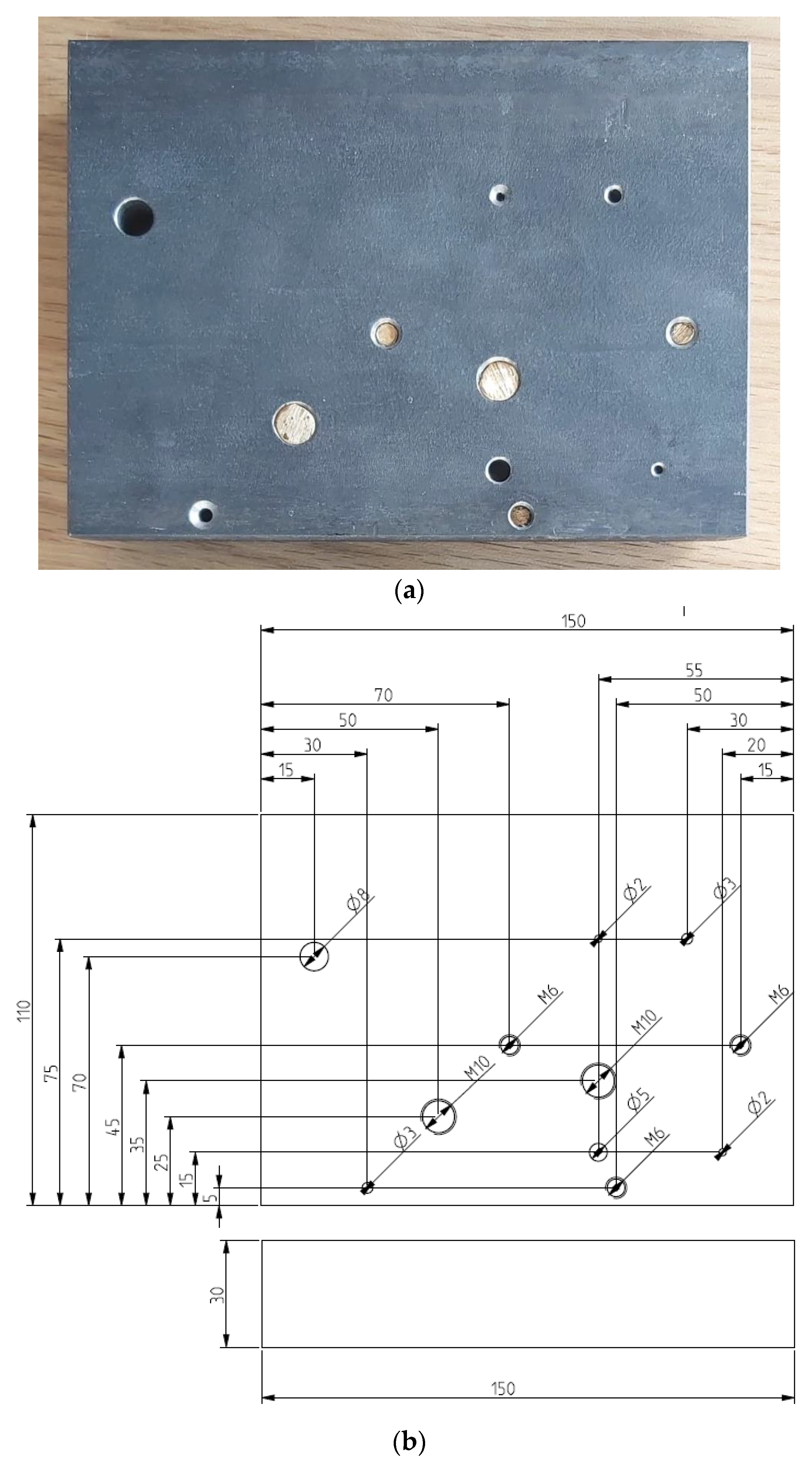
The presented dataset was obtained by milling a workpiece made of 16MnCr5 which is a commonly used steel in machining. Eleven anomalies consisting of six boreholes [5] and five threaded holes in which a threaded rod made of brass was mounted were artificially introduced into the workpiece. The workpiece and its corresponding technical drawing are shown in Figure 1. The dimensions of the workpiece are 150 × 110 × 30 mm. Borehole diameters differ in size and consist of two boreholes with diameter 2 mm and 3 mm respectively as well as one borehole with diameter 5 mm and 8 mm, respectively, to study the performance of anomaly detection under varying conditions. For the same reason, three threaded rods with a diameter of 6 mm and two threaded rods with a diameter of 10 mm were used.
The data were captured by using the Simatic edge device (IPC227E). This device is able to collect different data streams such as the position of the axis, the motor current as well as the torque. In the here presented figures only the motor current is depicted which is the most informative signal and has been used to investigate the anomaly detection model. All milling runs were performed on a CMX 600 V milling center developed by DMG Mori. Process parameters as well as used milling tools are presented in Chapter 2.
The dataset was recorded and published to provide researchers with a real-world dataset containing multiple features of a milling machine during machining. In addition to machining under normal conditions, the authors recorded the effects of differently sized anomalies introduced into the workpiece as well as four milling tool breakages. This time series dataset therefore is relevant for multiple applications in industry as well as research and suitable for anomaly detection and detection of milling tool breakage. Specifically, the authors show how the dataset can be used for anomaly detection in the material. An obvious application of the dataset is using it for transfer of learning for other materials, and then 16MnCr5. This is due to the fact that while using another material, the resulting signals should be similar though not identical. Another application of the dataset is using it for tool anomaly detection, though this is not further considered in this work.
In the this presented work, the authors concentrate on detecting anomalies in the material. By training a convolutional-based encoder–decoder model the authors achieved success in detecting 98% of artificially created anomalies in the time series before a tool breakage occurred. The model was further able to localize the anomalies in the workpiece based on the recorded position of the milling tool over time. In this approach, the accuracy of the location of detected anomalies is dependent on the tool diameter which is explained further in the paper. Furthermore, it was found that using a model trained on data collected during machining with a tool 10 mm in diameter for anomaly detection on data collected during machining with a tool 8 mm in diameter results in worse model performance. Performance also dropped when the authors switched from high-speed steel (HSS) milling cutters to solid carbide (SC) milling cutters, thus, indicating a domain shift and opening up additional applications for domain adaption.
2. Data Description
The dataset, available under (10.5445/IR/1000151546) (the authors strongly recommend to consider the published data along with the presented description here) consists of seven folders. Each folder represents one milling run over the whole workpiece. In each milling run, the depth of cut was set to 3 mm. A folder contains a maximum of three json files. The number of files depends on the time needed for each run which is a function of milling tool diameter and feed rate. Files in each folder were numerated in sequence. For example, folder “run1” contains the files “run1_1” and “run1_2” with the last number indicating the order in which the files were generated. The frequency of recording datapoints was set to 500 Hz.
During each milling run, the milling tool moved along the longitudinal side and then was moved back alongside the workpiece. This way, machining always started on the same side of the workpiece. Spindle speed and feed rate which are dependent on material (16MnCr5), depth of cut (3 mm) and full-slot milling were set according to the online calculation tool provided by the milling tool manufacturer [6].
Table 1 provides an overview of the milling runs. Run 1 to 4 were performed with an HSS tool with a diameter of 10 mm. The tool in use was an end mill (HSS-E-SPM HPC 10 mm) developed by Hoffmann Group. During the first three runs with this end mill, no tool breakage occurred. However, in run 4, the tool broke. Runs 5 and 6 were performed by milling with an end mill of the same tool series (HSS-E-SPM HPC 8 mm) that just differs in tool diameter. In contrast to this, run 7 was performed by using a solid carbide tool (solid carbide roughing end mill HPC 8 mm). Cutting with SC tools provides much higher productivity with the downside being a higher tool price. In the this presented case, the SC end mill performed cuts with a feed rate of 1150 mm/min compared to 191 mm/min achieved by a HSS end mill of the same diameter. Tool breakages were recorded on all runs with end mills 8 mm in diameter.
Each json file consists of a header and a payload. The header lists all parameters that were recorded such as position, motor torque and motor current of each of a maximum of five axes of a milling machine. However, the machine used in the experiments is a 3-axis machining center which leaves the payload of two possible additional axes to be empty. In the payload, the sequential data for each parameter can be found. A list of recorded signals can be found in Table 2.
To summarize the dataset, in all experiments 16MnCr5 was used as the material. Four runs were performed with a tool diameter of 10 mm without facing tool defects. Three runs were performed with tool diameters of 8 mm where in each run a tool breakdown occurred. Hence the data of the last three runs can be used for both anomaly detection in the material as well as in the tool. For all runs, different data streams as depicted in Table 2 were collected even though only the motor current was used for anomaly detection.
3. Methods and Results
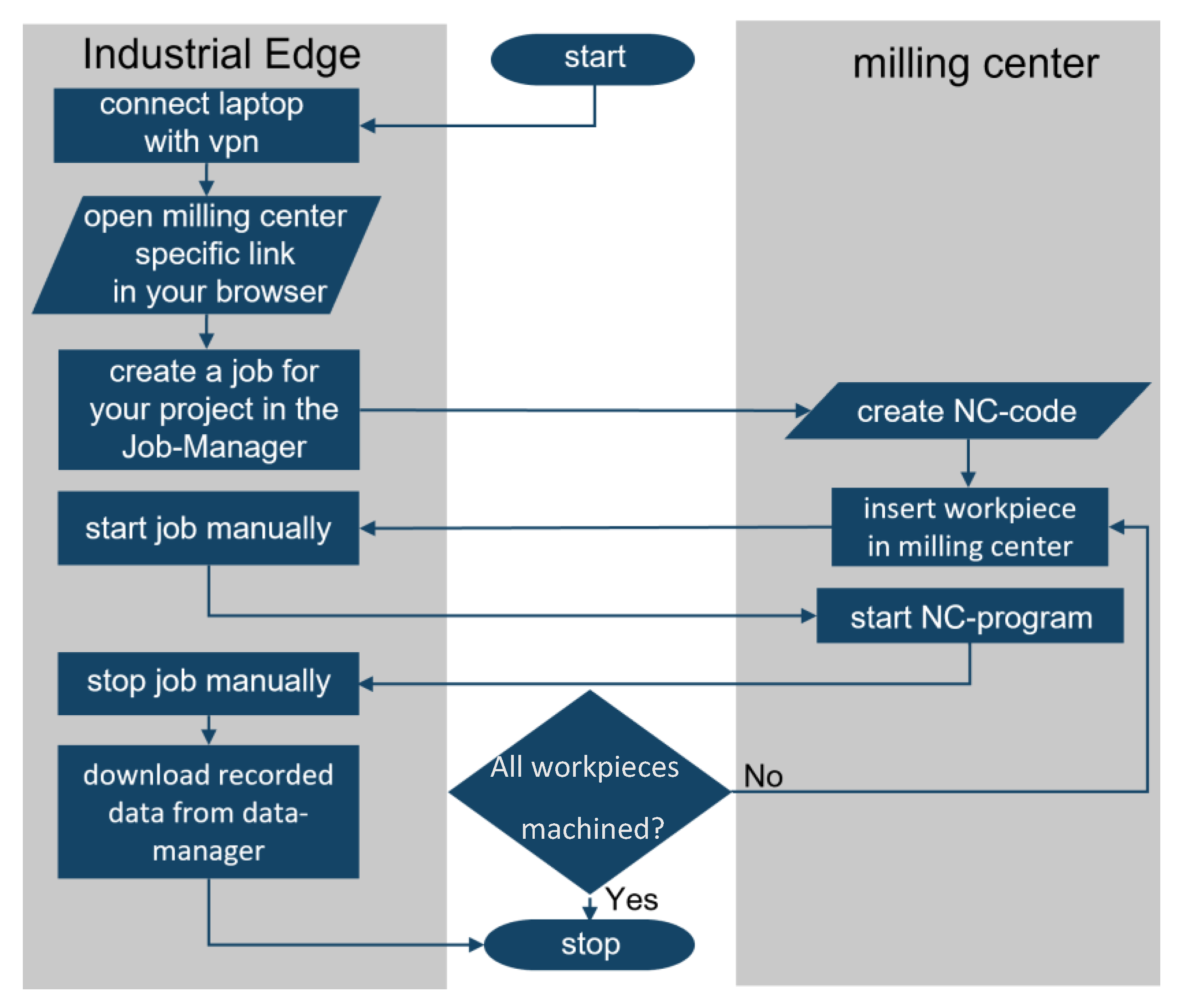
The dataset was collected by using an Simatic edge device which was connected to the milling center. The sampling rate was set to 500 Hz for every collected signal listed in Table 2. This way the authors ended up with a dataset containing not only motor current but also the position as well as the torque of each axis and several additional signals mentioned above. Since the recording was started shortly before the NC program, there is a short duration until the signals change their values. This must be considered in the following work. The workflow for data recording is depicted in Figure 2.
After collecting the data, a convolutional-based encoder–decoder network to determine where anomalies exist in the workpiece was trained. The ability to detect anomalies in time series by applying convolutions was successfully demonstrated by multiple publications [1,7,8,9].
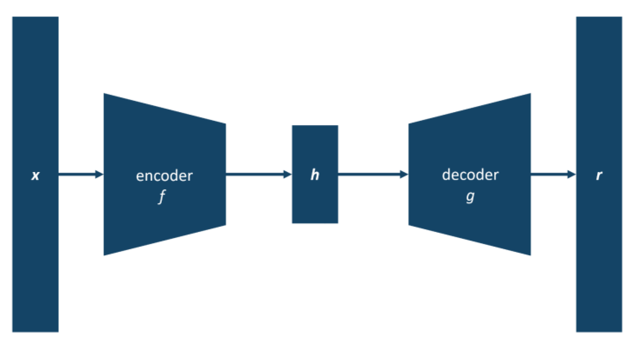
An undercomplete autoencoder is a feedforward deep neural network that tries to reconstruct its input and consists of two parts being an encoder and a decoder [10]. The encoder is used for data compression with the function and the second part is the decoder for reconstruction with the function with the most compressed representation being called bottleneck, hidden layer or latent representation , where p > q [11]. This notation leads to the reconstructed input signal with . The basic architecture of an autoencoder is depicted in Figure 3. A commonly used loss function is mean squared error (MSE) [11].
As a first model, an encoder consisting of two Conv1D layers and a decoder consisting of two Conv1DTranspose layers with an Adam optimizer, learning rate 0.001 and ReLu as activation function was used [12]. The number of filters was set to 16-32-16-1 and a stride of two as well as padding was applied to all layers. Training data were split in sequences of lengths of 256 data points. In addition, early stopping with a patience of 5 was implemented. The model was trained for 10 epochs on data of run 2 and a loss of 0.0184 with mean squared error as the loss function was achieved [11].
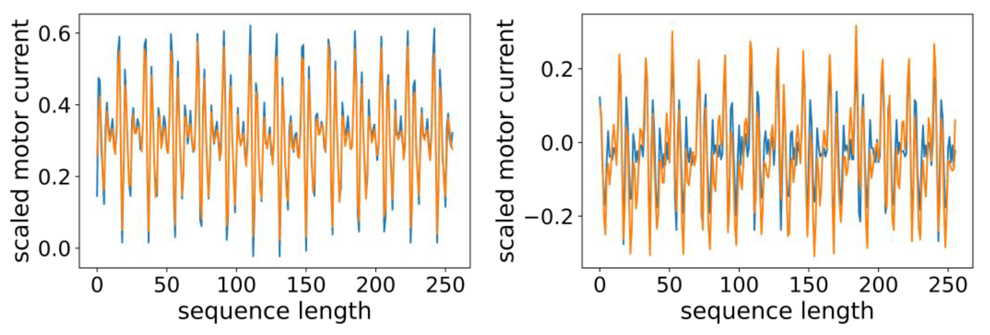
Figure 4 shows an example of a sequence which was reconstructed well (left) and a sequence which was not reconstructed well (right) by the model. The left sequence is from a part of the workpiece without an anomaly and the right sequence represents the motor current of the y-axis while cutting through the first borehole, which can be seen at the top center in Figure 5.
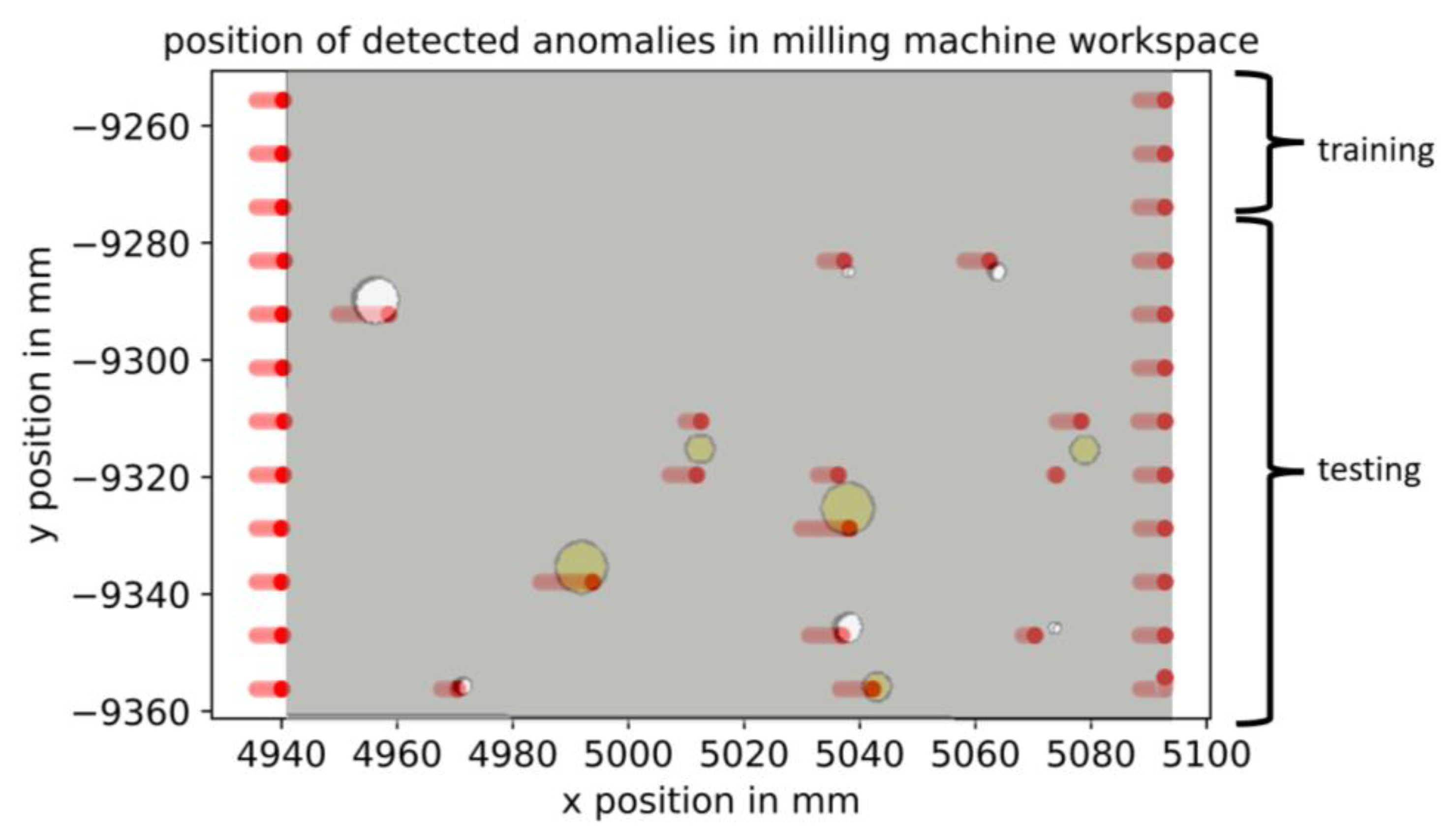
According to Figure 5, either three tool paths without anomalies were milled with a tool diameter of 10 mm or four tool paths with a tool diameter of 8 mm. These anomaly free tool paths were then used to train the model and the remaining part of the workpiece was used for validation. All found anomalies are highlighted in red in Figure 5. After training the network, the detected anomalies in the milling machine workspace were localized. This was carried out by saving the time of each detected anomaly in the time series and determining the value of the positional signals in x and y coordinates. After that, the authors put the plot of all anomalies on top of the CAD model of the workpiece to validate the model performance. Figure 5 gives an overview of the workpiece with its anomalies and shows the anomaly-free part used for training. It is also obvious that all anomalies have been detected correctly based on the defect-free training data.
The maximum achieved anomaly localization resolution is bound to the tool diameter which leads to a drift in localization for certain anomalies. This can be proven by the fact that anomalies are detected with a slight shift to the left which can be traced back to the milling tool being moved from left to right. This way the center of the milling cutter is on the left when the cutter has its first contact with the anomaly. It can also be seen that some anomalies are detected twice. This is due to the fact that the anomaly is part of two milling paths. Besides the actual anomalies, several additional anomalies were found resulting from the tool entering or leaving the workpiece. These additional anomalies are located on the right and left side of each tool path. However, these anomalies can be deleted by implementing an interface between the autoencoder and the CAD model which was not part of this study.
After achieving the above-mentioned results, the authors decided to use a model trained on data generated with a tool diameter of 10 mm to detect anomalies in a workpiece which is machined with a tool diameter of 8 mm. With this approach, the ability of generalization over different tool diameters should be investigated. If it can be shown that the model is not able to generalize directly, this shows that a domain shift which results from the tool diameter change and the dataset can be used to further investigate issues with respect to domain shift. It was found that the model was not able to achieve sufficient results regarding the reconstruction error. This indicates a domain shift in the data. Model performance also worsened when the model trained on HSS milling tools was used on data generated by milling with an SC cutter, which implies a second domain shift.
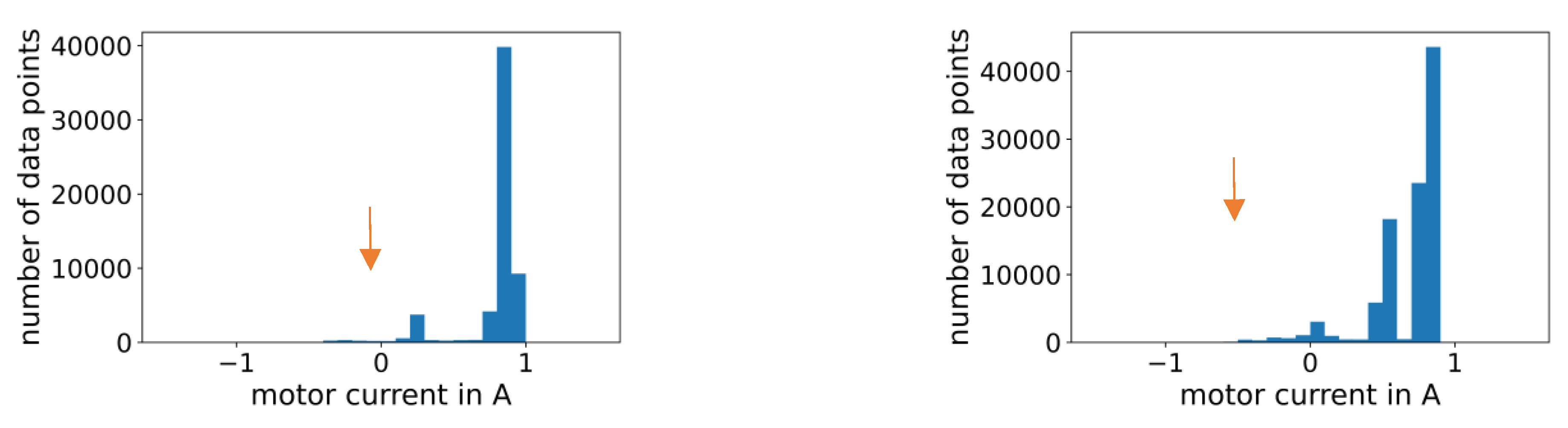
Furthermore, a change in current distribution can be noticed by comparing histograms of 10 mm and 8 mm training data. Milling with a 10 mm end mill requires more current due to a bigger radial depth of cut which then leads to an increase in samples with higher current as pointed out in Figure 6 (left) by the orange arrow. Note that Figure 6 compares the histograms of the part of the workpiece which is without anomalies. Due to an increase from three needed milling paths for a tool with diameter 10 mm to four milling paths with a tool diameter of 8 mm, the sum of collected datapoints for the same machined area is varying.
Besides this domain shift between 8 mm and 10 mm data, an additional effect was detected in training data of all milling runs with tool diameter of 8 mm. The reason lies in the combination of workpiece dimensions and tool diameter. To separate the workpiece in the same machined areas for training and testing regardless of the tool diameter, the first tool path of 8 mm tools was conducted with a radial depth of cut of 6 mm compared to three following tool paths with 8 mm radial depth of cut. The decrease in radial depth of cut led to a temporal shift in current consumption on tool path one compared to tool paths two to four. Such a temporal shift in time series distribution was recently labeled temporal covariate shift (TCP) and is pointed out by the orange arrow in Figure 6 (right) [13]. Training a model which can handle data shifts is key to implementing this anomaly detection approach in industry because varying radial and axial depths of cut throughout milling a workpiece are common. Further publications regarding handling this domain shift are to be expected in the future.
4. Conclusions
In conclusion, the presented multivariate real-world dataset of milling 16MnCr5 is suitable for training and testing machine learning models for detecting material anomalies in time series data. This has been successfully demonstrated by training a convolutional autoencoder as a first model which can detect 98% of the anomalies excluding those anomalies that were not machined due to a prior tool breakage. Due to artificially introduced anomalies which vary in size and type, the presented dataset offers a unique challenge for machine learning algorithms to detect these anomalies. Furthermore, by using multiple milling tools which differ in diameter and material, the presented dataset can also be applied for transfer learning and further investigation of domain shift issues. In addition, during milling with tools 8 mm in diameter, a temporal covariate shift (TCP) can be detected in the training data, thus offering additional challenges for machine learning models. Therefore, the presented dataset combines multiple features which are of interest for multiple research areas regarding time series in the technical domain.
Author Contributions
Conceptualization, T.S. and J.W.; methodology, T.S. and J.W.; software, J.W. and A.P.; validation, T.S. and J.W.; formal analysis, T.S. and J.W.; investigation, T.S. and J.W.; resources, T.S.; data curation, T.S. and J.W.; writing—original draft preparation, T.S. and J.W.; writing—T.S. and J.W.; visualization, J.W.; supervision, T.S.; project administration, T.S.; funding acquisition, T.S. All authors have read and agreed to the published version of the manuscript.
Funding
This research received no external funding.
Institutional Review Board Statement
Not applicable.
Informed Consent Statement
Not applicable.
Data Availability Statement
The data presented in this study are openly available in KITopen at 10.5445/IR/1000151546.
Conflicts of Interest
The authors declare no conflict of interest.
References
- Tziolas, T.; Papageorgiou, K.; Theodosiou, T.; Papageorgiou, E.; Mastos, T.; Papadopoulos, A. Autoencoders for Anomaly Detection in an Industrial Multivariate Time Series Dataset. Eng. Proc. 2022, 18, 23. [Google Scholar] [CrossRef]
- Cooper, C.; Zhang, J.; Gao, R.; Wang, P. Anomaly detection in milling tools using acoustic signals and generative adversarial networks. Procedia Manuf. 2020, 48, 372–378. [Google Scholar] [CrossRef]
- Guang, L.; Fu, Y.; Chen, D.; Shi, L.; Zhou, J. Deep Anomaly Detection for CNC Machine Cutting Tool Using Spindle Current Signals. Sensors 2020, 20, 4896. [Google Scholar] [CrossRef]
- Madhusudana, C.; Budati, S.; Gangadhar, N.; Kumar, H.; Narendranath, S. Fault diagnosis studies of face milling cutter using machine learning approach. J. Low Freq. Noise. Vib. Act. Control. 2016, 35, 128–138. [Google Scholar] [CrossRef] [Green Version]
- Netzer, M.; Palenga, Y.; Fleischer, J. Machine tool process monitoring by segmented timeseries anomaly detection using subprocess-specific thresholds. Prod. Eng. 2022, 16, 597–606. [Google Scholar] [CrossRef]
- Hoffmann ToolScout. Available online: https://toolscout.com/processdata (accessed on 21 June 2022).
- Valant, C.; Wheaton, J.; Thurston, M.; McConky, S.; Nenadic, N. Evaluation of 1D CNN Autoencoders for Lithium-ion Battery Condition Assessment Using Synthetic Data. In Proceedings of the Annual Conference of the PHM Society, Scottsdale, AZ, USA, 21–26 September 2019. [Google Scholar] [CrossRef]
- Ehsani, N.; Aminifar, F.; Mohsenian-Rad, H. Convolutional autoencoder anomaly detection and classification based on distribution PMU measurements, IET Generation. Transm. Distrib. 2022, 16, 2816–2828. [Google Scholar] [CrossRef]
- Chadha, G.S.; Islam, I.; Schwung, A.; Ding, S.X. Deep Convolutional Clustering-Based Time Series Anomaly Detection. Sensors 2021, 21, 5488. [Google Scholar] [CrossRef]
- Goodfellow, I.; Bengio, Y.; Courville, A. Deep Learning; MIT Press: Cambridge, MA, USA, 2016. [Google Scholar]
- Marowski, F.; Bejger, M.; Cuoco, E.; Petre, L. Anomaly detection in gravitational waves data using convolutional autoencoders. Mach. Learn. Sci. Technol. 2021, 2, 045014. [Google Scholar] [CrossRef]
- Liu, X.; Zhou, Q.; Zhao, J.; Shen, H.; Xiong, X. Fault Diagnosis of Rotating Machinery under Noisy Environment Conditions Based on a 1-D Convolutional Autoencoder and 1-D Convolutional Neural Network. Sensors 2019, 19, 972. [Google Scholar] [CrossRef]
- Du, Y.; Wang, J.; Feng, W.; Pan, S.; Qin, T.; Xu, R.; Wang, C. AdaRNN: Adaptive Learning and Forecasting for Time Series. In Proceedings of the 30th ACM Int’l Conf. on Information and Knowledge Management (CIKM’21), Virtual Event, Australia, 1–5 November 2021. [Google Scholar] [CrossRef]
Figure 1.
Top view of the workpiece with artificially inserted anomalies in the form of boreholes and brass (a) and its dimensions in mm (b).
Figure 1.
Top view of the workpiece with artificially inserted anomalies in the form of boreholes and brass (a) and its dimensions in mm (b).

Figure 2.
Workflow for recording data with the Simatic edge device.

Figure 3.
Schematic architecture of an autoencoder.

Figure 4.
Input sequence (blue) and reconstructed sequence (orange) under normal cutting conditions (left) and during cutting through a borehole (right).
Figure 4.
Input sequence (blue) and reconstructed sequence (orange) under normal cutting conditions (left) and during cutting through a borehole (right).

Figure 5.
Workpiece with artificially inserted anomalies in the form of boreholes and brass and detected anomalies (red).
Figure 5.
Workpiece with artificially inserted anomalies in the form of boreholes and brass and detected anomalies (red).

Figure 6.
Histogram of training data over motor current generated while milling with tool diameter 10 mm (left) and tool diameter 8 mm (right). In the right image, a shift to the left is noticeable as well as a peak at 0.5 which results from one tool path with reduced radial depth of cut.
Figure 6.
Histogram of training data over motor current generated while milling with tool diameter 10 mm (left) and tool diameter 8 mm (right). In the right image, a shift to the left is noticeable as well as a peak at 0.5 which results from one tool path with reduced radial depth of cut.


Table 1.
Overview of the folders containing the data of each run.
| Folder Name | Number of Json Files | Tool Diameter | Tool Breakage | Tool Type | Feed Rate | Cutting Speed |
|---|---|---|---|---|---|---|
| run 1 | 2 | 10 mm | No | HSS | 242 mm/min | 50 m/min |
| run 2 | 2 | 10 mm | No | HSS | 242 mm/min | 50 m/min |
| run 3 | 2 | 10 mm | No | HSS | 242 mm/min | 50 m/min |
| run 4 | 2 | 10 mm | Yes | HSS | 242 mm/min | 50 m/min |
| run 5 | 2 | 8 mm | Yes | HSS | 191 mm/min | 50 m/min |
| run 6 | 3 | 8 mm | Yes | HSS | 191 mm/min | 50 m/min |
| run 7 | 1 | 8 mm | Yes | SC | 1150 mm/min | 180 m/min |
Table 2.
Examples of recorded signals during milling.
| Signal Index in Payload | Signal Name | Signal Address | Type |
|---|---|---|---|
| 13–18 | VelocityFeedForward | VEL_FFW | double |
| 19–24 | Power | POWER | string |
| 25–30 | CountourDeviation | CONT_DEV | double |
| 38–43 | TorqueFeedForward | TORQUE_FFW | double |
| 44–49 | Encoder1Position | ENC1_POS | double |
| 56–61 | Load | LOAD | double |
| 68–73 | Torque | TORQUE | double |
| 68–91 | Current | CURRENT | double |
Publisher’s Note: MDPI stays neutral with regard to jurisdictional claims in published maps and institutional affiliations. |
© 2022 by the authors. Licensee MDPI, Basel, Switzerland. This article is an open access article distributed under the terms and conditions of the Creative Commons Attribution (CC BY) license (https://creativecommons.org/licenses/by/4.0/).
Share and Cite
MDPI and ACS Style
Schlagenhauf, T.; Wolf, J.; Puchta, A. Convolutional-Based Encoder–Decoder Network for Time Series Anomaly Detection during the Milling of 16MnCr5. Data 2022, 7, 175. https://doi.org/10.3390/data7120175
AMA Style
Schlagenhauf T, Wolf J, Puchta A. Convolutional-Based Encoder–Decoder Network for Time Series Anomaly Detection during the Milling of 16MnCr5. Data. 2022; 7(12):175. https://doi.org/10.3390/data7120175
Chicago/Turabian StyleSchlagenhauf, Tobias, Jan Wolf, and Alexander Puchta. 2022. "Convolutional-Based Encoder–Decoder Network for Time Series Anomaly Detection during the Milling of 16MnCr5" Data 7, no. 12: 175. https://doi.org/10.3390/data7120175