
Reconstructing the Paleoenvironmental Evolution of Lake Kolon (Hungary) through Palaeoecological, Statistical and Historical Analyses


1
Department of Geology and Paleontology, University of Szeged, 2-6 Egyetem Street, H-6722 Szeged, Hungary
2
Department of Mineralogy, Geochemistry and Petrology, University of Szeged, 2-6 Egyetem Street, H-6722 Szeged, Hungary
3
INTERACT AMS Laboratory Nuclear Research Center, 18/C Bem Square, H-4026 Debrecen, Hungary
*
Author to whom correspondence should be addressed.
Diversity 2023, 15(10), 1095; https://doi.org/10.3390/d15101095
Submission received: 16 September 2023
/
Revised: 10 October 2023
/
Accepted: 17 October 2023
/
Published: 20 October 2023
(This article belongs to the Special Issue Diversity Hotspots)
Abstract
:The research utilizes an interdisciplinary approach, combining geological, ecological, and historical methods. It delves into the environmental evolution of Lake Kolon over a span of 17,700 years, shedding light on the intricate interplay between geological processes and ecological changes. The historical, statistical (PCA, DCA), and palaeoecological analyses centers on a core sequence situated in the heart of the lake, building upon previous research endeavors (pollen, malacological, macrobotanical and sedimentological analyses with radiocarbon dating). Forest fires occurred at the end of the Last Glacial Maximum (LGM); the boreal forest–steppe environment changed into temperate deciduous forest at the Pleistocene–Holocene boundary; human-induced environmental change into open parkland occurred; and from medieval times, communities used the land as pasture. This type of reconstruction is crucial for understanding how ecosystems respond to climate change over time, which has broader implications for modern-day conservation efforts and managing ecosystems in the face of ongoing climate change.
1. Introduction
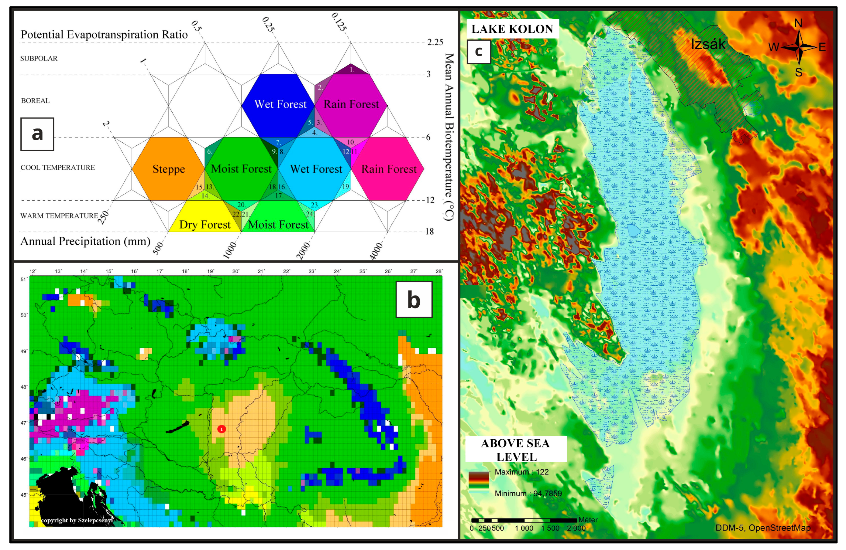
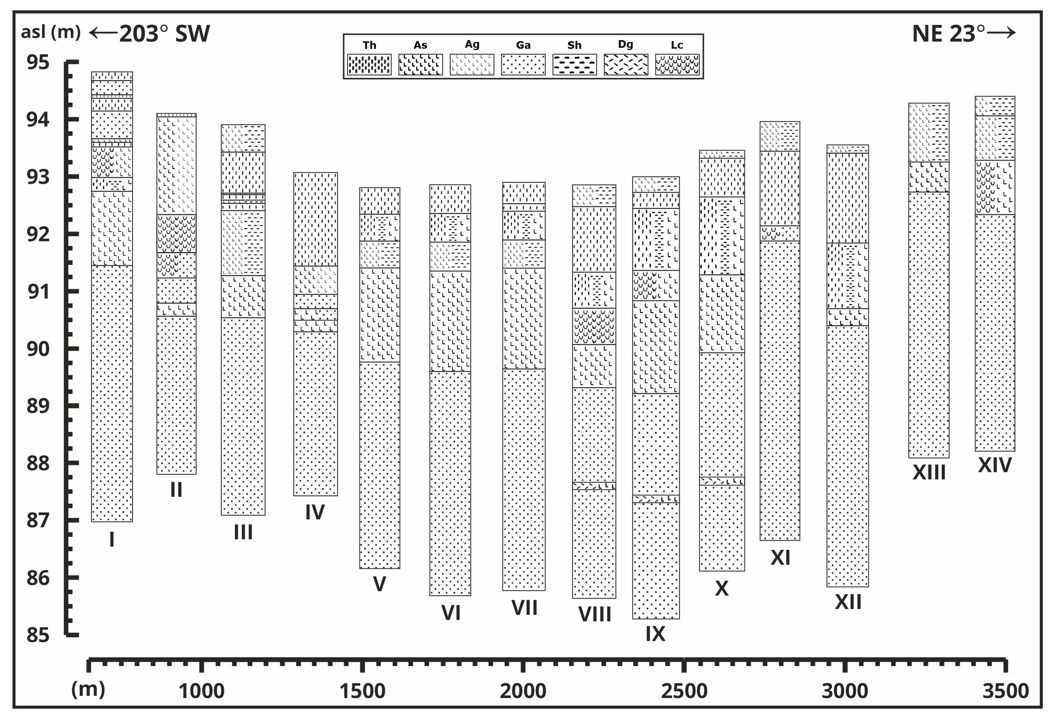
Lake Kolon can be found in the center part of the modern, unusually wide woodland–grassland ecotone, Pannonian forest–steppe region (Figure 1a,b) which covers an area of ca. 100,000 km2 nestled in the heart of the Carpathian Basin [1]. A geochemical and sedimentological section with PCA analyses has already been presented earlier [2] as there was no opportunity to collectively present the changes in various factors within the framework of a single article, due to reasons of scope. Pollen, macrobotanical and malacological data were analyzed earlier as well [3,4], but in this article, we aim to extend the statistical analyses of the species from the available data and pair the results with the newly modeled radiocarbon ages [2] to reconstruct more precisely the paleoenvironmental and vegetational changes that occurred from the end of the Last Glacial Maximum (LGM) in the center of the Great Hungarian Plain. As the development, timing, and formation process of the Pannonian forest–steppe are of utmost importance [5,6], a geological cross-section is established within the sedimentary basin. Within these cross-sections (Figure 2), the deepest, well-watered, and well-covered area was selected (VIII) for analyses in previous studies [2,3,4], and also mainly in this article. In addition to the environmental aspects, the research also delves into the historical context of the area from the Middle Ages. This historical perspective is not only valuable for historians and archaeologists interested in the region’s human history and land use practices, but also gives information about the history of the flora, fauna, and geology and the changes they went through due to constant anthropogenic influence.
Study Area
Lake Kolon is one of the most renowned lacustrine-marsh sedimentary accumulation areas in our region (Figure 1c). A description can be traced back to as early as 1055 AD, appearing in the first historical documents in Latin (with Hungarian words) in the foundation charter of the Tihany Abbey [12]. Today, it is a filling marshland interspersed with bog patches, which have developed within an abandoned Danube riverbed [3,4,13,14]. The undisturbed core (N: 46°46′12.85″; E: 19°20′43.47″) revealed pollen, macrobotanical, and malacological records within a depression covered by sandy skeletal soils (WRB: Arenosols) amidst sand dunes (Figure 1c), at the periphery of a fluvial alluvial cone developed during the Ice Age, and within the centre of Pannonian forest–steppe vegetation [3,4] (Figure 1a,b). Its current surface area is approximately 30 km2, but it was significantly larger (about twice) before the groundwater regulation in 1929. Sand dunes are found along the western edge of the lake, whereas sandy loess plateaus have formed along its eastern edges (Figure 1c). The marshy lake, speckled with lacustrine patches, is a 1.5–4 km wide belt extending longitudinally in a north-south direction within the dry terrestrial environment, consisting entirely of decomposed and original peat sediments [2,3,4].
The shallow lacustrine-marsh system of Lake Kolon is predominantly covered by reed beds (Phragmitetalia). In addition to Phragmites australis, other plants such as Typha latifolia, Typha angustifolia, Sparganium erectum, and Alisma plantago-aquatica are prevalent within the reed beds [15,16,17,18]. Orchidaceae species of outstanding significance and remnants of hardwood gallery forests are known on the marshy, wetland-covered periphery of the lake [3,4,19,20,21]. The lake and its surrounding area are known for their remarkable avifauna, despite being characterized by human activities such as grazing, haymaking, and reed harvesting. The entire region is protected and is a part of the Little Cumanian National Park (Kiskunsági Nemzeti Park).
The climatic conditions of the area, as depicted in the Walter-Lieth diagram [2], are characteristic of forest–steppe regions [7,8,9,10,11]. The annual (2011–2022) average temperature is 12.1 °C, and the annual (2011–2022) precipitation reaches 514 mm [2]. Based on recent climate data, the development of forest–steppe vegetation in the central Great Hungarian Plain appears to be climate-driven. However, the precise timing and manner of the development of the Pannonian forest–steppe remain uncertain. In our coring efforts, we have undertaken palaeoecological investigations to shed light on this matter.
2. Materials and Methods
Double overlapping undisturbed cores were retrieved using a 5 cm diameter Russian corer [22,23,24] from the lake [2,3,4,25]. The sedimentological characterizations of the cross-section cores (Figure 2) were conducted in accordance with the methodology outlined by Troels-Smith [26].
Figure 2.
Geological cross-section of multiple core sequences with Troels-Smith symbols [26].
Figure 2.
Geological cross-section of multiple core sequences with Troels-Smith symbols [26].

A core sequence (Figure 2(VIII)) was extracted from the basin’s deepest section, which was analyzed in previous studies [2,3,4]. Pollen (2 cm sample interval), plant macrofossil and malacological (4 cm sample interval) data [3,4] were employed with the newly modeled radiocarbon dates [2] and new statistical analyses to clarify the circumstances and evolution of Lake Kolon’s environment. Calibrated ages used in this article represent the precise geochronological results of Vári et al. [2], which is based on the raw radiocarbon data from Sümegi et al. [3,4]. Statistical analysis was performed by using PAST 3 Paleontological Data Analysis software [27]. Principal Component Analysis (PCA) was used to identify the main factors that control elemental distribution in the core section. Detrended Correspondence Analysis (DCA) was used to find the main factors and gradients that typify ecological community data. Before analysis, all pollen, malacological, and macrobotanical data were converted to Z-scores calculated as (Xi − Xavg)/Xstd, where Xi is the variable and Xavg and Xstd are the series average and standard deviation, respectively, of the variable Xi [25,28].
3. Results
3.1. Cross-Sections
The previously and currently analyzed [2,3,4] core is the VIIIth core sequence from the middle of the lake. Based on the cross-sections (Figure 2), the lower part of the section contains wind-blown sand everywhere, several meters thick. In three sections, the lower wind-blown sand layer contains fossil soils, closely adjacent to each other. In most sections, thick oligotrophic lake sediment accumulates on top of sediments deposited during and before the Last Glacial Maximum (LGM). The carbonate-rich mesotrophic lake phase (Chara-lake) is not universally present, and its thickness varies, and there are sections where it is very close to the surface. The eutrophic lake phase, marked by the beginning of peat sedimentation, produced relatively low organic matter content (around 30% max) [2] and served as a foundation to future peat accumulation. The extensive peat lake phase sediment is quite thick in some sections and often occurs near the surface, meaning the amount of peat decay and soil degradation was less and the anthropogenic effect was minimal or non-existent at that particular area. Additionally, beneath the surface-decomposed peat layer, smaller or larger peat layers are frequently found. In some areas of the lake, the formation and accumulation of very young peat can be assumed. These layers are less extensive and thick. Some of the sections located at higher topographical positions are characterized by mixed sediment layers near the surface due to the exposure to surface forming processes.
3.2. Pollen Analysis
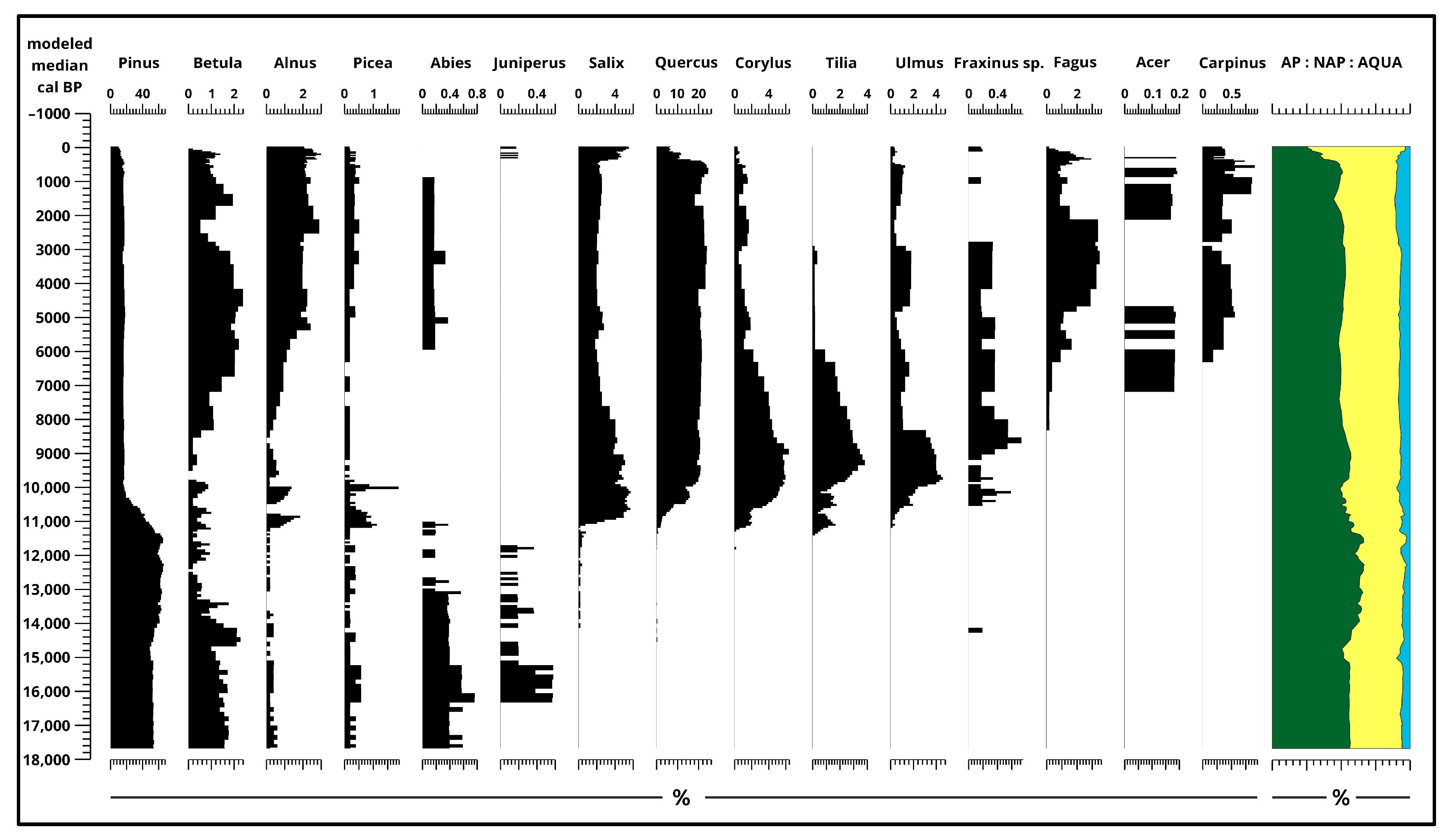
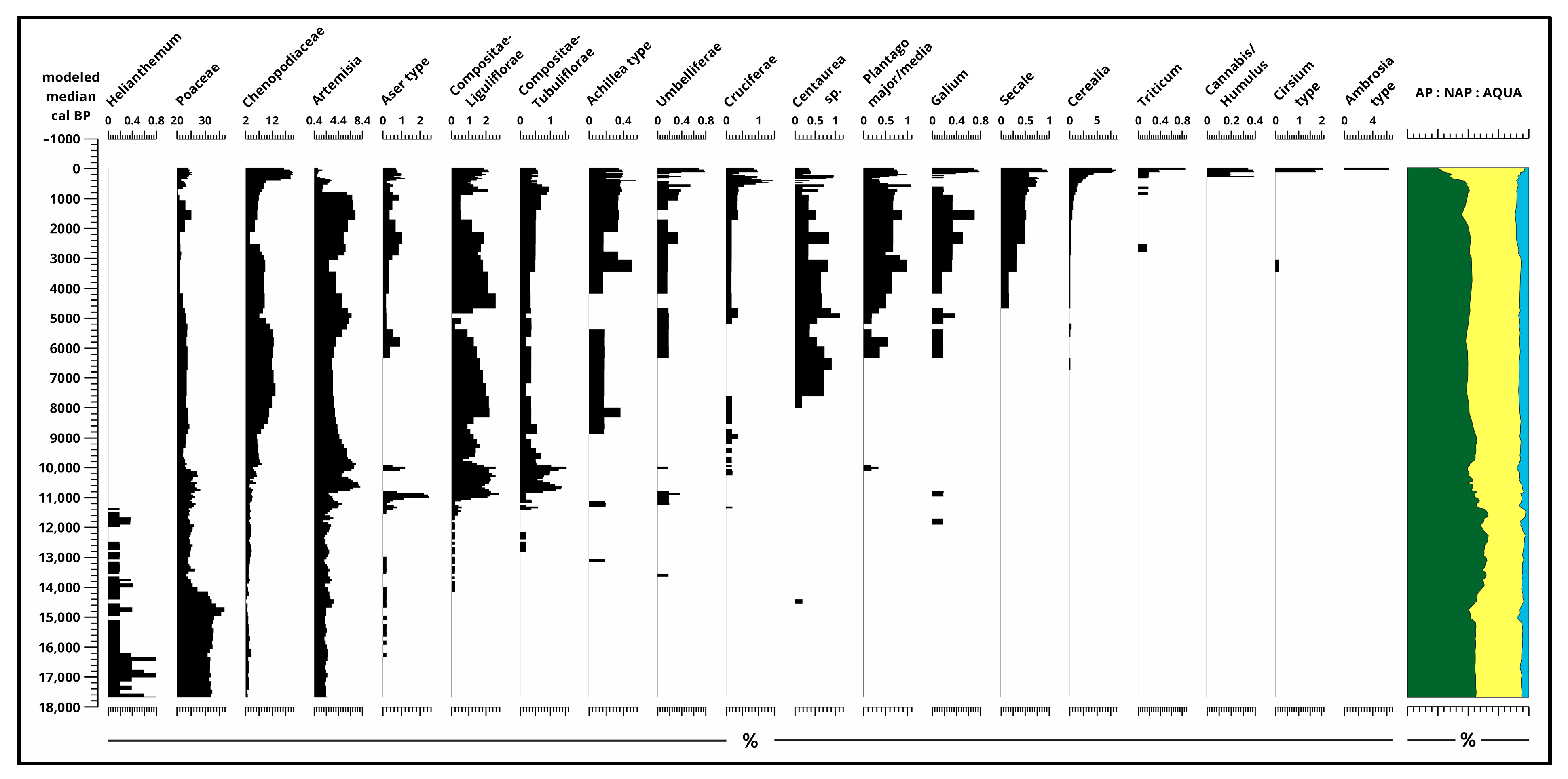
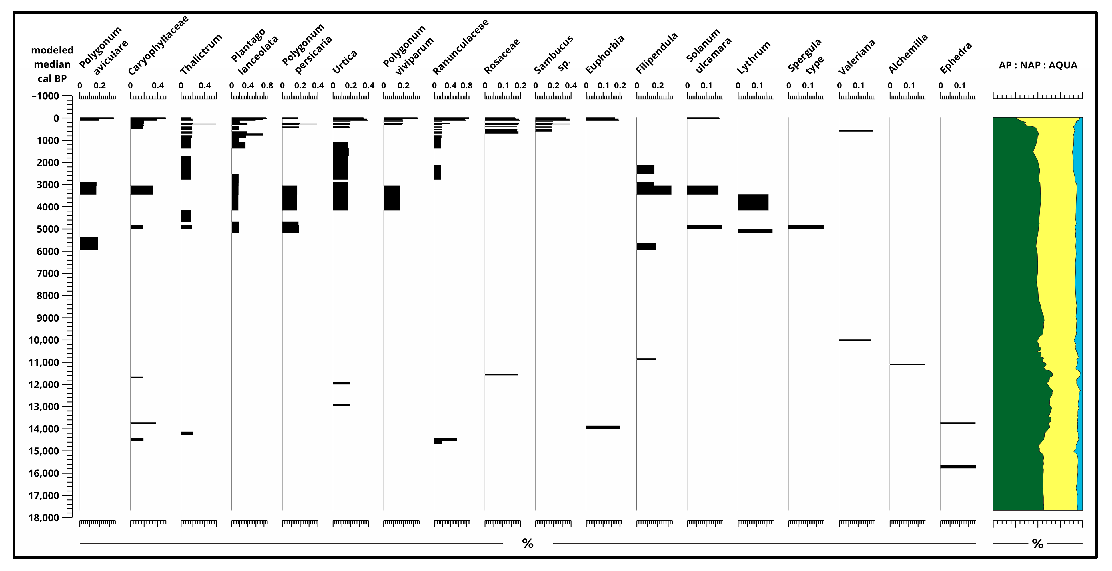
Based on the pollen data (Figure 3, Figure 4, Figure 5 and Figure 6 and Figures S1–S5), approximate changes in pollen composition can be observed dating back to around 17,700 years ago. Between 17,700 and 15,000 years ago, the ratio of Non-Arbor Pollen (NAP) to Arbor Pollen (AP) fluctuated between 40% and 60%. Then, between 15,000 and 13,000 years ago, the AP ratio notably decreased by approximately 10%, while the NAP ratio increased by the same amount. The proportion of aquatic (AQUA SUM) pollen and spores (Figure 6) remained consistently low throughout, only exceeding 5% in the last 12,000 to 10,000 years.
The composition of pollen between 17,700–13,700 years ago Pinus (53–60%), Poaceae (30–32%), Chenopodiaceae (2–4%), Artemisia (2–3%), and Betula (1–2%). Alnus, Picea, Juniperus, Helianthemum was present consistently but below 1%. From 13,700 years ago, the pollen composition in the Kolon Lake section was characterized by a predominance of Pinus diploxylon (60–65%) pollen until 11,400 years ago (160 cm) (Figure 3 and Supplementary Materials Figure S1).
The slow and gradual decrease in Pinus continues up to the surface, ending at 10%. Subsequently, from around 11,000 years ago (150 cm), deciduous trees, particularly Salix, Quercus, Corylus, Tilia, Ulmus, and Fraxinus, became dominant. Some NAP taxa (Figure 4 and Figure 5) also appear in this horizon, where Compositae, Liguliflorae, and Tubuliflorae reached their peak. The dominance of Corylus, Tilia, Ulmus, and Fraxinus was short-lived and while Corylus and Ulmus stayed present at around 1%, Fraxinus has only a few pollen remains in the top 60 cm, meanwhile, Tilia disappeared. With their decrease, in the later stages of the Holocene (around 80 cm) three new taxa appeared, namely Fagus, Acer, and Carpinus; meanwhile, Betula and Alnus also increased along with a small Abies presence.
Starting from the Middle Ages, tree pollen declined significantly, dropping below 30%. Consequently, during the Middle Ages, pastures were established, which became the most important agricultural use of the area from the second half of the Middle Ages.
The proportion of Non-Arbor Pollen has been significant since the end of the Ice Age, although it is not possible to determine specific taxa at the species level. However, even before the development of Neolithic farming [29], at the beginning of the Holocene, between 11,000 and 12,000 calibrated years ago, herbaceous elements typical of western European weedy vegetation [30] were present and made up a significant portion of the pollen assemblage over the past 17,700 years. Cultivated plants, especially cereal pollen (Figure 4, Figure 5 and Figures S2 and S3), appeared in large quantities primarily during the second half of the Holocene, starting from the Bronze Age. Their first appearance in the examined section dates back to the end of the Neolithic period.
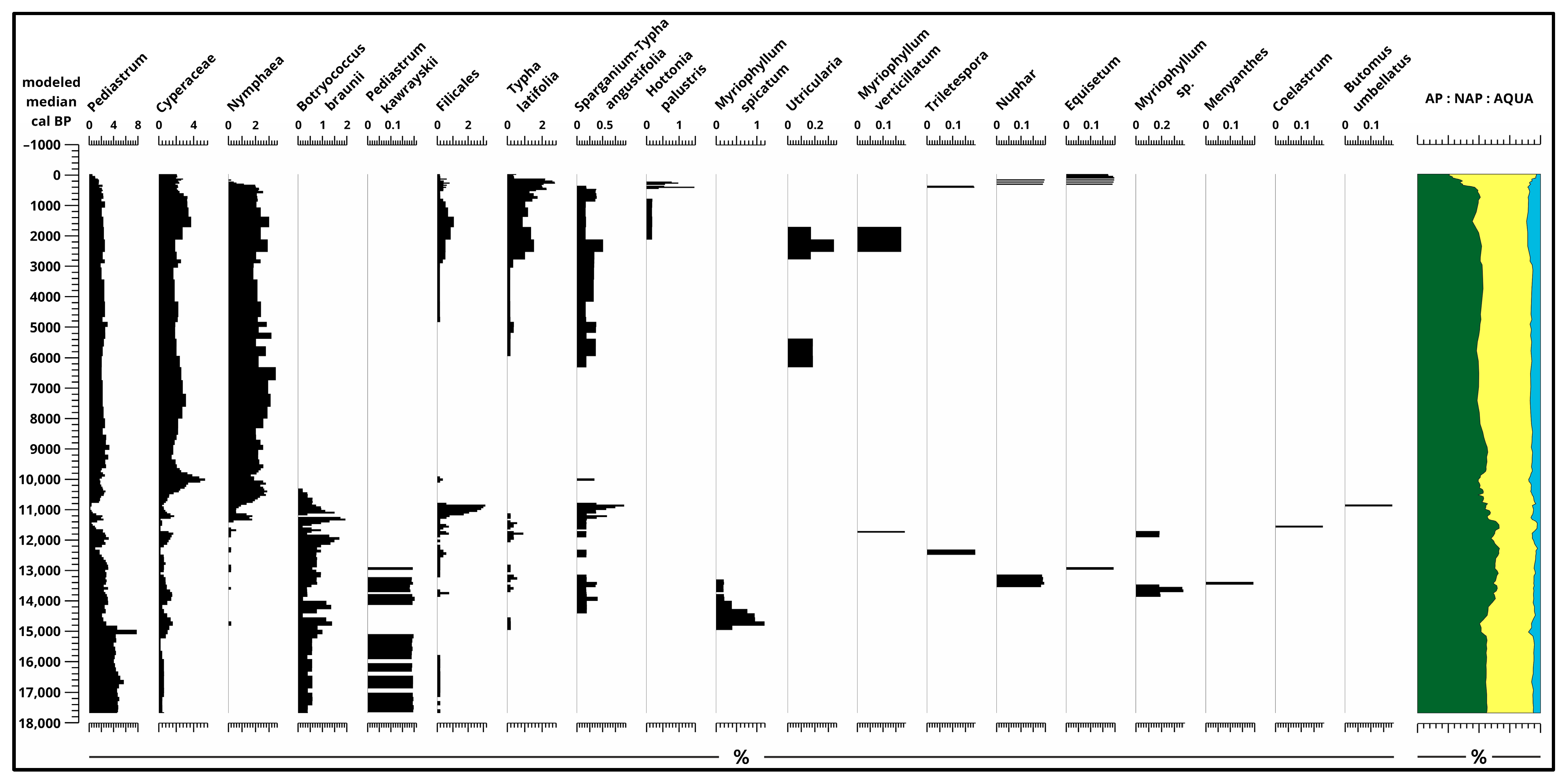
Remains from aquatic (AQUA) taxa (Figure 6 and Figures S4 and S5) are between 5–10% in the whole sequence constantly, only dropping down to 2–3% in some samples and mainly near the surface. Pediastrum (ca. 1–8%) and Cyperaceae (ca. 0–5%) are present in the whole core sequence; meanwhile, Botryococcus braunii (120–280 cm, 0–2%) and Pediastrum kawrayskii (200–280 cm, 0–0.2%) can only be found in the bottom half of the sequence, along with a small one-time spike of Myriophyllum spicatum (210–240 cm, 0.2–1.5%). Nymphaea has a few remains between 170–240 cm (in 12 samples), but increases significantly after 160 cm. Filicales, Typha latifolia. and Sparganium-Typha angustifolia pollen was found between 140–230 cm and near the surface from ca. 70 cm.
3.3. Macrobotanical Analysis
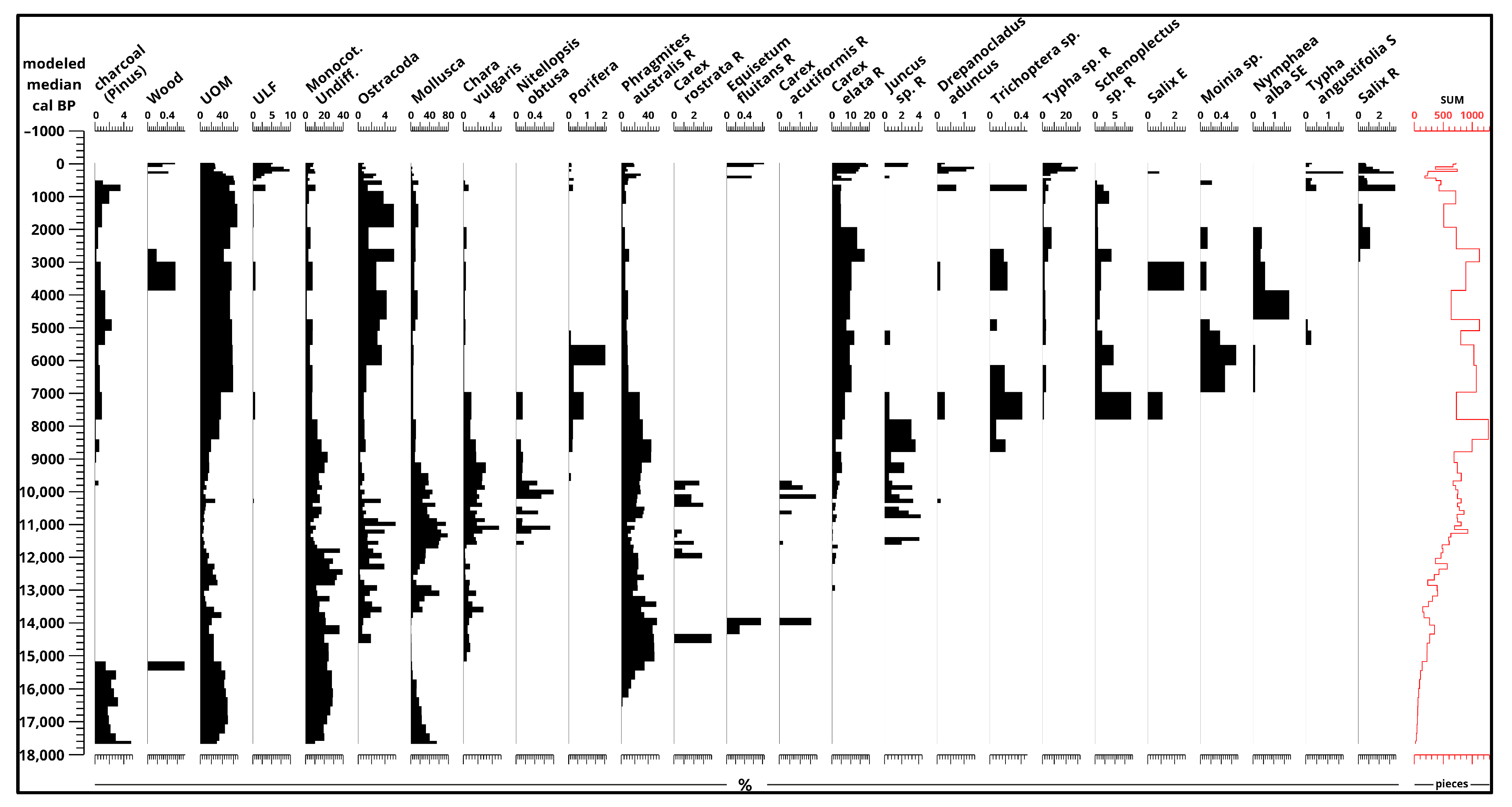
The macrobotanical remains at the end of the Ice Age were composed primarily of Pinus sylvestris and Betula nana tissue, as well as unidentified monocotyledonous remains (Figure 7). Then, at the beginning of the late glacial period, the remains of reeds (Phragmites australis) appeared, followed by the remains of sedges (Carex rostata and Carex acutiformis). The remains of Equisetum fluitans at the end of the Ice Age indicate that during this macrobotanical phase, a living water inflow characterized the Kolon Lake, likely from the Danube’s freshwater branches, and it may have been in an oligotrophic lake stage.
During the late glacial period, the appearance of reed, Chara, and Juncus remains was significant, leading to the development of a mesotrophic lake phase (Figure 7 and Figure S6). Based on the proportion of reed tissues, the lake’s depth may have been less than 2 m at this point, and the entire lake could have been covered with reeds.
In the present day (Holocene), macro remains became more abundant. Initially, Juncus, Carex, and Phragmites predominated, and as sedimentation progressed, Typha, Salix, and Nymphaea alba remains became more common. Both the macrobotanical remains and the Troels-Smith classifications [26] indicate the development of eutrophic lake conditions followed by marshy and swampy lake states from the beginning of the Holocene.
3.4. Malacological Analysis
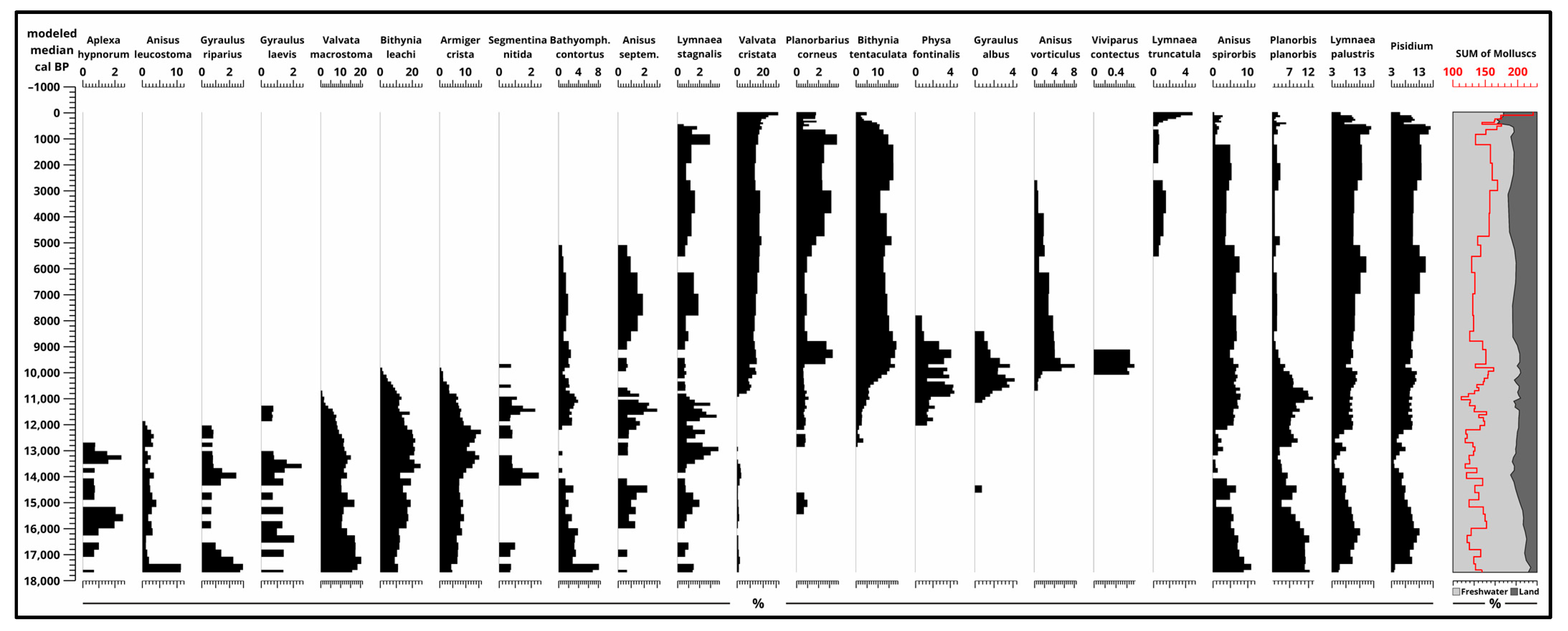
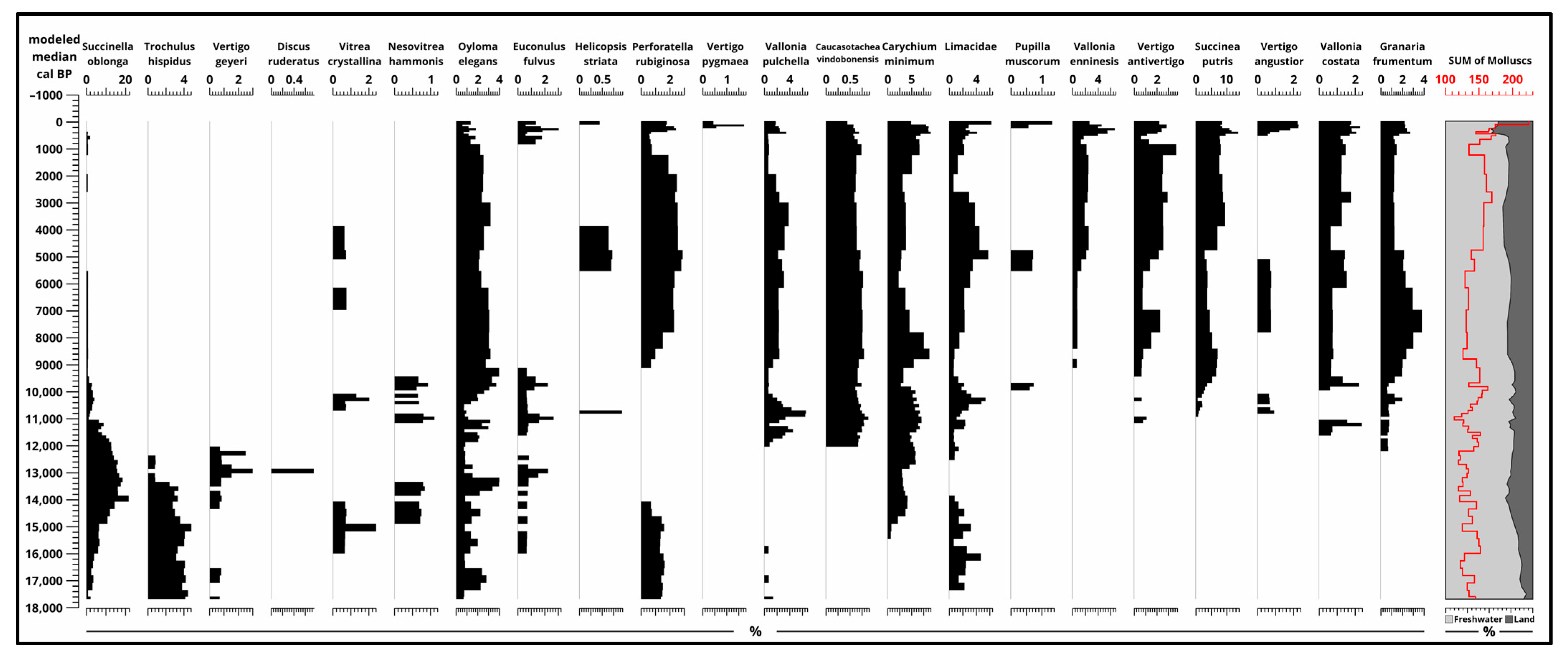
The dominance of freshwater species (Figure 8 and Figure S7) is present in all phases of the sequence. From the oligotrophic phase, terrestrial molluscs (Figure 9 and Figure S8) are gradually increasing from 10%, and they reach their maximum near the surface at 40%. This means that freshwater molluscs and mussels are between 60–90% in the sequence. Of these, Pisidium, Lymnaea palustris, Planorbis planorbis, and Anisus spirorbis are present during the whole sequence. Of the land molluscs, Oyloma elegans is present through all the sequence and a few other species like Succinella oblonga, Limacidae, and Carychium minimum are present with a small hiatus. It is important to keep in mind that the 4 cm sample interval does not enable the same resolution as other analyses with a 2 cm sample interval.
In the glacial portion of the section, cold-tolerant aquatic species that are no longer found in the Great Hungarian Plain [31] were present, including taxa like Valvata macrostomata, Bythinia leachi, Gyraulus riparius, and Anisus leucostoma. These taxa then declined, and more eutrophic-tolerant species, particularly Physa fontinalis, Bithynia tentaculata, Planorbis planorbis, and Anisus septemgyratus, became dominant. By the beginning of the Holocene, taxa such as Ansis vorticulus, Gyraulus albus, and Hippeutis complanatus had become dominant.
In the later part of the Holocene, species adapted to periodic drying and rich organic matter content in marshy and swampy lake environments, such as Valvata cristata and Lymnaea truncatula, dominated. Among the terrestrial species that emerged during the glacial stage, cold-resistant taxa capable of enduring cooler climates like higrophilous Succinella oblonga, Trochulus hispidus, Vertigo geyeri, and Discus ruderatus were found (Figure 8, Figure 9 and Figures S7 and S8). As the late glacial period progressed, cryophilous or cold-resistant taxa declined, and mesophilous species dominated during this time (Figure 8, Figure 9 and Figures S7 and S8).
At the beginning of the Holocene, species characteristic of Southeast European temperate forest–steppes, such as Caucasotachea vindobonensis, and those typical of open temperate steppes like Granaria frumentum appeared. As the riverbed filled during the Holocene, Limacidae, Vertigo antivertigo, Succinea putris, and Vallonia pulchella species became dominant. In the closing stage of the Holocene, the development of closed peat bog environments is indicated by the presence and proportion of species like Vertigo angustior, Perforatella rubigonosa, and Vallonia enniensis (Figure 8, Figure 9 and Figures S7 and S8).
3.5. Statistical Analysis
Principal Component Analysis (PCA) was performed on the pollen, malacological and macrobotanical results to reduce data dimensionality and identify the patterns of variation. The largest proportion of the variance (minimum 60%) in the data was explained usually by the first four principal components, making them the most informative for investigation and visualization. Detrended Correspondence Analysis (DCA) was performed on malacological (top 25 freshwater and terrestrial molluscs) results only.
3.5.1. Arbor Pollen
PC1 explains 40.09% of the variability and the taxa present and dominating the top half of the sequence in this component are: Quercus, Salix, Ulmus, Corylus, Fraxinus, Tilia, Alnus, Carpinus, Fagus, and Acer (Table 1). PC2 explains 22.88% of the variance and represents Carpinus, Alnus, Fagus, Betula, and Acer, taxa which are dominant near the surface. From the 15 different PCs, there was none where taxa that are present in the whole sequence from top to bottom (mainly Pinus, Betula, Alnus, Picea, and possibly Abies and Juniperus) are represented together in one PC.
3.5.2. Non-Arbor Pollen
Only the top 25 taxa were analyzed (Table 2). PC1 explains 51.06% and along with it represents a wide range of NAP taxa, understandably, with loadings ranging between 0.10–0.25. This component is connected mainly to the upper part of the sequence (0–160 cm). Taxa with negative loadings are Artemisia, Helianthemum, and Poaceae. PC2 explains 14.38% and represents Helianthemum, Poaceae and a few taxa with positive loadings from the upper part between 0–70 cm.
3.5.3. Aquatic Pollen
Six principal components described 61.81% of the variance, making the desired reduction in data variability less effective compared to cases where two, three or four components make up more than 60% of the variance (Table 3). PC1 explains 17.62% of the variance, is connected to the upper part of the sequence (0–160 cm) and primarily represents (loadings greater than 0.3) Cyperaceae, Nympaea, and Typha latifolia; meanwhile, the greatest negative loadings are Pediastrum, Pediastrum kawrayskii, and Botryococcus braunii. PC2 explains 11.98% of the variance, with Filicales, Butomus umbellatus, Sparganium-Typha angustifolia and Botryococcus braunii having great positive loadings. PC3 explains 10.41% of the variance and represents Nuphar, Hottonia palustris, Equisetum, and Typha latifolia. This component is also connected to the upper part of the sequence. PC4 explains 8.49% of the variance and two taxa, Myriophyllum verticillatum and Utricularia, are present with the greatest loadings, representing a small part of the whole section (around 50–76 cm). PC5 explains 7.21% of the variance and Trilete spore, along with Hottonia palustris, has high loadings for this component. Finally, PC6 explains 6.10% of the variance, making the cumulative variance to 61.81%. Manyanthes has the highest loadings for this component.
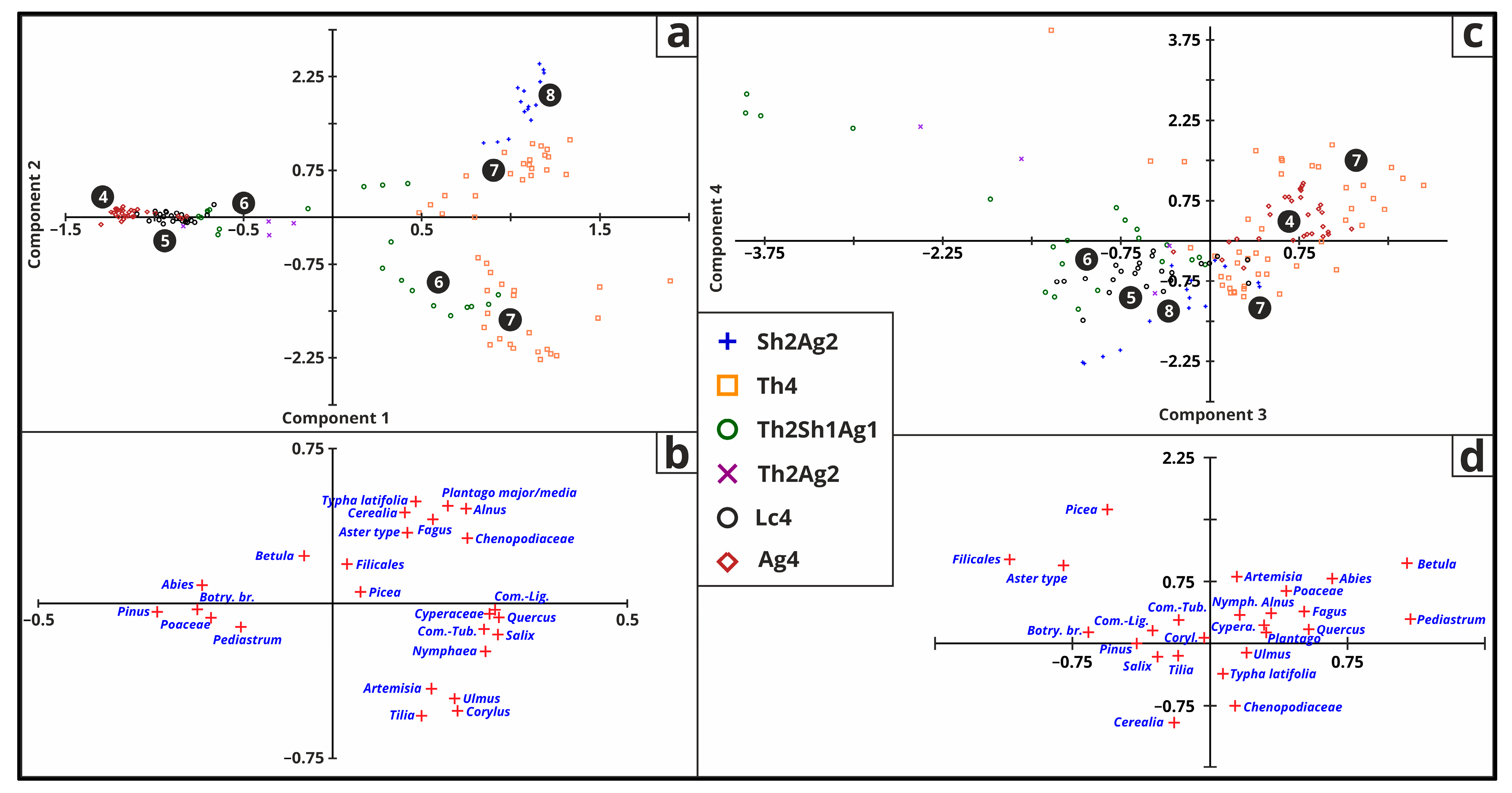
3.5.4. All Pollen
For this statistical analysis, the top 25 taxa were employed from both AP, NAP and AQUA pollen (Table 4, Figure 10). PC1 explains 41.29% of the variance and 10 different taxa has loadings greater than 0.2 for this component: Quercus, Salix, Cyperaceae, Nymphaea, both Compositae taxa, Chenopodiaceae, Alnus, Corylus, and Ulmus. This component describes the upper part of the sequence from 160 cm. PC2 explains 18.18% of the variance and taxa that are dominant in the top 70 cm are represented. PC3 explains 10.92% of the variance and mainly represents Pediastrum, Betula, Abies, Quercus, and Fagus. PC4 explains 7.95% of the variance and represents Picea, Filicales, Aster type, Betula, Artemisia, Abies, and Poaceae.
3.5.5. Malacology
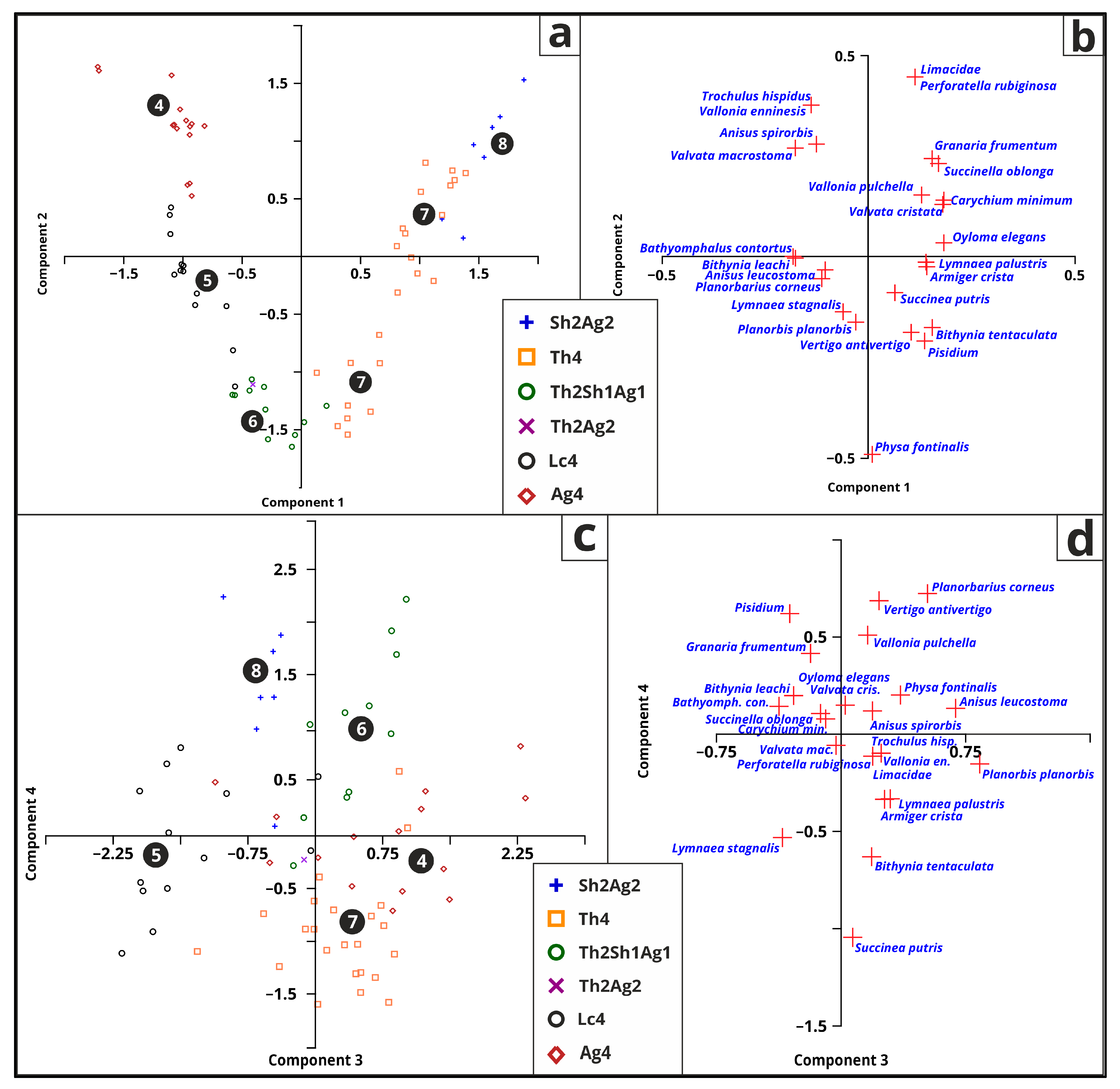
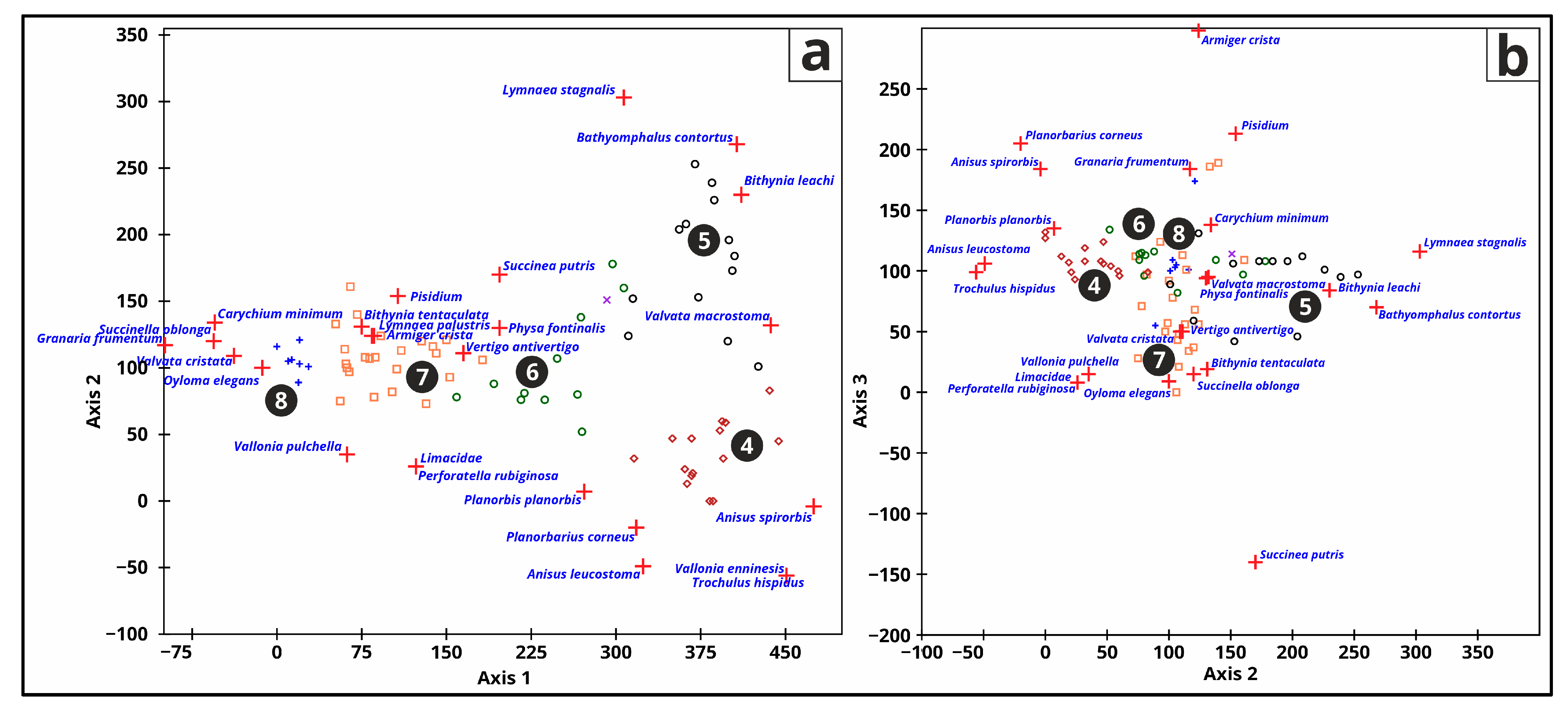
For this analysis, only the top 25 taxa were employed for PCA (Figure 11 and Table 5) and DCA (Figure 12). PC1 explains 45.07% of the variance and represents Oyloma elegans, Carychium minimum, Valvata cristata, Succinella oblonga, Bithynia tentaculata, Granaria frumentum, Armiger crista, and Lymnaea palustris. PC2 explains 15.04% of the variance and represents Perforatella rubiginosa, Limacidae, Trochulus hispidus, Vallonia enninesis, Anisus spirorbis, Valvata macrostoma, and Granaria frumentum. PC3 explains 11.40% of the variance and represents Planorbis planorbis (positive loading of 0.5203), Anisus leucostoma, Planorbarius corneus, and Physa fontinalis. PC4 explains 7.04% of the variance and represent Planorbarius corneus, Vertigo antivertigo, Pisidium, Vallonia pulchella, and Granaria frumentum. PC1 and PC2 in Figure 11 separate the Chara-lake and peatland phases, and species distributions can be observed.
The terrestrial and freshwater snail fauna fundamentally transformed with the emergence of various lake phases and the onset of environmental changes (Figure 12). Some terrestrial species only came after the eutrophication started and the lake changed from a mesotrophic Chara-lake. Freshwater snails constantly changed, overlapping each other. The distribution of lake phases is not as split as in the PCA analyses.
3.5.6. Macrofossil
For this analysis, only the top 25 data categories were employed (Figure 13 and Table 6). PC1 explains 22.80% of the variance and the greatest loadings are represented by Carex elata R, Unidentifiable Organic Matter (UOM), Typha sp., Salix R, Unidentifiable (ULF), Depanocladus aduncus, Schenoplectus sp. R, wood and Pinus charcoal. PC2 explains 15.81% of the variance and represents Ostracoda, Schenoplectus sp. R, Trichoptera sp., Moinia sp., Phragmites australis R, Porifera, Chara vulgaris, and UOM. PC3 explains 13.23% of the variance and represents Juncus sp. R, Phragmites australis R, Monocot. Undiff., Chara vulgaris, Typha sp. R, Drepanocladus aduncus, Nitellopsis obtuse, Equisetum fluitans R, Carex acutiformis R, and ULF. PC4 explains 7.25% of the variance and represents Moinia sp. and Porifera remains. PC5 explains 6.38% of the variance and represents Mollusca, Ostracoda, Carex rostrata R, Nitellopsis obtuse, Chara vulgaris, Drepanocladus aduncus, and Salix R.
4. Discussion
4.1. Paleoecological Changes
Overall, the average dominating (identified) taxa in the top 280 cm of the sequence for Arbor Pollen are Pinus, Quercus, Salix, Corylus, Tilia, and Ulmus; for Non-Arbor Pollen are Poaceae, Chenopodiaceae, Artemisia, and Cerealia; for Aquatic Pollen are Pediastrum, Cyperaceae, and Nymphaea; for freshwater are Valvata cristata, Bithynia leachi, Bithynia tentaculata, Valvata macrostoma, Lymnaea palustris, Pisidium, Anisus spirorbis, Anisus leucostoma, and Armiger crista; and for terrestrial molluscs are Succinea putris, Sucinella oblonga, Oyloma elegans, Perforatella rubiginosa, Carychium minimum, Granaria frumentum, and Vallonia pulchella. Main pollen dominance can be more easily described, and their changes can be tied to climatic changes or environmental changes (lake phases) than mollusc changes, where there is more overlapping between phases and species (4) that are present during the whole sequence.
The investigated profiles at Lake Kolon roughly span the changes of the past 17.7 thousand years [2], and the pollen, malacological, and macrobotanical studies are allowing the reconstruction of the vegetational and malacological changes [3,4] from the end of the Last Glacial Maximum (LGM) up to the end of the Holocene. Lake Kolon exhibits an exceptionally diverse development, from a sandy and loessy fluvial and aeolian [2] sediment deposition to peat formation with rich avian species and diverse vegetation. The historical records, results and cross-sections suggest that the lake was much larger, had simultaneously multiple small beds in different elevations and that these connected from time to time and stayed connected from shorter or longer intervals.
Based on the results and remains, a boreal taiga–steppe evolved in the area at the end of the LGM with tundra-like vegetational patches [3,4]. The freshwater malacofauna can be synchronized to the European loess zone that developed during the cold maximum in the Ice Age. The terrestrial malacofauna showed correlation with the malacofauna from the loess sequences from the Great Hungarian Plain from this interval, although the lake’s water surface strongly affected the local climate and fauna elements. During the LGM, in the Danube–Tisza Interfluve, an open parkland-type boreal forest–steppe dominated with 7–8 °C cooler summers than today [2,4]. Between ca. 17,700–15,000 cal BP (240–280 cm), a significant amount of Pinus charcoal was found, meaning that wild forest fires occurred after the LGM with the increasing temperatures that are also signaled by the summarized paleoecological results. Poaceae also stagnated in this interval and started to increase after 15,000 cal BP for a short period but declined in significance from 13,700 years ago. Betula also experienced a stagnation followed by a greater spike, after which it decreased.
After 15,000 cal BP, Pinus started to dominate (60–65%) for almost 4000 years, when the temperature started to change drastically in the Carpathian Basin and temperate forests started to rapidly spread. Between 13,700–11,700 cal BP (ca. 220–172 cm), during the mesotrophic Chara-lake phase, a really slow transformation into temperate forest–steppe vegetation occurred. Salix and Quercus had >1% values between ca. 15,000–11,000 cal BP (232–152 cm), and they started to first increase gradually, then had a huge increase, during which other temperate species showed up (Corylus, Tilia, and Ulmus). Based on the data, it appears that a relatively rich boreal forest–steppe fauna community in snail species transitioned into a relatively impoverished Holocene temperate forest–steppe fauna community during the Pleistocene/Holocene transitional phase. The changes occurred so concurrently and temporally in tandem that a clear relationship can be discerned among them, and as a result of these changes, it can be reconstructed that the forest–steppe structure was inherited, but in higher temperatures and drier microenvironments, elements that became prevalent during the Holocene period occupied various parts of the mosaic environmental structure. Although there are some studied species and taxa that are present during the whole sequence, flora and fauna diversity grows rapidly from 11,400 cal BP (160 cm), shortly after the peat accumulation and the Holocene started (11,700 cal BP).
The communities contributed to environmental change by reducing the woody cover of the forest–steppe region and established a cultural steppe. The natural temperate forest–steppe with deciduous trees that developed during the early Holocene underwent significant transformation due to human influence over the past approximately 8000 years, evolving into human-induced open parkland, a transition that had already begun during the Iron Age. Corylus and Ulmus decreased and Tilia disappeared along with Fraxinus; meanwhile, Betula and Alnus increased, Fagus, Acer, and Carpinus, along with Abies, appeared. Quercus and Salix stayed relevant with Pinus and with a small amount of Picea. Along with these changes, herbaceous changes occurred with emerging species like Aser type, Achillea, Umbelliferae, Cruciferae, Centaurea sp., Plantago major/media, Galium, Secale, Cerealia, Triticum, and in the past few hundred years, Cannabis/Humulus, Cirisium type, and Ambrosia type. Based on charcoal remains, it can be inferred that forest burning has not occurred in the immediate vicinity of the lake since the medieval period. Pastures became the most important agricultural use of the area from the second half of the Middle Ages.
4.2. Medieval History
Hungary’s first written relic is connected to Lake Kolon. Although the environmental history of the area has changed since the Neolithic period [2,3,4], it is clear from written sources [12] (the Tihany Founding Charter, 1055: DHA I; PRT X) that the environmental transformations accelerated during the reign of St. Stephen (997–1038) when the agricultural system of the Kingdom of Hungary was established. The portion of the Tihany Founding Charter related to this study area, translated from Latin, reads as follows: “There is a place for grazing horses, which begins at U[gr]in’s idol, from here to a valley, then to a dune, then to pre-sand, then to three lakes, then to a fox hole, then to three mountains, then to Iohtucou, then to the sands of Báb, then to the place of Alap, then to Kövesd, then from the middle of the water called Kolon to the fekete humuc, then to fuegnes humuc, then to cues humuc, then to Gunasara, then all the way to Szakadát and then to Sernyehalom, then to a ditch which goes all the way to the idol” [12]. The former Kolon praedium (estate, property) was donated by King Andrew I of Hungary (ruling 1046–1060) to the Tihany Benedictine Abbey in 1055 (Figure 14). The tour of the border is a medieval legal practice, a field inspection, that was carried out by recording the natural or artificial boundary points of an estate, estate part or settlement [32,33].
From the perspective of Lake Kolon, those areas and boundary markers are of outstanding significance that in their naming—in most cases as a suffix of a compound word—the term sand (homok, humuc(h), humuk, homoka) or its Latin equivalents (arena, sabulum) are mentioned, which presumably refers to the material of the area [34]. A good example of this is the sandy boundary area mentioned in the deeds (e.g., terra sabulosa vel arenosa), the name of a wasteland/settlement (e.g., sabulum Bab = sands of Báb, [35,36]) or the mention of a sand dune (e.g., Sernyehalom [37]). Significant information about the geographical conditions can be gained by further analyzing place names. Thus, with their help, some types of sandy soil can be identified (English/Hungarian/Old Hungarian: black sand—fekete homok—fekete humuc, rocky sand—köves homok—cues humuc, peaty sand—fövenyes homok—fuegnes humuc).
According to the identification of historian György Györffy (1917–2000), the area covers the present-day border of the town of Izsák, and his studies and opinion suggest that a large part of the borders are in agreement with the current borders [38]. From the Latin description, it is clear that on the Kolon praedium, the stablemen of the Tihany Abbey lived; that is, the estate may have been of a livestock-raising nature [39]. Prior to their direct capture and shaping into riding horses, three and four-year-old colts were raised (harmadfű and negyedfű, which literally means thirdgrass and fourthgrass, is said about foals and young cattle, which are already entering their third or fourth year of age, that is, they step out onto the fourth new grass), grazed, and they ran them (due to mosquitoes, they had to move, gallop, and train) on the meadows around the marshy strip of Lake Kolon. Geographically, the accurate description of the sand dunes and the presence and mention of the marshes and lakes (semlyék, semlyékek in plural form), is mostly used between the Danube and Tisza area and is a wet, periodically covered shallow depression, meadow, brackish, watery area, wind furrow, and in another interpretation, plant sediment washed into a lump by water [40,41,42,43] is interesting in the 11th century founding charter.
In more detail, the 1211 charter that confirms the abbey’s property rights speaks of the lake itself [38,44]. The descriptions and analysis reveal to us the image of the former Kolon praedium (Figure 14). The area exhibits the characteristic landscape of the Kiskunság region, featuring sand dunes, the shallow depressions between them (semlyékek [40,41,42]), flat meadows, marshes, natural vegetation, as well as ditches, settlements and roads. The presence of the conquering Hungarians in the area may be indicated by the burial sites containing partial, palmette-decorated horse saddles from Soltszentimre and Izsák-Balázspuszta, suggesting that the area may have been a prominent settlement site for them [45]. Later, permanent settlements, which still exist today (Izsák, Páhi, Soltszentimre [originally Pusztaszentimre], Csengőd, Akasztó), developed around the lake [46], and their churches were typically built from locally sourced meadow limestone.
Given that the utilization of the landscape and the economic utilization of a particular area are closely intertwined with the former soil and its quality, the investigation of the type of sandy soils in this case can provide important information for the study of the history and environmental history of the medieval Lake Kolon and the surrounding Homokhátság region. However, the research on medieval soil types is not an easy task, partly due to the lack of systematic research and the limited opportunities provided by written sources. Furthermore, the study of mediaeval soil types is even more complex as contemporary maps cannot be relied on, and instead, the mention of border inspections in the charters must be relied upon. An important reference point for the analysis is the terminology used in the classification of soils in Hungary, as in some cases it is possible to compare the modern terms used for soil types [40,41,42,47,48,49,50,51] with the terminology translated from medieval Latin.
The 1211 land survey (before the Mongol invasion of Hungary, which occurred between March 1241 AD and April 1242 AD) conducted at the Lake Kolon property provides detailed information about the mediaeval agricultural environment, as the property was thoroughly surveyed over several days (Figure 14). The size of the praedium is indicated by the fact that it took approximately three days to cover 40 km on horseback and foot, discussing and recording the boundaries. Approximately one-third of the survey focused on the Lake Kolon area and its surroundings, while a smaller amount, one-fourth, covered the meadows and their surroundings of Orgovány and Ágasegyház. One of the significant values of both the 1055 and 1211 land surveys is that both started from a point called Bálvány (1055: baluuana, 1211: Balanus), and then proceeded south, then west (going around Lake Kolon) and finally east [12,38].
The Kolon Lake is now a nature reserve, but its development history is also closely related to the changes in the land in the 11–13th centuries after Christ. The 1055 charter [12] (Figure 14) distinguished three types of sand on the western shore of the lake, in the Bikatorok sand dune area: black sand—fekete homok—fekete humuc, rocky sand—köves homok—cues humuc, and peaty sand—fövenyes homok—fuegnes humuc. The term fekete humuc probably referred to the dark-colored sandy slime that formed on the periodically wet and dark-colored algal mat on the shore of the lake, or the dark-colored sandy slime that formed in the intermediate zone between the two dry running sands (bucka—mound) that make up the dune [52]. The term fuegnes humuc probably referred to the darker, peaty, more humus-rich sands that were located west of the black sands and likely belonged to the highest dune range in the area, which rose 120 m above sea level [12,38]. This provided an extraordinary opportunity for spatial identification in the 1211 property survey, as it also separated sand hills (ad monem sabulosum). The term cues humuc probably referred to the diagenetic and cemented sand fragments and pebbles that were formed as a result of the influence of the limey and alkaline groundwater in the Reveckei-halom dune formation. Probably the modern Reveckei-halom can be identified with the Cuest (Köves) dune of the 1211 charter. The shape of the dunes belonging to the Lake Kolon is well reflected in the term mont iculus (small hill, small mound), as this term well describes the longitudinal mounds that stand out 10–20 m from their environment and are characterised by steep edges [53]. In the 1055 charter, the SW border of the Kolon estate is referred to as Gunusara (Gönyüs ár), which hypothetically can be identified as a lower-lying, periodically flooded meadow on the western shore of the lake. In the 1055 boundary survey, the term aqua (water) is used in relation to Lake Kolon, which clearly indicates an open water surface [12,54]. The 1211 charter uses the term as tagnum (smaller still water, lake) four times and with the mention of rippa (shore, water front, waterside) clearly indicates that in the 13th century, the Kolon system also appeared as a lake (Figure 14). Therefore, it is questionable to describe Lake Kolon as a marsh [38], rather it is more likely to be a stable water surface with significant vegetation (eutrophic lake) [55].
The 1055 and 1211 property inspections (Figure 14) provided us with the opportunity to reconstruct the vegetation along the shore of the lake [56,57] (Figure 14). The 1055 property inspection referred to the Kulun (Kolon) praedium as “est locus ad pascua equorum” (a place for horse grazing) [12,54]. This is also supported by the etymology of the name Lake Kolon, as it is likely to have originated from the Old Turkic word qulun (foal). Grasses (Poaceae), such as various Festuca (csenkesz) and Poa (perje) species, and the Stipa (árvalányhaj) taxon are suitable for horse grazing. Based on pollen analysis [3], these herbaceous taxa are likely to have been present in large quantities in the terrestrial environment around Lake Kolon during the Middle Ages. The 1211 document also confirms the significant presence of grasses, as a territory was referred to as “dús füvű völgy” (a lush meadow valley) in the border description, while the expression ad campus (to the field) was mentioned on the eastern side of the lake. In addition, the 1211 property inspection used the terms pinus or feuneus five times. Both expressions can be associated with the presence of Juniperus communis (common juniper, boróka), a pine species that still exists in the region around Lake Kolon [58]. The final sentence of the 1055 founding property document “haec loca, quicquid in sefrutectis, in arundinet is, in pratis continent” (this land, with all its shrubbery, reeds, and meadows), provided significant help in reconstructing the mediaeval vegetation, as it clearly indicated that the surface of Lake Kolon was likely covered by reeds and the periphery by meadows. Radiocarbon dated palaeobotanical data also clearly support this [2,3,4]. The reconstructed image, based on the property inspections, suggests that larger and more continuous forests, which are present today (although some of them are artificial) in the environment of Lake Kolon, may have been absent during the Middle Ages—mainly based on the analysis of documents and certificates [58]. Therefore, in the Middle Ages, the open vegetation, which was influenced by human activity, may have dominated the area instead of the forest–steppe environment that is observable today, particularly on the southern side of Lake Kolon, near the Páhi settlement, where mixed oak–hornbeam–sycamore forests (Fraxino pannonicae—Ulmetum) can be observed today [15,16]. However, it cannot be ruled out that these forests did not belong to the praedium [44].
Certificates provided opportunities for the reconstruction of mediaeval settlements existing around the lake, which had formed prior to the destruction of the Ottoman Conquest in the late Middle Ages and early modern period [59]. The Hungarian village of Kolon, which was inhabited by 32 families, including 82 male family members, according to data from the 1055 property survey, emerged at the end of the Hungarian Conquest in the place where the city of Izsák is today [38]. Similarly, the border survey of 1211 recorded 4 serfs, 13 stablemen and 22 servants living in the same area [38,60]. Kolon village had its own temple dedicated to the worship of the Holy Cross. The villa Herbon (Herbon village), located on the eastern shore of Lake Kolon, a few kilometers from the lake, probably stood on the modern territory of the village of Orgovány, which is located on the Orgovány-bog shore [61]. It is believed that the area was originally a noble estate belonging to the Csák family, and one of its members was named Herbon. Based on this, it can be assumed that the area was a secular (noble) property, and it came under the control of the Cumans in the late Middle Ages as a secular property. Additionally, the presence of a location named “Vár Fehére” (the white of the castle) near Herbon village suggests that a portion of the land in the village was also held by the (Transdanubian) Fehérvár Church. The village of Herbon (after it was excluded from the property of the Csák family) was named Szentmária after the patron saint of their church in 1359 [62,63]. It is noteworthy that the area around Lake Kolon underwent significant changes during and after the first Mongol invasion of Hungary, with the settlement of the Cumans and the development of a network of new settlements around the lake in the 15th century [56,57,62]. This network of settlements was again transformed during the Ottoman conquest. As a result, the mediaeval settlement pattern underwent multiple transformations over the centuries and can only be reconstructed through archaeological excavations [58]. Therefore, environmental analyses based on material examination and dating provide a more reliable foundation for determining the development of the area, including the vegetation, than written sources, which are limited in their usefulness due to interpretational and locational problems, as well as their limited temporal applicability [63].
4.3. XX. Century History
Until the early 20th century, Lake Kolon had intermittent natural connections to the Nádas-rét near Szabadszállás to the north, primarily during periods of extremely high water levels. These connections were disrupted after the construction of the Kecskemét-Fülöpszállás railway in 1895 and the Kecskemét-Dunaföldvár main road in 1939 [64].
In 1912, the Pest County Drainage and Irrigation Association initiated the construction of the Danube Valley main canal, a 107 km long canal, to regulate the marshy Danube Valley and increase arable land. This led to the draining of Lake Kolon’s standing waters in 1927–1928 [65]. The drained lakebed showed signs of deterioration, with salty pastures, brackish ponds, shifting sand dunes, and reedy strips around its perimeter [66]. Agricultural experiments were attempted but proved unsuccessful due to poor soil conditions. The decrease in water levels had detrimental effects on traditional land use, including vineyards, orchards, meadows, pastures, and fishing, leading to a decline in these sectors. In the 1930s, the Hungarian Royal Geological Institute identified obstacles to Lake Kolon’s restoration, concluding that the lakebed was only suitable for grassland agriculture. Neglected maintenance of canals and other factors resulted in the return of reeds and marshes in the 1950s.
In 1955, the Budapest Irrigation and Soil Improvement Company proposed a land improvement plan emphasizing grassland farming and forest planting, but it was never implemented. Agricultural use of Lake Kolon was eventually abandoned. Peat subsidence and fires significantly altered the peat layer on the lake’s surface between 1931 and 1955. Large-scale peat mining began in 1952 but ceased in 1959 due to various challenges [64].
Lake Kolon had once served as a natural regulator of groundwater levels and flood storage, but this function was lost with the construction of the XV. Canal and its branches. Flood control plans began in the 1950s, but it was not until the flood year of 1965 that Lake Kolon’s deterioration prompted the construction of a reservoir system. A study by Miklós Bosznay in 1966 led to the acceptance and implementation of the reservoir system, with a combined storage capacity of 20.57 million m3 [64].
4.4. Rehabilitation
The first large-scale aquatic habitat rehabilitation in the National Park, aimed at providing shelter for the lake’s unique fish population during dry years, was executed at Öreg-víz between 1988–1989. The rehabilitation involved excavating nearly six hectares of open water to a depth of 1.5 m with Dutch support, but shallow water areas were not established at first. Since 2015, the transitional edge zones have been improved to address these deficiencies, allowing fish to reproduce in the easily heated shallow waters in spring. The first otter family also settled in the lake [66].
A mosaic wetland habitat rehabilitation in the northern part of a lake at Tókás was created based on previous conservation experience in 2010 [66]. It consists of 12 small ponds connected by channels and transitional zones between water surfaces and reed beds. The area is diverse and provides habitat for many plants, insects, and birds. Channels are difficult to navigate due to the common bladderwort (Utricularia vulgaris) that blooms massively in them. The inner part of the area near Izsák is not accessible but provides habitat for birds.
A large water surface area, Nagy-víz, was created between 2011–2013 because there were no natural open water surfaces in the 1400-hectare wetlands of Lake Kolon and artificial water surfaces were minimal compared to reed beds. This was carried out based on the findings of Sümegi et al. [3]. The 20-hectare open water, with varying depths of 1–1.8 m, is partitioned by islands to prevent strong waves and provide bird resting places. Shallow waters around the deep waters were created by cutting green reeds instead of dredging. The lake centre attracts many birds during breeding and migration, and rehabilitation efforts have introduced new species to the area. Additionally, a landfill with 16 shrub and tree species has been recultivated in the area and is expected to resemble a natural forest by the mid-century [66]. The area is freely accessible as part of the Bikatorok trail (Figure 15).
On the western side of the lake, remnants of sand dunes can be found, which were cleared and replanted with non-native pine and acacia trees. The sand dunes around Bikatorok are highly endangered due to the proliferation of non-native invasive species in recent decades, such as acacia and silky wormwood. The planned and intensive rehabilitation of the sand grasslands began in 2011 with the goal of reducing the proliferation of invasive species [66]. By 2013, more than 400 hectares of these harmful species had been eradicated, but since there are still many infection foci outside the protected area, ongoing work is needed to maintain the favorable condition of the grasslands. The rehabilitation of sand grasslands is a slow process that can take decades. However, the emergence of protected plant species is promising.
5. Conclusions
The research utilizes an interdisciplinary approach, combining geological, ecological, and historical methods with a focus on the development process of Lake Kolon. This information is not only valuable for understanding the past but also for informing present-day ecosystem management and conservation efforts in the region, providing critical insights into the dynamics of woodland–grassland ecotones, which are ecologically important transition zones.
It is evident that although a cross-sectional sequence summarizing several lake phases and environmental changes are observed, the geomorphology and the extent of the different lake phases greatly influence the development history deduced from a single section. The lake was previously much larger, had simultaneously multiple small beds in different elevations and that these connected from time to time and stayed connected from shorter or longer intervals.
The findings indicate the emergence of a boreal taiga–steppe ecosystem at the end of the Last Glacial Maximum, characterised by tundra-like patches. The lake’s influence on local climate and fauna is evident and is in correlation with the paleoecological changes. Subsequent periods saw temperature fluctuations and significant changes in vegetation, with Pinus dominance, followed by the spread of temperate forests. The transition from boreal forest–steppe fauna to a Holocene temperate forest–steppe fauna suggests concurrent and interrelated changes, resulting in the adaptation of environmental structures to higher temperatures and drier microenvironments. From 11,400 cal BP onwards, biodiversity increased significantly, coinciding with the onset of the Holocene.
Human influence played a pivotal role in shaping the landscape, leading to the transformation of natural temperate forest–steppe into open parkland. Various tree species experienced shifts in abundance, while herbaceous species emerged over time. Additionally, historical and analytical evidence suggests pastures becoming the predominant land use in the area from the Middle Ages onwards.
Supplementary Materials
The following supporting information can be downloaded at: https://www.mdpi.com/article/10.3390/d15101095/s1, Figure S1: Results of pollen analyses 1. (Arbor-Pollen) [4] plotted to depth (cm), with modelled median ages [2], lithostratigraphy [2] and ratio of sum pollen (%); Figure S2: Results of pollen analyses 2. (Non-Arbor Pollen) [4] plotted to depth (cm), with modelled median ages [2], lithostratigraphy [2] and ratio of sum pollen (%); Figure S3: Results of pollen analyses 3. (Non-Arbor Pollen) [4] plotted to depth (cm), with modelled median ages [2], lithostratigraphy [2] and ratio of sum pollen (%); Figure S4: Results of pollen analyses 4. (Aquatic Pollen) [4] plotted to depth (cm), with modelled median ages [2], lithostratigraphy [2] and ratio of sum pollen (%); Figure S5: Results of pollen analyses 5. (Aquatic Pollen) [4] plotted to depth (cm), with modelled median ages [2], lithostratigraphy [2] and ratio of sum pollen (%); Figure S6: Results of macrobotanical analyses [3] plotted to depth (cm), with modelled median ages [2], lithostratigraphy [2] and sum of remains (pieces); Figure S7: Results of malacological analyses 1. (Freshwater molluscs and mussels) [4] plotted to depth (cm), with modelled median ages [2], lithostratigraphy [2] and sum of molluscs (pieces) and their ratio (%); Figure S8: Results of malacological analyses 2. (Terrestrial molluscs) [4] plotted to depth (cm), with modelled median ages [2], lithostratigraphy [2] and sum of molluscs (pieces) and their ratio (%).
Author Contributions
Conceptualization, T.Z.V., E.P.-M. and P.S.; funding acquisition, T.Z.V., E.P.-M. and P.S.; investigation, T.Z.V. and P.S.; methodology, T.Z.V. and P.S.; visualization, T.Z.V.; writing—original draft, T.Z.V. and P.S.; writing—review and editing, T.Z.V. All authors have read and agreed to the published version of the manuscript.
Funding
This research was supported by the ÚNKP-22-3-SZTE-466 New National Excellence Program of the Ministry for Culture and Innovation from the source of the National Research, Development and Innovation Office Fund. Partial support was provided by the University of Szeged Institute of Geosciences.
Data Availability Statement
Data are available upon request from the corresponding author. Data used from referenced sources are available from the referenced articles, their authors, or from the Supplementary Materials of the referenced articles.
Acknowledgments
This research has been carried out within the framework of University of Szeged, Interdisciplinary Excellence Centre, Institute of Geography and Earth Sciences, Long Environmental Changes Research Team. Katalin Náfrádi, Andrea Torma, Edina Zita Rudner and Gusztáv Jakab are acknowledged for identifying the macrobotanical remains. In addition, the authors are also grateful to the reviewers who helped to improve the quality of this publication.
Conflicts of Interest
The authors declare no conflict of interest. The funders had no role in the design of the study; in the collection, analyses, or interpretation of data; in the writing of the manuscript; or in the decision to publish the results.
References
- Varga, Z.; Borhidi, A.; Fekete, G.; Debreczy, Z.; Bartha, D.; Bölöni, J.; Molnár, A.; Kun, A.; Molnár, Z.; Lendvai, G.; et al. Az erdőssztyepp fogalma, típusai és jellemzésük. In Alföld Erdőssztyepp Maradványok Magyarországon; Molnár, Z., Kun, A., Eds.; WWF Kiadvány: Budapest, Hungary, 2000; pp. 7–19. (In Hungarian) [Google Scholar]
- Vári, T.Z.; Gulyás, S.; Sümegi, P. Reconstructing the Paleoenvironmental Evolution of Lake Kolon (Hungary) through Integrated Geochemical and Sedimentological Analyses of Quaternary Sediments. Quaternary 2023, 6, 39. [Google Scholar] [CrossRef]
- Sümegi, P.; Molnár, M.; Jakab, G.; Persaits, G.; Majkut, P.; Páll, D.; Gulyás, S.; Jull, A.J.T.; Törőcsik, T. Radiocarbon-Dated Paleoenvironmental Changes on a Lake and Peat Sediment Sequence from the Central Great Hungarian Plain (Central Europe) During the Last 25,000 Years. Radiocarbon 2011, 53, 85–97. [Google Scholar] [CrossRef]
- Sümegi, P.; Molnár, D.; Náfrádi, K.; Makó, L.; Cseh, P.; Törőcsik, T.; Molnár, M.; Zhou, L. Vegetation and land snail-based reconstruction of the palaeocological changes in the forest steppe eco-region of the Carpathian Basin during last glacial warming. Glob. Ecol. Conserv. 2022, 33, e01976. [Google Scholar] [CrossRef]
- Magyari, E.K.; Chapman, J.C.; Passmore, D.G.; Allen, J.R.; Huntley, J.P.; Huntley, B. Holocene persistence of wooded steppe in the Great Hungarian Plain. J. Biogeogr. 2010, 37, 915–935. [Google Scholar] [CrossRef]
- Magyari, E.K.; Chapman, J.; Fairbairn, A.S.; Francis, M.; de Guzman, M. Neolithic human impact on the landscapes of North-East Hungary inferred from pollen and settlement records. Veg. Hist. Archaeobotany 2012, 21, 279–302. [Google Scholar] [CrossRef]
- Holdridge, L.R. Determination of world plant formations from simple climatic data. Science 1947, 105, 367–368. [Google Scholar] [CrossRef] [PubMed]
- Holdridge, L.R. Life Zone Ecology; Tropical Science Center: San Jose, Costa Rica, 1967; p. 146. [Google Scholar]
- Szelepcsényi, Z.; Breuer, H.; Ács, F.; Kozma, I. Biofizikai klímaklasszifikációk. Légkör 2009, 54, 21–26. [Google Scholar]
- Szelepcsényi, Z.; Breuer, H.; Sümegi, P. The climate of Carpathian Region in the 20th century based on the original and modified Holdridge life zone system. Cent. Eur. J. Geosci. 2014, 6, 293–307. [Google Scholar] [CrossRef]
- Szelepcsényi, Z.; Breuer, H.; Kis, A.; Pongrácz, R.; Sümegi, P. Assessment of projected climate change in the Carpathian Region using the Holdridge life zone system. Theor. Appl. Climatol. 2018, 31, 1–18. [Google Scholar] [CrossRef]
- Piti, F. A tihanyi monostor alapítólevele (1055). In Írott Források az 1050-1116 Közötti Magyar Történelemről; Makk, F., Thoroczkay, G., Eds.; Szegedi Középkortörténeti Könyvtár: Szeged, Hungary, 2006; pp. 16–25. (In Hungarian) [Google Scholar]
- Molnár, B. The Geology and Hydrogeology of Kiskunsági (Little Cumanian) National Park; JATE Press: Szeged, Hungary, 2015; p. 534. (In Hungarian) [Google Scholar]
- Molnár, B.; Iványosi-Szabó, A.; Fényes, J. Die Entstehung des Kolon-Sees und seine limnogeologische Entwicklung. Hidrol. Közlöny 1979, 59, 549–560, (In Hungarian with German Summary). [Google Scholar]
- Tölgyesi, I. The Flora of the Kolon Lake and Its Environs at Izsák (Hungary). Ph.D. Thesis, Eötvös Lóránd University, Budapest, Hungary, 1981; p. 95. (In Hungarian). [Google Scholar]
- Szujkó-Lacza, J. The Flora of the Kiskunság National Park; Magyar Természet-Tudományi Múzeum Kiadványa: Budapest, Hungary, 1993; p. 467. [Google Scholar]
- Vadász, C. The Effect of Reedbed Management on the Breeding Passerine Assemblage. Ph.D. Thesis, Eötvös Loránd University, Budapest, Hungary, 2009; p. 120, (In Hungarian with English Summary). [Google Scholar]
- Hollósi, A.; Biró, C.; Biró, M.; S.-Falusi, E. Landscape historical aspects and macropyte monitoring of the habitat restoration on the Lake Kolon at Izsák. Hidrol. Közlöny 2015, 95, 100–101. [Google Scholar]
- Zólyomi, B. Budapest és környékének természetes növénytakarója. In Budapest Természeti Képe; Pécsi, M., Marosi, S., Szilárd, J., Eds.; Akadémiai Kiadó: Budapest, Hungary, 1958; pp. 509–642. [Google Scholar]
- Zólyomi, B.; Kéri, M.; Horváth, F. A szubmediterrán éghajlati hatások jelentősége a Kárpát-medence klímazonális növénytársuásainak összetételére. In Hegyfoky Kabos Klimatológus Születésének 145. Évfordulája Alkalmából Rendezett Tudományos Emlékülés Előadásai; Tar, K., Ed.; MTA Debreceni Területi Bizottságának Kiadványa: Debrecen-Túrkeve, Hungary, 1992; pp. 60–74. [Google Scholar]
- Zólyomi, B.; Fekete, G. The Pannonian loess steppe: Differentation in space and time. Abstr. Bot. 1994, 18, 29–41. [Google Scholar]
- Belokopytov, I.E.; Beresnevich, V.V. Giktorf’s peat borers. Torfyanaya Promyfhlennost 1955, 8, 9. [Google Scholar]
- Aaby, B.; Digerfeldt, G. Sampling techniques for lakes and mires. In Handbook of Holocene Palaeoecology and Palaeohydrology; Berglund, B.E., Ed.; John Wiley & Sons: Chichester, UK, 1986; pp. 181–194. [Google Scholar]
- Vleeschouwer, F.; Chambers, F.; Swindles, G. Coring and sub-sampling of peatlands for palaeoenvironmental research. Mires Peat 2010, 7, 10. [Google Scholar]
- Eriksson, L.; Johansson, E.; Kettaneh-Wold, N.; Wold, S. Introduction to Multi- and Megavariate Data Analysis Using Projection Methods (PCA & PLS); Umetrics AB: Umea, Sweden, 1999. [Google Scholar]
- Troels-Smith, J. Characterization of unconsolidated sediments. Dan. Geol. Unders. 1955, 4, 10. (In Danish) [Google Scholar]
- Hammer, O.; Harper, D.A.T.; Ryan, P.D. PAST: Paleontological statistics software package for education and data analysis. Palaeontol. Electron. 2001, 4, 9–18. [Google Scholar]
- Davis, J.C. Statistics and Data Analysis in Geology; John Wiley & Sons Inc.: New York, NY, USA, 1986; p. 656. [Google Scholar]
- Bánffy, E. The Early Neolithic in the Danube-Tisza Interfluve; British Archaeological Reports; Archaeopress: Oxford, UK, 2013; Volume 2584, p. 189. [Google Scholar]
- Behre, K.E. Evidence for Mesolithic agriculture in and around central Europe? Veg. Hist. Archaeobotany 2007, 16, 203–219. [Google Scholar] [CrossRef]
- Sümegi, P. The results of paleoenvironmental reconstruction and comparative geoarcheological analysis for the examined area. In The Geohistory of Bátorliget Marhsland; Sümegi, P., Gulyás, S., Eds.; Archaeolingua Press: Budapest, Hungary, 2004; pp. 301–348. [Google Scholar]
- Koszta, L.; Capitulum, I. Fejezetek a Középkori Magyar Egyház Történetéből; Szegedi Középkorász Műhely: Szeged, Hungary, 1998; p. 183. (In Hungarian) [Google Scholar]
- Kőfalvi, T. A hiteles helyi oklevelek egyháztörténeti tanulságai. Egyháztörténeti Szemle 2000, 1, 49–64. (In Hungarian) [Google Scholar]
- Reszegi, K. Hegynevek a Középkori Magyarországon. Ph.D. Thesis, University of Debrecen, Debrecen, Hungary, 2008; p. 180. (In Hungarian). [Google Scholar]
- Gyárfás, I. A Jász-Kunok Története. III. Kötet (Oklevéltár); Bakos Nyomda: Szolnok, Hungary, 1883; pp. 498–500, 578–580, 626–651. (In Hungarian) [Google Scholar]
- Hornyik, J. Kecskemét Város Története, Oklevéltárral. 1. Kötet. Kecskemét, Szilády Károly, Hungary. 1860, pp. 201–206, 222–225. (In Hungarian). Available online: http://real-eod.mtak.hu/5588/1/000909780.pdf (accessed on 10 October 2023).
- Bártfai-Szabó, L. Pest Megye Történetének Okleveles Emlékei 1002-1599-ig: Függelékül az Inárchi Farkas, az Irsai Irsay, Valamint a Szilasi és Pilisi Szilassy Családok Története; Ablaka János és Ferenc Nyomdája: Gyöngyös, Hungary, 1938; p. 636. (In Hungarian) [Google Scholar]
- Györffy, G. A tihanyi alapítólevél földrajzinév-azonosításához. In Emlékkönyv Pais Dezső Hetvenedik Születésnapjára; Bárczi, G., Benkő, L., Eds.; Akadémiai Kiadó: Budapest, Hungary, 1956; pp. 407–415. (In Hungarian) [Google Scholar]
- Holler, L. Az 1055. évi tihanyi oklevélben említett két birtok lokalizálása. Javaslat a lacus segisti és a bagat mezee határú birtok elhelyezkedésére. Helynévtörténeti Tanulmányok 2010, 5, 47–82. (In Hungarian) [Google Scholar]
- Miháltz, I. Duna-Tisza-közi futóhomok. Földtani Értesítő 1938, 3, 1–8. (In Hungarian) [Google Scholar]
- Miháltz, I. A Duna-Tisza Köze Déli Részének Földtani Felvétele; MÁFI Évi Jelentése 1950; Magyar Állami Földtani Intézet: Budapest, Hungary, 1953; pp. 113–144. (In Hungarian) [Google Scholar]
- Miháltz, I.; Mucsi, M. A kiskunhalasi Kunfehértó hidrogeológiája. Hidrol. Közlöny 1964, 44, 463–471. (In Hungarian) [Google Scholar]
- Molnár, B. A Duna-Tisza közi eolikus rétegek felszíni és felszínalatti kiterjedése. Földtani Közlöny 1961, 91, 303–315. (In Hungarian) [Google Scholar]
- Tóber, M. “Sárga homokdombok emelkednek miket épít s dönt a szélvész…” homoktípusok homokformák futóhomok a középkori homokhátság területén az egykorú írott források tükrében, V.I. In Proceedings of the Magyar Földrajzi Konferencia, Szeged, Hungary, 5–7 September 2012. (In Hungarian). [Google Scholar]
- HTóth, E. The equestrian grave of Izsák—Balázspuszta from the period of the Hungarian Conquest. Cumania 1976, 4, 141–173. [Google Scholar]
- Parádi, N. Pénzleletekkel keletezett XIII. századi ékszerek. Folia Archaeol. 1975, 11, 119–157. (In Hungarian) [Google Scholar]
- Treitz, P. A Duna-Tisza közének agrogeolgóiai leírása. Földtani Közlöny 1903, 33, 297–316. (In Hungarian) [Google Scholar]
- Treitz, P. Homok Vizsgálatok. Magyar Királyi Földtani Intézet Évi Jelentése az 1916-ról; Magyar Állami Földtani Intézet: Budapest, Hungary, 1917; pp. 113–144. (In Hungarian) [Google Scholar]
- Kádár, L. Futóhomok-tanulmányok a Duna-Tisza-közén. Földrajzi Közlemények 1935, 63, 4–15. (In Hungarian) [Google Scholar]
- Borsy, Z. A szélerózió vizsgálata a magyarországi futóhomok területeken. Földrajzi Közlemények 1972, 20, 156–160. (In Hungarian) [Google Scholar]
- Stefanovits, P.; Filep, G.; Füleky, G. Talajtan; Mezőgazda Kiadó: Budapest, Hungary, 2010; p. 415. (In Hungarian) [Google Scholar]
- Kiss, I. Szikes Területek Alga-Tömegprodukciós Jelzései a Foltos Regradáció Vízfeltöréses Folyamatáról; Szegedi Tanárképzős Főiskola Tudományos Közleményei: Szeged, Hungary, 1969; Volume 3. (In Hungarian) [Google Scholar]
- Molnár, B.; Makádi, M. A Duna—Tisza fejlődéstörténete. Iskolakultúra Pedagógusok Szakmai-Tudományos Folyóirata 1995, 5, 119–129. (In Hungarian) [Google Scholar]
- Hoffmann, I. A Tihanyi Alapítólevél, Mint Helynévtörténeti Forrás. Ph.D. Thesis, University of Debrecen, Debrecen, Hungary, 2007; p. 306. (In Hungarian). [Google Scholar]
- Iványosi-Szabó, A. A Kiskunsági Nemzeti Park Igazgatóság 40 Éve; Kiskunsági Nemzeti Park Igazgatóságának Kiadványa: Kecskemét, Hungary, 2015; p. 424. (In Hungarian) [Google Scholar]
- Bálint, M. Az Árpád-Kori Településhálózat Rekonstrukciója a Dorozsma-Majsai Homokhát területén. Ph.D. Thesis, Eötvös Lóránd University, Budapest, Hungary, 2007; p. 414. [Google Scholar]
- Rosta, S. A Kiskunsági Homokhátság 13-16. Századi Településtörténete. Ph.D. Thesis, Eötvös Lóránd University, Budapest, Hungary, 2014; p. 378. (In Hungarian). [Google Scholar]
- Vajda, T. Az Izsáki Kolon-tó és Környezete Tájökológiai Vizsgálata. Ph.D. Thesis, University of Szeged, Szeged, Hungary, 1999; p. 61. (In Hungarian). [Google Scholar]
- Gácsér, I. Az 1211. évi tihanyi összeírás helyesírasa és hangtani sajátságai. Pannonhalmi Füzetek 1941, 29, 1–40. (In Hungarian) [Google Scholar]
- Györffy, G. Diplomata Hungariae Antiquissima I. Kötet (DHA I); In aedibus Academiae Scientiarium Hungaricae: Budapest, Hungary, 1992; pp. 149–152. (In Latin) [Google Scholar]
- Györffy, G. Árpád Kori Oklevelek; Balassa Kiadó: Budapest, Hungary, 1997; p. 148. (In Hungarian) [Google Scholar]
- Szabó, I. A Falu Rendszer Kialakulása Magyarországon (X–XV. Század); Akadémiai Kiadó: Budapest, Hungary, 1966; p. 215. (In Hungarian) [Google Scholar]
- Sümegi, P. Little Cuman region in the Medieval Age—Through the eyes of a geologist. In The Leader and His People of the Cuman; Horváth, F., Ed.; Archaeolingua Kiadó: Budapest, Hungary, 2001; pp. 313–317. (In Hungarian) [Google Scholar]
- Iványosi-Szabó, A. Az Izsáki Kolon-tó Üledék-és Környezetföldtani Vizsgálata. Ph.D. Thesis, University of Szeged, Szeged, Hungary, 1984. (In Hungarian). [Google Scholar]
- Treitz, P. A Kurjantói Nádasrét és a Kolon-tó Környékének Agrogeológiai Leírása—Manuscript; MÁFI: Budapest, Hungary, 1931; p. 90. (In Hungarian) [Google Scholar]
- Kolon-tó [Lake Kolon]. Available online: https://www.kolon-to.com (accessed on 8 September 2023).
- Kolon-tó|Kiskunsági Nemzeti Park [Lake Kolon|Little Cumanian National Park]. Available online: https://www.knp.hu/hu/kolon-to (accessed on 10 October 2023).
Figure 1.
(a) The Holdrige type classification [7,8] of the vegetation of the Carpathian Basin (b) [4,9,10,11] and the location of Lake Kolon (red circle). (c) Recent digital surface model at Izsák settlement.

Figure 3.
Results of pollen analysis 1. (Arbor Pollen) [4] plotted to modeled median ages [2] and ratio of sum pollen (%).

Figure 4.
Results of pollen analysis 2. (Non-Arbor Pollen) [4] plotted to modeled median ages [2] and ratio of sum pollen (%).

Figure 5.
Results of pollen analysis 3. (Non-Arbor Pollen) [4] plotted to modeled median ages [2] and ratio of sum pollen (%).

Figure 6.
Results of pollen analysis 4. (Aquatic Pollen) [4] plotted to modeled median ages [2] and ratio of sum pollen (%).

Figure 7.
Results of macrobotanical analysis [3] plotted to modeled median ages [2] and sum of remains (pieces).

Figure 8.
Results of malacological analysis 1. (Freshwater molluscs and mussels) [4] plotted to modeled median ages [2] and sum of molluscs (pieces) and their ratio (%).

Figure 9.
Results of malacological analysis 2. (Terrestrial molluscs) [4] plotted to modeled median ages [2] and sum of molluscs (pieces) and their ratio (%).

Figure 10.
Biplot results of the statistical (PCA) analysis on the top 25 pollen taxa for PC1–PC2 (a,b) and PC3–PC4 (c,d) with Troels-Smith [26] symbols and lake phase numbers [2] (4—oligotrophic phase, 5—mesotrophic phase, 6—eutrophic phase, 7—peatland phase, 8—hydromorphic soil).

Figure 11.
Biplot results of the statistical (PCA) analysis on the top 25 mollusc species for PC1–PC2 (a,b) and PC3–PC4 (c,d) with Troels-Smith [26] symbols and lake phase numbers [2] (4—oligotrophic phase, 5—mesotrophic phase, 6—eutrophic phase, 7—peatland phase, 8—hydromorphic soil).

Figure 12.
Biplot results (Axis 1-2 (a) and Axis 2-3 (b)) for of the detrended correspondence analysis (DCA) on the top 25 mollusc species with Troels-Smith [26] symbols and lake phase numbers [2] (4—oligotrophic phase, 5—mesotrophic phase, 6—eutrophic phase, 7—peatland phase, 8—hydromorphic soil).

Figure 13.
Biplot results of the statistical (PCA) analysis on the macrofossil remains for PC1–PC2 (a,b) and PC3-PC4 (c,d) with Troels-Smith [26] symbols and lake phase numbers [2] (4—oligotrophic phase, 5—mesotrophic phase, 6—eutrophic phase, 7—peatland phase, 8—hydromorphic soil).

Figure 14.
Historical map of Lake Kolon and its borders during the Árpád Age (ca. 1000–1301 AD); 1055 AD border points with big capital letters (e.g., “CUES HUMUC”); 1211 AD border points with small letters (e.g., “ad stagnum”); current cities and villages between parentheses (e.g., “(IZSÁK)”); underlined names and places are identified.


Table 1.
Eigenvalue, % variance and loadings for Arbor Pollen. Different colors indicate negative (red), positive (black) loadings and elements with at least 0.2 loading (bold black).
Table 1.
Eigenvalue, % variance and loadings for Arbor Pollen. Different colors indicate negative (red), positive (black) loadings and elements with at least 0.2 loading (bold black).
| PC 1 | PC 2 | |
|---|---|---|
| Eigenvalue | 6.0113 | 3.4310 |
| % variance | 40.088 | 22.881 |
| Abies | −0.2733 | 0.0942 |
| Acer | 0.1205 | 0.2520 |
| Alnus | 0.2277 | 0.4002 |
| Betula | −0.0633 | 0.3313 |
| Carpinus | 0.1744 | 0.4233 |
| Corylus | 0.3261 | −0.2836 |
| Fagus | 0.1696 | 0.3973 |
| Fraxinus sp. | 0.2773 | −0.1043 |
| Juniperus | −0.1947 | 0.0139 |
| Picea | 0.0186 | 0.0483 |
| Pinus | −0.3720 | −0.1443 |
| Quercus | 0.3711 | 0.1374 |
| Salix | 0.3519 | −0.0812 |
| Tilia | 0.2643 | −0.3555 |
| Ulmus | 0.3226 | −0.2321 |
Table 2.
Eigenvalue, % variance and loadings for Non-Arbor Pollen. Different colors indicate negative (red), positive (black) loadings and elements with at least 0.2 loading (bold black).
Table 2.
Eigenvalue, % variance and loadings for Non-Arbor Pollen. Different colors indicate negative (red), positive (black) loadings and elements with at least 0.2 loading (bold black).
| PC 1 | PC 2 | |
|---|---|---|
| Eigenvalue | 12.76 | 3.59 |
| % variance | 51.06 | 14.38 |
| Achillea type | 0.2089 | −0.1710 |
| Ambrosia type | 0.1699 | 0.2278 |
| Artemisia | −0.0419 | −0.3495 |
| Aster type | 0.1231 | −0.1575 |
| Cannabis/Humulus | 0.2320 | 0.1678 |
| Caryophyllaceae | 0.2271 | 0.1437 |
| Centaurea sp. | 0.1490 | −0.2085 |
| Cerealia | 0.2555 | 0.1110 |
| Triticum | 0.2355 | 0.1993 |
| Secale | 0.2458 | −0.0721 |
| Chenopodiaceae | 0.2205 | −0.1427 |
| Cirsium type | 0.2183 | 0.2341 |
| Compositae-Liguliflorae | 0.1338 | −0.3280 |
| Compositae-Tubuliflorae | 0.1024 | −0.3500 |
| Cruciferae | 0.2169 | −0.0742 |
| Galium | 0.2181 | −0.0110 |
| Helianthemum | −0.1050 | 0.3371 |
| Plantago lanceolata | 0.2523 | 0.0610 |
| Plantago major/media | 0.2129 | −0.1808 |
| Poaceae | −0.1066 | 0.3246 |
| Ranunculaceae | 0.2312 | 0.1795 |
| Sambucus sp. | 0.2370 | 0.1341 |
| Thalictrum | 0.1823 | −0.0504 |
| Umbelliferae | 0.2397 | −0.0075 |
| Urtica | 0.2257 | 0.0577 |
Table 3.
Eigenvalue, % variance and loadings for Aquatic Pollen. Different colors indicate negative (red), positive (black) loadings and elements with at least 0.2 loading (bold black).
Table 3.
Eigenvalue, % variance and loadings for Aquatic Pollen. Different colors indicate negative (red), positive (black) loadings and elements with at least 0.2 loading (bold black).
| PC 1 | PC 2 | PC 3 | PC 4 | PC 5 | PC 6 | |
|---|---|---|---|---|---|---|
| Eigenvalue | 3.35 | 2.28 | 1.98 | 1.61 | 1.37 | 1.16 |
| % variance | 17.62 | 11.98 | 10.41 | 8.49 | 7.21 | 6.10 |
| Botryococcus braunii | −0.3385 | 0.3299 | 0.0204 | −0.0554 | 0.1167 | −0.1086 |
| Butomus umbellatus | 0.0568 | 0.4004 | −0.0667 | −0.0821 | −0.0946 | 0.1896 |
| Coelastrum | 0.0022 | 0.0855 | 0.0095 | −0.0856 | −0.0174 | −0.3136 |
| Cyperaceae | 0.4008 | −0.2580 | −0.0825 | −0.0429 | −0.1886 | 0.1110 |
| Equisetum | 0.0857 | −0.0721 | 0.4189 | −0.0167 | −0.2920 | −0.4112 |
| Filicales | 0.1583 | 0.5371 | −0.0119 | −0.0723 | 0.0313 | −0.0125 |
| Hottonia palustris | 0.2303 | −0.0320 | 0.4383 | 0.0064 | 0.3959 | 0.1319 |
| Menyanthes | −0.0687 | 0.0630 | 0.1676 | 0.2246 | −0.3474 | 0.4921 |
| Myriophyllum sp. | −0.0899 | 0.0793 | 0.0221 | 0.2637 | 0.0292 | −0.0854 |
| Myriophyllum spicatum | −0.1495 | 0.0501 | 0.0432 | 0.0364 | −0.0460 | −0.1264 |
| Myriophyllum verticillatum | 0.1439 | 0.0621 | −0.1565 | 0.5593 | 0.1601 | −0.2752 |
| Nuphar | −0.0209 | 0.0268 | 0.4602 | 0.2460 | −0.3678 | 0.1182 |
| Nymphaea | 0.3969 | −0.1953 | −0.2842 | −0.0632 | −0.0815 | 0.2467 |
| Pediastrum | −0.3092 | −0.2888 | −0.1121 | 0.2265 | 0.2038 | 0.2222 |
| Pediastrum kawrayskii | −0.3523 | −0.0565 | 0.1062 | 0.2938 | 0.0333 | 0.2260 |
| Sparganium-Typha angustifolia | 0.2106 | 0.4644 | −0.1097 | 0.1617 | −0.0842 | 0.2263 |
| Trilete spora | 0.0951 | 0.0589 | 0.2406 | −0.1015 | 0.5771 | 0.2410 |
| Typha latifolia | 0.3333 | −0.0244 | 0.3603 | 0.1678 | 0.1296 | −0.0764 |
| Utricularia | 0.1951 | 0.0221 | −0.2224 | 0.5240 | 0.0884 | −0.1530 |
| Cyperaceae | −0.3385 | 0.3299 | 0.0204 | −0.0554 | 0.1167 | −0.1086 |
Table 4.
Eigenvalue, % variance and loadings for the top 25 pollen taxa. Different colors indicate negative (red), positive (black) loadings and elements with at least 0.2 loading (bold black).
Table 4.
Eigenvalue, % variance and loadings for the top 25 pollen taxa. Different colors indicate negative (red), positive (black) loadings and elements with at least 0.2 loading (bold black).
| PC 1 | PC 2 | PC 3 | PC 4 | |
|---|---|---|---|---|
| Eigenvalue | 10.32 | 4.54 | 2.73 | 1.99 |
| % variance | 41.29 | 18.18 | 10.92 | 7.95 |
| Abies | −0.2150 | 0.0568 | 0.2529 | 0.2539 |
| Alnus | 0.2198 | 0.2950 | 0.0613 | 0.1118 |
| Betula | −0.0470 | 0.1485 | 0.4077 | 0.3142 |
| Corylus | 0.2058 | −0.3335 | −0.0123 | 0.0222 |
| Fagus | 0.1651 | 0.2618 | 0.1947 | 0.1256 |
| Picea | 0.0460 | 0.0362 | −0.2121 | 0.5245 |
| Pinus | −0.2889 | −0.0258 | −0.1521 | −0.0003 |
| Quercus | 0.2739 | −0.0431 | 0.2043 | 0.0551 |
| Salix | 0.2723 | −0.0972 | −0.1089 | −0.0520 |
| Tilia | 0.1465 | −0.3488 | −0.0663 | −0.0483 |
| Ulmus | 0.2010 | −0.2954 | 0.0754 | −0.0364 |
| Artemisia | 0.1628 | −0.2642 | 0.0553 | 0.2613 |
| Aster type | 0.1232 | 0.2204 | −0.3030 | 0.3050 |
| Cerealia | 0.1190 | 0.2831 | −0.0745 | −0.3086 |
| Chenopodiaceae | 0.2220 | 0.2036 | 0.0518 | −0.2436 |
| Compositae-Liguliflorae | 0.2676 | −0.0195 | −0.1192 | 0.0503 |
| Compositae-Tubuliflorae | 0.2494 | −0.0803 | −0.0651 | 0.0926 |
| Poaceae | −0.2004 | −0.0443 | 0.1577 | 0.2055 |
| Botryococcus braunii | −0.2228 | −0.0182 | −0.2514 | 0.0435 |
| Cyperaceae | 0.2585 | −0.0341 | 0.1117 | 0.0723 |
| Filicales | 0.0237 | 0.1222 | −0.4145 | 0.3287 |
| Nymphaea | 0.2518 | −0.1494 | 0.1264 | 0.1187 |
| Pediastrum | −0.1511 | −0.0735 | 0.4149 | 0.0963 |
| Typha latifolia | 0.1370 | 0.3172 | 0.0265 | −0.1182 |
Table 5.
Eigenvalue, % variance and loadings for top 25 molluscs. Different colors indicate negative (red), positive (black) loadings and elements with at least 0.2 loading (bold black).
Table 5.
Eigenvalue, % variance and loadings for top 25 molluscs. Different colors indicate negative (red), positive (black) loadings and elements with at least 0.2 loading (bold black).
| PC 1 | PC 2 | PC 3 | PC 4 | |
|---|---|---|---|---|
| Eigenvalue | 11.27 | 3.76 | 2.85 | 1.80 |
| % variance | 45.07 | 15.04 | 11.40 | 7.19 |
| Valvata cristata | 0.2637 | 0.1090 | 0.0004 | 0.0942 |
| Valvata macrostoma | −0.2570 | 0.2227 | −0.0187 | −0.0286 |
| Bithynia leachi | −0.2645 | 0.0000 | −0.1781 | 0.0981 |
| Bithynia tentaculata | 0.2267 | −0.1484 | 0.1148 | −0.3121 |
| Lymnaea stagnalis | −0.0880 | −0.1154 | −0.2196 | −0.2632 |
| Lymnaea palustris | 0.2047 | −0.0117 | 0.1843 | −0.1646 |
| Physa fontinalis | 0.0146 | −0.4134 | 0.2226 | 0.0996 |
| Planorbarius corneus | −0.1635 | −0.0463 | 0.3246 | 0.3577 |
| Planorbis planorbis | −0.0435 | −0.1371 | 0.5203 | −0.0759 |
| Anisus spirorbis | −0.1820 | 0.2349 | 0.1175 | 0.0591 |
| Anisus leucostoma | −0.1514 | −0.0279 | 0.4301 | 0.0658 |
| Bathyomphalus contortus | −0.2566 | −0.0034 | −0.2330 | 0.0706 |
| Armiger crista | 0.2072 | −0.0215 | 0.1635 | −0.1660 |
| Pisidium | 0.1998 | −0.1764 | −0.1924 | 0.3066 |
| Carychium minimum | 0.2678 | 0.1181 | −0.0576 | 0.0385 |
| Succinea putris | 0.0946 | −0.0756 | 0.0437 | −0.5170 |
| Succinella oblonga | 0.2485 | 0.1943 | −0.0773 | 0.0524 |
| Oyloma elegans | 0.2678 | 0.0287 | 0.0157 | 0.0737 |
| Vertigo antivertigo | 0.1520 | −0.1583 | 0.1426 | 0.3394 |
| Granaria frumentum | 0.2264 | 0.2046 | −0.1143 | 0.2054 |
| Vallonia pulchella | 0.1893 | 0.1286 | 0.0996 | 0.2520 |
| Vallonia enninesis | −0.2008 | 0.3166 | 0.1503 | −0.0485 |
| Limacidae | 0.1657 | 0.3752 | 0.1228 | −0.0565 |
| Trochulus hispidus | −0.2008 | 0.3166 | 0.1503 | −0.0485 |
Table 6.
Eigenvalue, % variance and loadings for macrobotanical remains. Different colors indicate negative (red), positive (black) loadings and elements with at least 0.2 loading (bold black).
Table 6.
Eigenvalue, % variance and loadings for macrobotanical remains. Different colors indicate negative (red), positive (black) loadings and elements with at least 0.2 loading (bold black).
| PC 1 | PC 2 | PC 3 | PC 4 | |
|---|---|---|---|---|
| Eigenvalue | 5.70 | 3.95 | 3.31 | 1.81 |
| % variance | 22.80 | 15.81 | 13.23 | 7.25 |
| Charcoal (Pinus) | 0.2088 | 0.1965 | −0.1129 | 0.0689 |
| Wood | 0.2187 | 0.0149 | 0.1520 | −0.5093 |
| UOM | 0.2937 | 0.2972 | −0.0263 | 0.0746 |
| ULF | 0.2400 | −0.2548 | 0.3072 | 0.1020 |
| Monocot. Undiff. | −0.1400 | 0.1821 | 0.2916 | 0.0457 |
| Ostracoda | 0.1272 | 0.3075 | −0.0157 | −0.0152 |
| Mollusca | −0.2118 | 0.1761 | 0.1797 | −0.0028 |
| Chara vulgaris | −0.2259 | 0.2130 | 0.2905 | 0.0196 |
| Nitellopsis obtusa | −0.1834 | 0.1484 | 0.2532 | 0.0265 |
| Porifera | 0.1480 | 0.2320 | −0.0498 | 0.3744 |
| Phragmites australis R | −0.1298 | 0.2468 | 0.3393 | 0.0354 |
| Carex rostrata R | −0.1473 | 0.0727 | 0.1441 | 0.0181 |
| Equisetum fluitans R | 0.1340 | −0.1424 | 0.2256 | −0.1507 |
| Carex acutiformis R | −0.1302 | 0.0767 | 0.2034 | 0.0203 |
| Carex elata R | 0.3294 | 0.1493 | 0.1771 | −0.0153 |
| Juncus sp. R | −0.0785 | 0.1351 | 0.3515 | −0.0047 |
| Drepanocladus aduncus | 0.2254 | −0.2034 | 0.2562 | 0.1576 |
| Trichoptera sp. | 0.1962 | 0.2562 | 0.0485 | −0.1436 |
| Typha sp. R | 0.2877 | −0.1972 | 0.2749 | 0.0988 |
| Schenoplectus sp. R | 0.2234 | 0.2911 | −0.0867 | 0.0922 |
| Salix E | 0.1420 | 0.1350 | 0.0046 | −0.4928 |
| Moinia sp. | 0.1824 | 0.2532 | −0.1248 | 0.3377 |
| Nymphaea alba SE | 0.1512 | 0.1478 | −0.0770 | −0.3172 |
| Typha angustifolia S | 0.1794 | −0.1084 | 0.0805 | 0.0305 |
| Salix R | 0.2428 | −0.2202 | 0.1962 | 0.1710 |
Disclaimer/Publisher’s Note: The statements, opinions and data contained in all publications are solely those of the individual author(s) and contributor(s) and not of MDPI and/or the editor(s). MDPI and/or the editor(s) disclaim responsibility for any injury to people or property resulting from any ideas, methods, instructions or products referred to in the content. |
© 2023 by the authors. Licensee MDPI, Basel, Switzerland. This article is an open access article distributed under the terms and conditions of the Creative Commons Attribution (CC BY) license (https://creativecommons.org/licenses/by/4.0/).
Share and Cite
MDPI and ACS Style
Vári, T.Z.; Pál-Molnár, E.; Sümegi, P. Reconstructing the Paleoenvironmental Evolution of Lake Kolon (Hungary) through Palaeoecological, Statistical and Historical Analyses. Diversity 2023, 15, 1095. https://doi.org/10.3390/d15101095
AMA Style
Vári TZ, Pál-Molnár E, Sümegi P. Reconstructing the Paleoenvironmental Evolution of Lake Kolon (Hungary) through Palaeoecological, Statistical and Historical Analyses. Diversity. 2023; 15(10):1095. https://doi.org/10.3390/d15101095
Chicago/Turabian StyleVári, Tamás Zsolt, Elemér Pál-Molnár, and Pál Sümegi. 2023. "Reconstructing the Paleoenvironmental Evolution of Lake Kolon (Hungary) through Palaeoecological, Statistical and Historical Analyses" Diversity 15, no. 10: 1095. https://doi.org/10.3390/d15101095
Note that from the first issue of 2016, this journal uses article numbers instead of page numbers. See further details here.